Tightly Coupled INS/APS Passive Single Beacon Navigation

Abstract

Unlike aerial or terrestrial navigation, the global navigation satellite system (GNSS) is not available underwater. This is a big challenge for underwater navigation. The inertial navigation system (INS) aided by the single-beacon acoustic positioning system (APS) provides one solution, but the long-range case is limited by low-SNR conditions. Inspired by passive synthetic aperture detection, we proposed a new tightly coupled navigation algorithm based on spatial synthesis and one-way-travel-time (OWTT) range measurement. We design two estimators: the DOA/range estimator using the model-based method and the tightly coupled INS/APS navigation estimator. Based on the improved UKF, all information is combined. Simulation is carried out in MATLAB. Compared with range-only tightly coupled INS/APS navigation, synthetic long baseline (SLBL) algorithm and Doppler velocity logger (DVL) aided centralized extended Kalman filter (CEKF) based single beacon INS/OWTT navigation, the proposed method’s performance is proven. The main contributions of this work are: (1). Propose a new architecture of underwater integrated navigation; (2). Apply the passive acoustic detecting method in the navigation to improve accuracy. (3). Apply the tightly coupled method to improve availability.

1. Introduction

The increasing requirement for ocean exploration promotes the development of underwater vehicles. Autonomous underwater vehicles (AUVs) are now widely used in resource exploitation, defense, and environmental monitoring. One of the most urgent problems limiting AUVs’ application is its long-term and long-range navigation. The navigation scenarios of AUVs can be concluded into three types:

• Surface cruise.
• Periodically sink and float.
• Underwater cruise.

This paper focuses on the underwater phase of scenario 2 and scenario 3, where GNSS is not available. Widely acknowledged, inertial navigation system (INS) aided by other sub-navigation system is the most commonly used scheme underwater. Although acoustic positioning systems such as long baseline (LBL), short baseline (SBL), and ultra-short baseline (USBL) can substitute for the role of GNSS, their effective range is limited. Another challenging fact for long-range underwater navigation is the low signal–noise ratio (SNR) which influences its accuracy. So, the positioning method based on one-way travel time (OWTT) range measurement using long-period ranging signals provides a potential way for long-range underwater navigation.

OWTT acoustic range measurement for underwater navigation has been discussed in [1,2,3]. All the research focuses on the underwater positioning methodology without GNSS. In [1], Webster et al. used the frequency modulation (FM) sweep signal to measure the range from beacon to AUV. The central frequency of the signal is 780 Hz, and the bandwidth is 5 Hz. After a 155.6 km voyage, the final positioning error is about 13.7 km with the aid of range measurement, whereas pure dead reckoning’s error is about 74.1 km. In [3], Webster et al. used a 40s-long 900 Hz central FM signal with 25 Hz bandwidth. The result shows that the range error at approximately 200–250 km is 40 m from beacon to beacon. In [2], Graupe et al. used the acoustic arrival matching (AAM) method. The signal for range measurement is with 250 Hz central frequency and 100 Hz bandwidth which lasts 135 s. The best standard deviation is 835 m at the range of 480 km.

On the other hand, researchers show great interest in DOA estimation with passive acoustic detection. One method that provides super-resolution is passive synthetic aperture (PASA). Sullivan and Stergiopoulo proposed this concept at the end of the last century [4]. In the following decades, systems such as the extended towed array method (ETAM) [5,6], Fourier transform synthetic aperture method (FFTSA) [7,8], and maximum likelihood estimation method (ML) [9] were continuously proposed. Sullivan also proposed the underwater model-based acoustic signal processing method using state models to estimate the target’s bearing angle, which provides a new aspect to realizing PASA [10]. Yang used the PASA method to estimate the depth of underwater objects [11].

Integrating all sensors’ information and providing the best estimation for long-range underwater navigation is also a problem. INS/DVL or INS/USBL/LBL/SBL integrated navigation schemes are well researched [9,12,13]. Most of them are based on the loosely coupled strategy. The vehicles should receive acoustic signals from more than three beacons. This feature limited the working area and makes the deployment of APS more complex. To find a more flexible approach, we attach interest to INS/Single Beacon integrated navigation algorithms. On the other hand, to keep the stealth of underwater vehicles, the passive OWTT acoustic positioning method is more attractive. The synthetic long baseline (SLBL) algorithm was proposed by Larsen which used one beacon to realize localization [14]. Casey combined the INS and single acoustic positioning beacon for UUV navigation [15]. Webster et al. proposed a centralized Kalman filter algorithm for single-beacon OWTT acoustic navigation aided by Doppler velocity logger (DVL) [16]. Qin et al. proposed a variational Bayesian approximation method for single-beacon-based integrated navigation [17].

Several research are related to passive single-beacon navigation. Rypkema presents a closed-loop single-beacon passive acoustic navigation system for AUVs. The navigation system uses a single acoustic beacon to provide position updates to the AUV by measuring the time of arrival (TOA) of the acoustic signal. The author uses Kalman filter to combine the measurement of sensors [18,19]. Sun proposed a new flexible passive single-beacon method for underwater navigation. The phase difference between the beacon’s signal and the AUV’s received signal is measured. However, the effective range limits its application [20]. Zhao uses the adaptive network fuzzy inference system and extended Kalman filter in single-beacon navigation [21].

In addition, Refs. [15,22,23,24,25,26] also provide some ideas to solve the problem of underwater navigation. To summarize, recent research about underwater navigation which is related to this study are shown in

Table 1. Some related studies about underwater detection and navigation.

Field	Institution	Research
PASA	Defence Research Establishment Atlantic	Extended Towed Array Method
	Naval Undersea Warfare Center of USA	The model-based space-time array processing approach
	Zhejiang University	Source depth estimation based on synthetic aperture beam-forming
OWTT	University of Washington	Real-Time Under-Ice Acoustic Navigation
	University of Rhode Island	Localization using broadband acoustic sources at long-range
INS/OWTT integrated navigation	Woods Hole Oceanographic Institution	A Navigation Solution Using a MEMS IMU, Model-Based Dead- Reckoning, and OWTT Acoustic Range Measurements
		Long-Range Acoustic Communications and Navigation in the Arctic
		Closed-loop OWTT navigation using low-grade odometry for AUVs
	Johns Hopkins University	Centralized extended Kalman filter based single beacon INS /OWTT navigation
Passive single-beacon navigation	Massachusetts Institute of Technology	Passive inverted ultra-short baseline navigation using single beacon
	Harbin Engineering University	Single beacon asynchronous navigation based on the phase difference

.

This paper focuses on improving the INS/APS navigation accuracy in low-SNR conditions for long-range underwater navigation. We proposed an integrated INS/APS navigation algorithm based on spatial synthetic DOA/range joint estimation. Two unscented Kalman filter (UKF)-based joint estimators are designed to integrate the received acoustic signal and inertial measurement. The tightly coupled INS/APS integrated navigation architecture is designed to improve the availability of the navigation system. In addition, due to the OWTT method being used, the underwater vehicle is not required to transmit acoustic signals to external devices or beacons. The simulation was carried out in MATLAB. We compare the proposed method with range-only tightly coupled INS/APS navigation, SLBL, and the method proposed by [16]. The results prove the performance of the proposed method.

The remainder of this paper is organized as follows: Section 2 discusses the basic navigation system model. Section 3 describes the mathematical derivation and the whole process of the proposed navigation algorithm. Section 4 presents the results of the simulation experiments and compares the proposed algorithm with other methods. Section 5 describes the scheme of the future field experiment. Section 6 presents the conclusions and our plan for further research.

2. The Basic Underwater Navigation Model

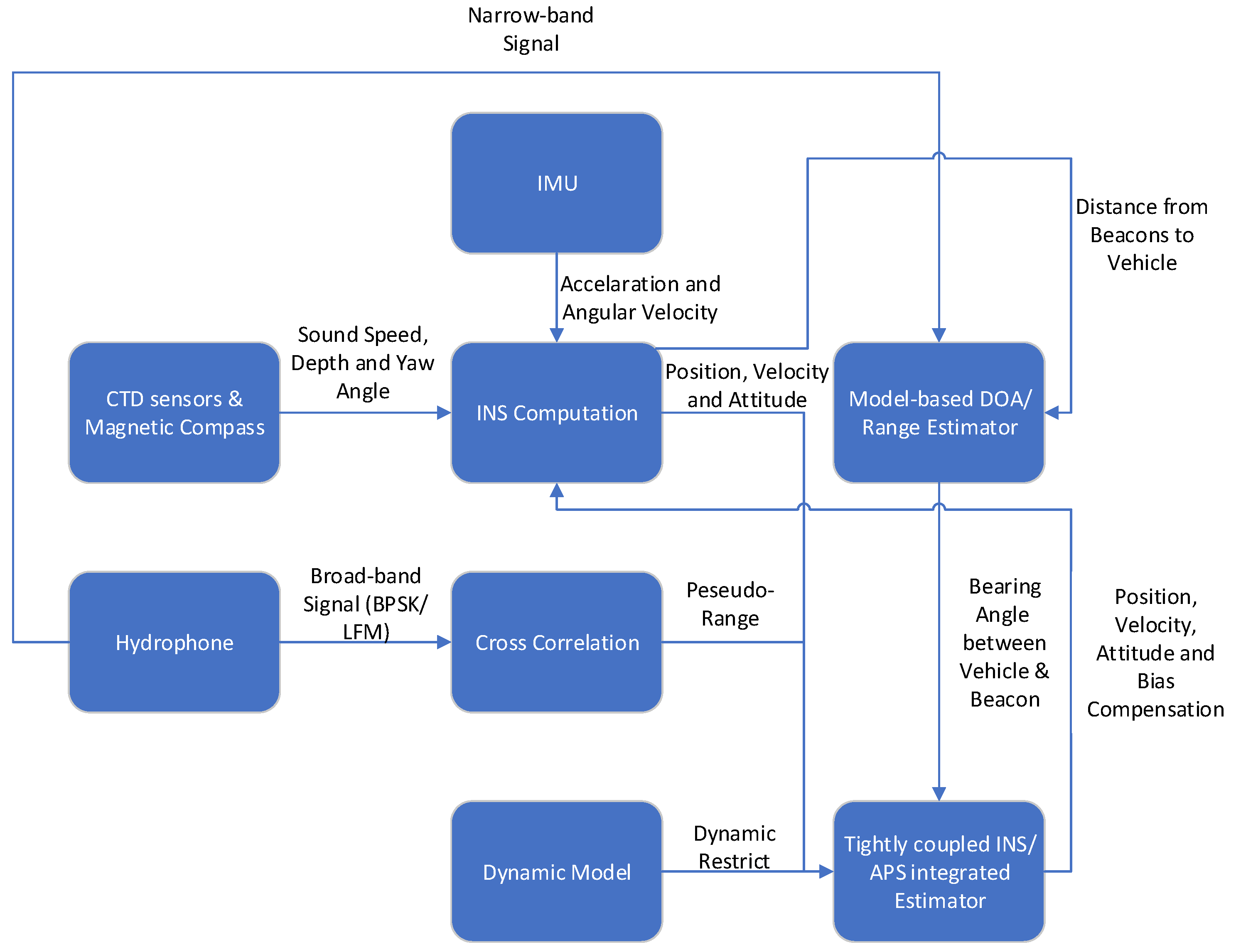
After reviewing several studies, Refs. [13,27] describe the detailed mathematical derivation of the state-space model based on the INS/acoustic beacon systems. In this paper, we establish the underwater integrated navigation model based on these studies. Four frames are used in this paper: body frame (subscript b denotes body frame), East-North-Up local-level frame (subscript n denotes body frame), Earth-Cantered Earth-Fixed Frame (subscript ECEF denotes this frame), Longitude-Latitude-Altitude frame (subscript LLA denotes this frame). Detailed information about these frames can be found in [28].

The overview block diagram of the integrated navigation system is displayed in Figure 1. Aiming to improve the accuracy of navigation in low-SNR conditions, we try to use any possible information that helps reduce the accumulating error of INS. Using the APS system, we can analyze the signal from beacons and obtain DOA and range information directly. The beacon transmits a narrow-band signal (single-frequency signal) and a modulated broadband signal in the meantime. The underwater vehicle equipped with a hydrophone array receives and processes the signal, and then obtains the bearing and distance information.

Furthermore, transforming temporal gain to spatial gain is also possible to increase the accuracy of acoustic DOA and range measurement. Inspired by the model-based signal processing methods for underwater array [10], we design a model-based estimator and realize the joint spatial synthetic DOA/range estimation.

The diagram in Figure 1 shows that the system can be divided into DOA/range estimation and tightly coupled navigation. The former estimates the bearing angle and distance between AUV and beacons. This process is aided by the navigation result. The latter uses the bearing and range information to correct the results of INS dead reckoning.

Two discrete-time state-space models are established. A detailed description of the models are discussed in Section 3. INS computation and cross-correlation algorithms are well-researched [28], which will not be discussed in this paper.

3. Methodology

In this section, mathematical modeling and derivation of the DOA/range estimator and the tightly coupled INS/APS integrated estimator are discussed. Both estimators are based on the unscented Kalman filter (UKF). In the discrete-time domain, the state-space model is as follows:

$$\begin{array}{cc}\hfill X_{k+1}& =F\left(X_k\right)+W_k\hfill \end{array}$$

(1)

$$\begin{array}{cc}\hfill Z_{k+1}& =H\left(X_{k+1}\right)+V_k\hfill \end{array}$$

(2)

where $X_k$, $Z_k$, $W_k$, and $V_k$ represent the state vector, the measurement vector, the system noise, and the measurement noise, respectively. Both $W_k$ and $V_k$ are viewed as zero-mean, Gaussian white noise. $F\left(\right)$ and $H\left(\right)$ represent the state transition function and measurement transition function, respectively. Although the model is not restricted to the single beacon situation, to simplify the problem, we only discuss the single beacon case in this section.

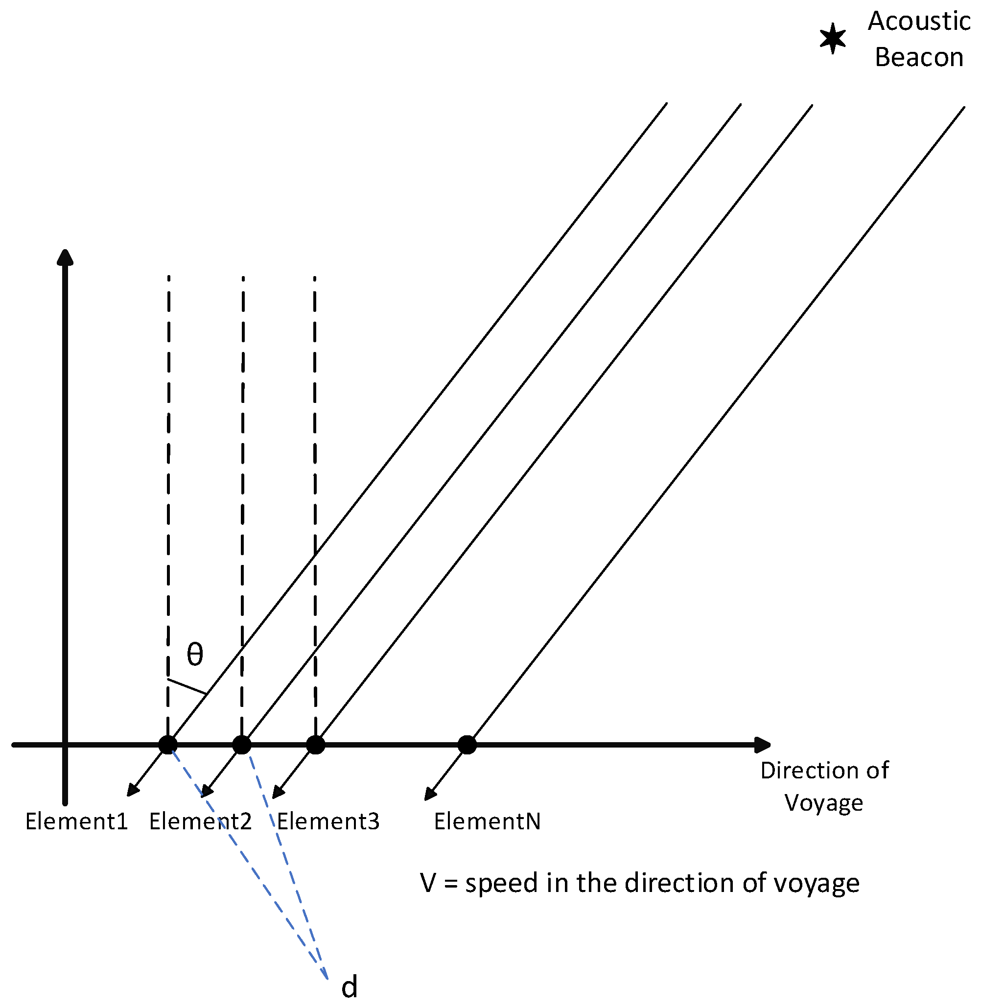
3.1. DOA/Range Estimator

One possible way to improve positioning accuracy in low-SNR conditions is transforming temporal gain into spatial gain. Based on the theory of Sullivan [10], we establish a DOA/range joint estimation model. Figure 2 shows the basic application scenario of the moving hydrophone array.

3.1.1. The System Model

The state vector is defined as follows:

$${\mathit{X}}_k={[{\theta }_k,b_k,R_k,V_k,{\omega }_k,{ϵ}_k,a_k]}^T$$

(3)

where ${\theta }_k$ represents the bearing angle; $b_k$ represents the bearing rate; $R_k$ represents the distance between the vehicle (can be viewed as the first hydrophone node) and the beacon; $V_k$ represents the velocity component in the voyage direction; ${\omega }_k$ is the frequency of the single-frequency signal; ${ϵ}_k$ is the frequency deviation due to environmental disturbance; $a_k$ is the amplitude of the single-frequency signal. The subscript k represents the kth epoch.

Based on Figure 2, the acoustic signal can be viewed as a plane wave. The dynamic model of the vehicle is assumed to be the mild-change constant-velocity model. So, in system estimation, the bearing rate $b_k$ and vehicle’s voyage velocity $V_k$ of the current epoch are equal to the values of the next epoch. We define T as the time interval of each epoch. Then, we can obtain ${\theta }_k={\theta }_{k-1}+b_{k-1}T$. According to cosine law (as Figure 3 shows), the recurrent equation between $R_k$ and $R_{k-1}$ can also be established. The frequency ${\omega }_k$ can be viewed as invariant in the system model. Therefore, the system state predicting equations of each component in $X_k$ are shown in (4). In this way, the recurrence relation between the state vectors in the current and the next epochs is built.

$$\left\{\begin{array}{c}{\theta }_k={\theta }_{k-1}+b_{k-1}T\hfill \\ b_k=b_{k-1}\hfill \\ R_k=\sqrt{R_{k-1}^2+{\left(V_{k-1}T\right)}^2-2R_{k-1}(V_{k-1}Tsin{\theta }_{k-1})}\hfill \\ V_k=V_{k-1}\hfill \\ {\omega }_k={\omega }_{k-1}\hfill \\ {ϵ}_k={ϵ}_{k-1}\hfill \\ a_k=a_{k-1}\hfill \end{array}\right.$$

(4)

In real applications, before the next epoch starts, the value of $V_k$ will be assigned to the velocity calculated by the navigation update.

3.1.2. The Measurement Model

The measurement vector $Z_k$ is defined as (5)~(7):

$$\begin{array}{cc}\hfill {\mathbf{Z}}_k& ={[{\mathbf{Pr}}_k,{\mathbf{Dis}}_k,\Delta {\omega }_k]}^T\hfill \end{array}$$

(5)

$$\begin{array}{cc}\hfill {\mathbf{Pr}}_k& =[P{r}_{k,1},P{r}_{k,2}\dots P{r}_{k,N}]\hfill \end{array}$$

(6)

$$\begin{array}{cc}\hfill {\mathbf{Dis}}_k& =[Di{s}_{k,1},Di{s}_{k,2}\dots Di{s}_{k,N}]\hfill \end{array}$$

(7)

$P{r}_{k,i}$ in (6) represents the received sound pressure of ith hydrophone element. The sound pressure describes the arriving sound signal. ${\mathbf{Pr}}_k$ represents the vector consisting of $P{r}_{k,i}$. $Di{s}_{k,i}$ in (7) represents the measured distance between the ith hydrophone element and the beacon. ${\mathbf{Pr}}_k$ is the vector consist of $P{r}_{k,i}$. $\Delta {\omega }_k$ represents the difference in frequency between the measured narrow-band signal and the ideal frequency of the original signal. Note that $P{r}_{k,i}$ is directly measured by the hydrophones; $Di{s}_{k,i}$ is indirectly obtained by calculating the distance between each hydrophone element and beacon position. $\Delta {\omega }_k$ is obtained from the frequency spectrum of a certain length of the signal sequence (a sliding temporal window).

According to Sullivan’s theory [10], the received sound pressure can be expressed by a function of ${\theta }_k$, $b_k$, $a_k$${\omega }_k$, and $V_k$. As more information can be provided by INS and OWTT, in this model, the received sound pressure $P{r}_{k,i}$ is a function of ${\theta }_k$, $b_k$, $a_k$, ${\omega }_k$, $V_k$, and ${ϵ}_k$. To avoid carrying the amplitude as a nuisance parameter, the phase of $P{r}_{k,i}$ is expressed by ${\theta }_k$, $b_k$, ${\omega }_k$, and ${ϵ}_k$ instead of using one parameter. The $Di{s}_{k,i}$ can be expressed as a function of $R_k$ and ${\theta }_k$ based on the shape of the array shown in Figure 2. According to the definition of $\Delta {\omega }_k$, $\Delta {\omega }_k$ contains two components: Doppler shift and environmental disturbance. In this way, $\Delta {\omega }_k$ can be expressed as a function of ${\theta }_k$, $V_k$, ${\omega }_k$, and ${ϵ}_k$. So, the predictive equations of measurement are shown in (8).

$$\left\{\begin{array}{c}P{r}_{k,i}=a_{k}cos[({\omega }_k+{ϵ}_k)t_k+{\beta }_i\left(t_k\right)sin{\theta }_k]\hfill \\ Di{s}_{k,i}=R_k-(i-1)dsin{\theta }_k\hfill \\ \Delta {\omega }_k=({\omega }_k+{ϵ}_k)(1+\frac{V_k}{c}sin{\theta }_k)-{\omega }_0\hfill \end{array}\right.$$

(8)

$${\beta }_i\left(t_k\right)=\frac{{\omega }_k}{c}[d(i-1)+V_k{t}_k]$$

(9)

In (8), $t_k$ represents the time point of the kth epoch. The definition of ${\beta }_i\left(t_k\right)$ is shown in (9). c represents the sound speed ${\omega }_0$ represents the ideal frequency of the narrow-band signal.

In this way, equations sets (4) and (8) can be written as two functions $F_D\left(X_k\right)$ and $H_D\left(X_k\right)$. So, the state model is finally written as (10).

$$\left\{\begin{array}{c}{\mathbf{X}}_{k+1}=F_D\left({\mathbf{X}}_k\right)+{\mathbf{W}}_k^D\hfill \\ {\mathbf{Z}}_k=H_D\left({\mathbf{X}}_k\right)+{\mathbf{V}}_k^D\hfill \\ {\mathbf{W}}_k^D\sim N(0,{\mathbf{Q}}_k)\hfill \\ {\mathbf{V}}_k^D\sim N(0,{\mathbf{R}}_k)\hfill \end{array}\right.$$

(10)

The resolution of the hydrophone array is approximately $0.886\frac{\lambda }{D}$, where $\lambda$ and D are the wavelengths of the signal and the aperture of the array. After iterations, the vehicle’s trajectory just synthesizes a long aperture of detection (although it is not formed at the same time). In this way, the temporal gain is transformed into spatial gain. The DOA estimation will be more accurate.

3.1.3. Observability Analysis

The observability of linear systems is well-researched while the observability of nonlinear systems is still a field of interest for many researchers. Based on the theorem established by these publications [29,30,31,32], one possible and convenient way to analyze the observability of the proposed model is linearizing the nonlinear system model and testing the observability matrix rank conditions.

The first-order linearized system model of the system (10) can be written as (11), which is a time-varying system. To be concise, we omit the noise terms in the model.

$$\left\{\begin{array}{c}{\mathbf{X}}_{k+1}=\frac{\partial F_D}{\partial \mathbf{X}}{|}_{{\mathbf{X}}_k}{\mathbf{X}}_k={\mathbf{A}}_{k|k+1}{\mathbf{X}}_k\hfill \\ {\mathbf{Z}}_k=\frac{\partial H_D}{\partial \mathbf{X}}{|}_{{\mathbf{X}}_k}{\mathbf{X}}_k={\mathbf{C}}_k{\mathbf{X}}_k\hfill \end{array}\right.$$

(11)

The detailed components of the matrices ${\mathbf{A}}_{k|k+1}$ and ${\mathbf{C}}_k$ is shown in (12)–(15). Unlike time-invariant systems, several different observability methods are defined for time-varying systems. They are complete observability, differential observability, instantaneous observability, and local observability [32,33,34]. In this paper, we analyze the local observability of the proposed model. In this way, we will know the restrictions when the model is available.

$${\mathbf{A}}_{k|k+1}=\left[\begin{array}{ccccccc}1& T& 0& 0& 0& 0& 0\\ 0& 1& 0& 0& 0& 0& 0\\ A_{3,1}& 0& A_{3,3}& A_{3,4}& 0& 0& 0\\ 0& 0& 0& 1& 0& 0& 0\\ 0& 0& 0& 0& 1& 0& 0\\ 0& 0& 0& 0& 0& 1& 0\\ 0& 0& 0& 0& 0& 0& 1\end{array}\right]$$

(12)

$$\left\{\begin{array}{cc}{A}_{3,1}=\hfill & -{[R_k^2+{\left(V_{k}T\right)}^2-2R_k(V_{k}Tsin{\theta }_k)]}^{-\frac{1}{2}}\hfill \\ \hfill & ·\left(R_k{V}_{k}T\right)cos{\theta }_k\hfill \\ A_{3,3}=\hfill & {[R_k^2+{\left(V_{k}T\right)}^2-2R_k(V_{k}Tsin{\theta }_k)]}^{-\frac{1}{2}}\hfill \\ \hfill & ·(R_k-V_{k}Tsin{\theta }_k)\hfill \\ A_{3,4}=\hfill & {[R_k^2+{\left(V_{k}T\right)}^2-2R_k(V_{k}Tsin{\theta }_k)]}^{-\frac{1}{2}}\hfill \\ \hfill & ·(T^2{V}_k-R_{k}Tsin{\theta }_k)\hfill \end{array}\right.$$

(13)

$${\mathbf{C}}_k=\left[\begin{array}{ccccccc}P{r}_{1,1}& 0& 0& P{r}_{1,4}& P{r}_{1,5}& P{r}_{1,6}& P{r}_{1,7}\\ P{r}_{2,1}& 0& 0& P{r}_{2,4}& P{r}_{2,5}& P{r}_{2,6}& P{r}_{2,7}\\ ⋮& ⋮& ⋮& ⋮& ⋮& ⋮& ⋮\\ P{r}_{N,1}& 0& 0& P{r}_{N,4}& P{r}_{N,5}& P{r}_{N,6}& P{r}_{N,7}\\ Di{s}_{1,1}& 0& 1& 0& 0& 0& 0\\ Di{s}_{2,1}& 0& 1& 0& 0& 0& 0\\ ⋮& ⋮& ⋮& ⋮& ⋮& ⋮& ⋮\\ Di{s}_{N,1}& 0& 1& 0& 0& 0& 0\\ \Delta {\omega }_{1,1}& 0& 0& \Delta {\omega }_{1,4}& \Delta {\omega }_{1,5}& \Delta {\omega }_{1,6}& 0\end{array}\right]$$

(14)

$$\left\{\begin{array}{c}P{r}_{i,1}=-a_k·{\beta }_i\left(t_k\right)·cos{\theta }_{k}sin[({\omega }_k+{ϵ}_k)t_k+{\beta }_i\left(t_k\right)sin{\theta }_k]\hfill \\ P{r}_{i,4}=-a_k\frac{{\omega }_k{t}_{k}sin{\theta }_k}{c}sin[({\omega }_k+{ϵ}_k)t_k+{\beta }_i\left(t_k\right)sin{\theta }_k]\hfill \\ \begin{array}{cc}P{r}_{i,5}=& -a_k(t_k+\frac{[d·(i-1)+V_k{t}_k]·sin{\theta }_k}{c})sin[({\omega }_k+{ϵ}_k)t_k\\ & +{\beta }_i\left(t_k\right)sin{\theta }_k]\hfill \end{array}\hfill \\ P{r}_{i,6}=-a_k{t}_k·sin[({\omega }_k+{ϵ}_k)t_k+{\beta }_i\left(t_k\right)sin{\theta }_k]\hfill \\ P{r}_{i,7}=cos[({\omega }_k+{ϵ}_k)t_k+{\beta }_i\left(t_k\right)sin{\theta }_k]\hfill \\ Di{s}_{i,1}=(1-i)·d·cos{\theta }_k\hfill \\ \Delta w_{i,1}=({\omega }_k+{ϵ}_k)·cos{\theta }_k\hfill \\ \Delta w_{i,4}=({\omega }_k+{ϵ}_k)·\frac{sin{\theta }_k}{c}\hfill \\ \Delta w_{i,5}=1+\frac{V_k}{c}sin{\theta }_k\hfill \\ \Delta w_{i,6}=1+\frac{V_k}{c}sin{\theta }_k\hfill \\ (i=1,2,3\dots N)\hfill \end{array}\right.$$

(15)

Definition 1

(Local Observability). Let n denote the dimension of the state vector $x_k$. A time-varying system is defined as:

$x_{k+1}=f_k\left(x_k\right)$

$y_k=h_k\left(x_k\right)$

If the state $x_k$ can be determined from $y_j$ where $j=k,k+1,\cdots ,k+n-1$, then the system is locally observable.

Then, the local observability matrix of System (11) on the kth iteration can be written as (16).

$$O_k=\left[\begin{array}{c}{\mathbf{C}}_k\\ {\mathbf{C}}_{k+1}{\mathbf{A}}_k\\ {\mathbf{C}}_{k+2}{\mathbf{A}}_{k+1}{\mathbf{A}}_k\\ ⋮\\ {\mathbf{C}}_{k+n-1}{\mathbf{A}}_{k+n-2}\dots {\mathbf{A}}_{k+1}{\mathbf{A}}_k\end{array}\right]$$

(16)

If the system is locally observable, the rank of $O_k$ should be of rank n, where $n=7$ in this case. After testing the local observability matrix of the (11), two interesting results are obtained:

• When there is only one element of the hydrophone “array”, $rank\left(O_k\right)=5$. So the system is unobservable if the hydrophone “array” only contains one element. This property is also proven by [10,35], but in a different way.
• The system (10) is undifferentiable if $R_k^2+{\left(V_{k}T\right)}^2-2R_k(V_{k}Tsin{\theta }_k)=0$. This will happen if and only if $\theta =\pm \frac{\pi }{2}$ and $R_k=\pm V_k·T$. Therefore, the model is unobservable if the trajectory of the AUV overlaps the position of the beacon. This result is also supported by the research of [9] but in a different aspect. Wang discussed the basic TOA/DOA single beacon localization geometric model and pointed out that the geometric state transformation matrix is not invertible when the vehicle’s trajectory overlaps the position of the beacon. However, unlike pure DOA or pure TOA localization method, when $\theta =\frac{\pi }{2}$ and $R_k\ne V_k·T$ (the trajectory of the vehicle is collinear with the beacon but does not overlap the beacon), the system is still observable.

3.1.4. UKF

One fact is that $F_D\left({\mathbf{X}}_k\right)$ and $H_D\left({\mathbf{X}}_k\right)$ are not linear function. The conventional Kalman filter is not a suitable choice when we consider the data-fusion problem. While using the extended Kalman filter to solve the problem, it is hard work to calculate the time-varying Jacobian matrix in every iteration. So, we finally choose the unscented Kalman filter (UKF). The mathematical principle of UKF is well researched [36], so this paper will not list the concrete derivation of UKF. The specific steps of UKF in this model are shown in

Table 2. The process of UKF in DOA/range estimation.

Set up parameters
$N_x$—the dimension of the state vector $X_k$	$\left\{\begin{array}{c}{G}_m^0=\frac{\lambda }{N_x+\lambda }\hfill \\ G_m^i=\frac{\lambda }{2(N_x+\lambda )}\hfill \\ G_m^{i+N_x}=\frac{\lambda }{2(N_x+\lambda )}\hfill \\ G_c^0=\frac{\lambda }{N_x+\lambda }+1+\beta -{\alpha }^2\hfill \\ G_c^i=\frac{\lambda }{2(N_x+\lambda )}\hfill \\ G_c^{i+N_x}=\frac{\lambda }{2(N_x+\lambda )}\hfill \\ i=1,2,3\dots N_x\hfill \end{array}\right.$
$N_y$—the dimension of the measurement vector $Z_k$
$\alpha$—a tuning parameter, commonly set to be ${10}^{-3}$
$\beta$—a tuning parameter, commonly set to be 2
$\kappa$—a tuning parameter, a heuristic rule commonly used is to set $N_x+\kappa =3$
$\lambda$—$\lambda ={\alpha }^2\times (N_x+\kappa )-N_x$
$G_m^i$—the weight value in state prediction
$G_c^i$—the weight value in state error covariance prediction
$Q_k$—the system noise covariance matrix
$R_k$—the measurement noise covariance matrix
$P_k$—-the state error covariance matrix
Generate sigma points
Define $Cholesky\left(\mathit{A}\right)$ as the Cholesky decomposition of $\mathit{A}$.	${\mathit{P}}_k=\mathit{U}{\mathit{A}}_k{\mathit{V}}^{\mathit{T}}$—(SVD)
	${\mathit{S}}_k=\mathit{U}·Cholesky\left({\mathit{A}}_k\right)$
Define ${\left(\mathit{A}\right)}_i$ as the ith column of matrix $\mathit{A}$. The total number of the sigma points is $2N_x+1$.	$\left\{\begin{array}{c}{\mathit{X}}_k^0={\mathit{X}}_k\hfill \\ {\mathit{X}}_k^i={\mathit{X}}_k+{\left(\sqrt{N_x+\lambda }{\mathit{S}}_k\right)}_i\hfill \\ {\mathit{X}}_k^i={\mathit{X}}_k-{\left(\sqrt{N_x+\lambda }{\mathit{S}}_k\right)}_i\hfill \end{array}\right.$
	$i=1,2,3\dots N_x$
State prediction
Calculate the results after state transformation of all sigma points, and then calculate the weighted summation.	${\mathit{X}}_{k|k+1}^i=F_D\left({\mathit{X}}_k^i\right)$
	$i=0,1,2,3\dots 2N_x$
	${\mathit{X}}_{k|k+1}={\sum }_{i=0}^{2N_x}{G}_m^i{\mathit{X}}_{k|k+1}^i$
State error covariance prediction
Predict the state error covariance matrix.	${\tilde{\mathit{X}}}_{k|k+1}^i={\mathit{X}}_{k|k+1}^i-X_{k|k+1}$
	$i=0,1,2,3\dots 2N_x$
	${\mathit{P}}_{k|k+1}={\sum }_{i=0}^{2N_x}{G}_c^i{\tilde{\mathit{X}}}_{k|k+1}^i·{\left({\tilde{\mathit{X}}}_{k|k+1}^i\right)}^T+{\mathit{Q}}_k$
Update sigma points
Generate the new sigma points after state prediction.	${\mathit{P}}_{k|k+1}=\mathit{U}{\mathit{A}}_{k|k+1}{\mathit{V}}^{\mathit{T}}$—(SVD)
	${\mathit{S}}_{k|k+1}=\mathit{U}·Cholesky\left({\mathit{A}}_{k|k+1}\right)$
	$\left\{\begin{array}{c}{\mathit{Y}}_{k|k+1}^0={\mathit{X}}_{k|k+1}\hfill \\ {\mathit{Y}}_{k|k+1}^i={\mathit{X}}_{k|k+1}+{\left(\sqrt{N_x+\lambda }{\mathit{S}}_{k|k+1}\right)}_i\hfill \\ {\mathit{Y}}_{k|k+1}^i={\mathit{X}}_{k|k+1}-{\left(\sqrt{N_x+\lambda }{\mathit{S}}_{k|k+1}\right)}_i\hfill \end{array}\right.$
	$i=1,2,3\dots N_x$
Measurement prediction
Predict the measurement vector by state vector.	${\mathit{Z}}_{k|k+1}^i=H_D\left({\mathit{Y}}_{k|k+1}^i\right),i=1,2,3\dots 2N_x$
	${\mathit{Z}}_{k|k+1}={\sum }_{i=0}^{2N_x}{G}_m^i{\mathit{Z}}_{k|k+1}^i$
	${\tilde{\mathit{Z}}}_{k|k+1}^i={\mathit{Z}}_{k|k+1}^i-Z_{k|k+1}$
	${\mathit{P}}_{k|k+1}^z={\sum }_{i=0}^{2N_x}{G}_c^i{\tilde{\mathit{Z}}}_{k|k+1}^i·{\left({\tilde{\mathit{Z}}}_{k|k+1}^i\right)}^T+{\mathit{R}}_k$
	${\mathit{P}}_{k|k+1}^{xz}={\sum }_{i=0}^{2N_x}{G}_c^i{\tilde{\mathit{X}}}_{k|k+1}^i·{\left({\tilde{\mathit{Z}}}_{k|k+1}^i\right)}^T+{\mathit{R}}_k$
State update
Update the state by introduce real measurement.	${\mathit{K}}_{k+1}=P_{k|k+1}^{xz}{\left(P_{k|k+1}^z\right)}^{-1}$
	${\widehat{\mathit{X}}}_{k+1}={\mathit{X}}_{k|k+1}+{\mathit{K}}_{k+1}({\mathit{Z}}_{k+1}-{\mathit{Z}}_{k|k+1})$
	${\mathit{P}}_{k+1}={\mathit{P}}_{k|k+1}-{\mathit{K}}_{k+1}{\mathit{P}}_{k|k+1}^z{\mathit{K}}_{k+1}^T$

.

Because of the floating-point error in real computation, when the elements of ${\mathbf{P}}_k$ are small, ${\mathbf{P}}_k$ will sometimes become negative definite using the standard UKF algorithm. There is no solution for Cholesky decomposition in this case. To guarantee the positive semidefiniteness of ${\mathbf{S}}_k$, unlike the standard UKF algorithm, we add a singular value decomposition (SVD) step before Cholesky decomposition, which is shown in the “Generate sigma points” step of Table 2.

The covariance matrix ${\mathbf{P}}_k$ can always be decomposed as (17):

$${\mathbf{P}}_k=\mathbf{U}{\mathbf{A}}_k\mathbf{V}$$

(17)

Based on the definition of SVD, ${\mathbf{A}}_k$ always meets the condition of positive semidefinite. Because the covariance matrix is symmetric. Then we can obtain:

$$\begin{array}{cc}\hfill & {\mathbf{P}}_k=\mathbf{U}\sqrt{{\mathbf{A}}_k{\mathbf{A}}_k^T}{\mathbf{U}}^T\hfill \end{array}$$

(18)

$$\begin{array}{cc}\hfill & Cholesky\left({\mathbf{P}}_k\right)=\mathbf{U}·Cholesky\left({\mathbf{A}}_k\right)\hfill \end{array}$$

(19)

This method prevents the anomaly of Cholesky decomposition over iterations which is also used in the filter of the tightly coupled INS/APS navigation Estimator.

3.2. Tightly Coupled INS/APS Navigation Estimator

For underwater vehicles’ navigation, yaw angle and depth are instrumented adequately with the compass and the depth gauge. So, long-range underwater navigation can be viewed as a 2D problem. Traditional single beacon integrated navigation algorithms should calculate the position of the vehicle, and then the position error model is used for data-fusion. This strategy has disadvantages, such as motion restriction and multi-results. So, in the proposed model, inspired by the tightly coupled INS/GNSS navigation, the tightly coupled strategy is chosen for INS/APS navigation. Kepper proposes an open-loop architecture for 2D underwater integrated navigation [37]. However, it has been proven in INS/GNSS integrated navigation that the closed-loop architecture is more stable and has better performance in practice [38]. The closed-loop architecture is then used in the proposed model.

3.2.1. The System Model

The state vector is defined as follows:

$$\begin{array}{c}\hfill {\mathbf{Xn}}_k=[\delta P_{E,k},\delta P_{N,k},\delta V_{E,k},\delta V_{N,k},\delta {\varphi }_k,\delta {\theta }_k,\\ \hfill \delta {\gamma }_k,\delta b_{x,k},\delta b_{y,k},\delta b_{z,k},\delta g_{x,k},\delta g_{y,k},\delta g_{z,k},\delta cl{k}_k{]}^T\end{array}$$

(20)

$\delta P_{E,k},\delta P_{N,k}$ represent the error in Longitude and Latitude respectively; $\delta V_{E,k}$ and $\delta V_{N,k}$ represent the error of eastward velocity and northward velocity respectively; ${\varphi }_k,\delta {\theta }_k$, and $\delta {\gamma }_k$ represent the error of the pitch, roll, and yaw angle, respectively; $\delta b_{x,k},\delta b_{y,k}$, and $\delta b_{z,k}$ are the error of 3-axis accelerometers’ bias in body frame; $\delta g_{x,k},\delta g_{y,k}$, and $\delta g_{z,k}$ are the error of 3-axis gyroscopes’ bias in body frame; $\delta cl{k}_k$ is the drift of OWTT caused by clock defects or propagation channel.

Because the changing process of bias and drift are modeled with first-order Gauss–Markov process [13], the bias can be written in the form of (21), where $Tc$ is the correlation time, $dt$ is the sample period of the filter and $w_b$ is the zero mean Gaussian noise of bias.

$$b_k=e^{\frac{dt}{T_c}}{b}_{k-1}+w_b$$

(21)

Based on the classic inertial error model [28], the state transition model can be finally written as (22) to (27).

$$\left[\begin{array}{c}\delta P_{E,k+1}\\ \delta P_{N,k+1}\end{array}\right]=\left[\begin{array}{cc}0& \frac{dt}{R_M+h}\\ \frac{dt}{(R_N+h)cos\left(Lon\right)}& 0\end{array}\right]\left[\begin{array}{c}\delta V_{E,k}\\ \delta V_{N,k}\end{array}\right]+\left[\begin{array}{c}\delta P_{E,k}\\ \delta P_{N,k}\end{array}\right]$$

(22)

$$\left[\begin{array}{c}\delta V_{E,k+1}\\ \delta V_{N,k+1}\end{array}\right]=\left[\begin{array}{c}\delta V_{E,k}\\ \delta V_{N,k}\end{array}\right]+C_b^n(1:2,1:3)\left[\begin{array}{c}\delta b_{x,k}\\ \delta b_{y,k}\\ \delta b_{z,k}\end{array}\right]$$

(23)

$$\begin{gathered} \left[\begin{array}{c}\delta {\varphi }_{k+1}\\ \delta {\theta }_{k+1}\\ \delta {\gamma }_{k+1}\end{array}\right]=\left[\begin{array}{c}\delta {\varphi }_k\\ \delta {\theta }_k\\ \delta {\gamma }_k\end{array}\right]+C_b^n\left[\begin{array}{c}\delta g_{x,k}\\ \delta g_{y,k}\\ \delta g_{z,k}\end{array}\right]dt \\ +\left[\begin{array}{cc}0& \frac{dt}{R_M+h}\\ \frac{-dt}{R_N+h}& 0\\ \frac{-dttan\left(lon\right)}{R_N+h}& 0\end{array}\right]\left[\begin{array}{c}\delta V_{E,k}\\ \delta V_{N,k}\end{array}\right] \end{gathered}$$

(24)

$$\left[\begin{array}{c}\delta b_{x,k+1}\\ \delta b_{y,k+1}\\ \delta b_{z,k+1}\end{array}\right]=e^{-\frac{dt}{T{c}_1}}\left[\begin{array}{c}\delta b_{x,k}\\ \delta b_{y,k}\\ \delta b_{z,k}\end{array}\right]$$

(25)

$$\left[\begin{array}{c}\delta g_{x,k+1}\\ \delta g_{y,k+1}\\ \delta g_{z,k+1}\end{array}\right]=e^{-\frac{dt}{T{c}_2}}\left[\begin{array}{c}\delta g_{x,k}\\ \delta g_{y,k}\\ \delta g_{z,k}\end{array}\right]$$

(26)

$$\begin{array}{cc}\hfill \delta cl{k}_{k+1}& =e^{-\frac{dt}{T{c}_3}}·\delta cl{k}_k\hfill \end{array}$$

(27)

$R_N$ represents the local normal radius; $R_M$ represents the local meridian radius; $C_b^n$ is the 3 × 3 rotation matrix from body frame to ENU frame; $dt$ is the updating period of navigation. $T{c}_1,T{c}_2,T{c}_3$ are introduced, which are the correlation time constants of accelerators, gyroscopes, and clock, respectively.

3.2.2. The Measurement Model

The measurement vector is defined as (22) to (24).

$${\mathbf{Zn}}_k={[\delta {\rho }_k,\delta sin{\theta }_k]}^T$$

(28)

$$\delta {\rho }_k={\rho }_k^{INS}-{\rho }_k^{APS}$$

(29)

$$\delta sin{\theta }_k=\delta sin{\theta }_k^{INS}-\delta sin{\theta }_k^{APS}$$

(30)

$\delta {\rho }_k$ represents the difference between the distance measured by OWTT range and calculated by the navigation results of the last iteration; $\delta sin{\theta }_k$ represents the differences between the bearing angle measured by DOA and calculated by the navigation results of the last iteration.

The measurement vector can be predicted by state vector as equations in (31) to (36) show.

$${\mathbf{P}}_{ECEF}^{EST}=\left[\begin{array}{c}{x}_k\\ y_k\\ z_k\end{array}\right]=C_{LLA}^{ECEF}\left[\begin{array}{c}{P}_{E,k}-\delta P_{E,k}\\ P_{N,k}-\delta P_{N,k}\\ P_{U,k}\end{array}\right]$$

(31)

$$\begin{array}{cc}\hfill {\mathbf{P}}_{ECEF}^{beacon}& ={\left[\begin{array}{c}x{1}_k\\ y{1}_k\\ z{1}_k\end{array}\right]}_{ECEF}\hfill \end{array}$$

(32)

$$\begin{array}{cc}\hfill {\mathbf{P}}_{LLA}^{beacon}& ={\left[\begin{array}{c}{P}_E^{beacon}\\ P_N^{beacon}\\ P_U^{beacon}\end{array}\right]}_{LLA}\hfill \end{array}$$

(33)

$$\begin{array}{cc}\hfill {\mathbf{P}}_{ECEF}^{INS}& =C_{LLA}^{ECEF}\left[\begin{array}{c}{P}_{E,k}\\ P_{N,k}\\ P_{U,k}\end{array}\right]\hfill \end{array}$$

(34)

$$\begin{array}{cc}\hfill \delta \rho =& ∥{\mathbf{P}}_{ECEF}^{INS}-{\mathbf{P}}_{ECEF}^{beacon}∥-∥{\mathbf{P}}_{ECEF}^{EST}-{\mathbf{P}}_{ECEF}^{beacon}∥\hfill \\ & -c·\delta clk\left(k\right)\hfill \end{array}$$

(35)

$$\begin{array}{c}\hfill \delta sin{\theta }_k=sin\left[bearing((P_{E,k},P_{N,k}),(P_m^E,P_m^N))\right]-\\ \hfill sin\left[bearing((P_{E,k}-\delta P_{E,k},P_{N,k}-\delta P_{N,k}),(P_m^E,P_m^N))\right]\end{array}$$

(36)

$C_{LLA}^{ECEF}$ is 3 × 3 rotation matrix from LLA frame to ENU frame; ${\mathbf{P}}_{ECEF}^{beacon}$ is the beacon’s position in ECEF frame; ${\mathbf{P}}_{LLA}^{beacon}$ is the beacon’s position in LLA frame; $bearing(A,B)$ represents the bearing of point B from point A.

By combining the transformation equations, the state model of the tightly coupled model can be written in a concise form as (37).

$$\left\{\begin{array}{c}{\mathbf{Xn}}_{k+1}=F_{TC}\left({\mathbf{Xn}}_k\right)+{\mathbf{W}}_k^{TC}\hfill \\ {\mathbf{Zn}}_{k+1}=H_{TC}\left({\mathbf{Xn}}_{k+1}\right)+{\mathbf{V}}_{k+1}^{TC}\hfill \\ {\mathbf{W}}_k^{TC}\sim N(0,{\mathbf{Qn}}_k)\hfill \\ {\mathbf{V}}_k^{TC}\sim N(0,{\mathbf{Rn}}_k)\hfill \end{array}\right.$$

(37)

Note that the model can be transformed into the multi-beacon form by extending the measurement vector and transform function; similar to what (38) to (41) show, where m is the number of beacons. The only difference between each $H_{TC}^i\left(\right)$ is the position of the $i_{th}$ beacon.

$$\begin{array}{cc}\hfill {\mathit{Zn}}_k& ={[{\mathbf{\delta }\mathbf{\rho }}_k,{\mathbf{\delta }\mathit{bear}}_k]}^T\hfill \end{array}$$

(38)

$$\begin{array}{cc}\hfill {\mathbf{\delta }\mathbf{\rho }}_k& =[\delta {\rho }_k^1,\delta {\rho }_k^2,\delta {\rho }_k^3\dots \delta {\rho }_k^m]\hfill \end{array}$$

(39)

$$\begin{array}{cc}\hfill {\mathbf{\delta }\mathit{bear}}_k& =[\delta sin{\theta }_k^1,\delta sin{\theta }_k^2,\delta sin{\theta }_k^3\dots \delta sin{\theta }_k^m]\hfill \end{array}$$

(40)

$$\begin{array}{cc}\hfill {\mathit{Zn}}_{k+1}& =\left[\begin{array}{c}{H}_{TC}^1\left({\mathit{Xn}}_{k+1}\right)\\ H_{TC}^2\left({\mathit{Xn}}_{k+1}\right)\\ H_{TC}^3\left({\mathit{Xn}}_{k+1}\right)\\ ⋮\\ H_{TC}^m\left({\mathit{Xn}}_{k+1}\right)\end{array}\right]+{\mathit{W}}_{k+1}^{multi-TC}\hfill \end{array}$$

(41)

The observability of the tightly coupled model is not discussed in this paper because it is a well-researched topic in INS/GNSS tightly coupled navigation area. Some of the analyses can be found in [28,39,40].

3.2.3. UKF

UKF is also used to realize the data fusion procedure of the tightly coupled nonlinear state model. The whole streamline is shown in

Table 3. The process of UKF in tightly coupled navigation.

Set up parameters
$N_{x1}$—the dimension of the state vector ${\mathit{Xn}}_k$	$\left\{\begin{array}{c}{G}_m^0=\frac{\lambda }{N_{x1}+\lambda }\hfill \\ G_m^i=\frac{\lambda }{2(N_{x1}+\lambda )}\hfill \\ G_m^{i+N_x}=\frac{\lambda }{2(N_{x1}+\lambda )}\hfill \\ G_c^0=\frac{\lambda }{N_{x1}+\lambda }+1+\beta -{\alpha }^2\hfill \\ G_c^i=\frac{\lambda }{2(N_{x1}+\lambda )}\hfill \\ G_c^{i+N_x}=\frac{\lambda }{2(N_{x1}+\lambda )}\hfill \\ i=1,2,3\dots N_{x1}\hfill \end{array}\right.$
$N_{y}1$—the dimension of the measurement vector ${\mathit{Zn}}_k$
$\alpha ,\beta ,\kappa ,\lambda ,G_m^i,G_c^i,$—the definition of these parameters are the same as in Table 2
${\mathit{Qn}}_k$—the system noise covariance matrix
${\mathit{Rn}}_k$—the measurement noise covariance matrix
${\mathit{Pn}}_k$—the state error covariance matrix
Generate sigma points
	${\mathit{Pn}}_k=\mathit{U}{\mathit{An}}_k{\mathit{V}}^{\mathit{T}}$—(SVD)
	${\mathit{Sn}}_k=\mathit{U}·Cholesky\left({\mathit{An}}_k\right)$
	$\left\{\begin{array}{c}{\mathit{Xn}}_k^0={\mathit{Xn}}_k\hfill \\ {\mathit{Xn}}_k^i={\mathit{Xn}}_k+{\left(\sqrt{N_{x1}+\lambda }{\mathit{Sn}}_k\right)}_i\hfill \\ {\mathit{Xn}}_k^i={\mathit{Xn}}_k-{\left(\sqrt{N_{x1}+\lambda }{\mathit{Sn}}_k\right)}_i\hfill \end{array}\right.$
	$i=1,2,3\dots 2N_{x1}$
State prediction
	${\mathit{Xn}}_{k|k+1}^i=F_{TC}\left({\mathit{Xn}}_k^i\right),i=0,1,2,3\dots 2N_{x1}$
	${\mathit{Xn}}_{k|k+1}={\sum }_{i=0}^{2N_x}{G}_m^i{\mathit{Xn}}_{k|k+1}^i$
State error covariance prediction
	${\widetilde{\mathit{Xn}}}_{k|k+1}^i={\mathit{Xn}}_{k|k+1}^i-{Xn}_{k|k+1}$
	$i=0,1,2,3\dots 2N_{x1}$
	${\mathit{Pn}}_{k|k+1}={\sum }_{i=0}^{2N_{x1}}{G}_c^i{\widetilde{\mathit{Xn}}}_{k|k+1}^i·{\left({\widetilde{\mathit{Xn}}}_{k|k+1}^i\right)}^T+{\mathit{Qn}}_k$
Update sigma points
	${\mathit{Pn}}_{k|k+1}=\mathit{U}{\mathit{An}}_{k|k+1}{\mathit{V}}^{\mathit{T}}$—(SVD)
	${\mathit{Sn}}_{k|k+1}=\mathit{U}·Cholesky\left({\mathit{An}}_{k|k+1}\right)$
	$\left\{\begin{array}{c}{\mathit{Yn}}_{k|k+1}^0={\mathit{Xn}}_{k|k+1}\hfill \\ {\mathit{Yn}}_{k|k+1}^i={\mathit{Xn}}_{k|k+1}+{\left(\sqrt{N_{x1}+\lambda }{\mathit{Sn}}_{k|k+1}\right)}_i\hfill \\ {\mathit{Yn}}_{k|k+1}^i={\mathit{Xn}}_{k|k+1}-{\left(\sqrt{N_{x1}+\lambda }{\mathit{Sn}}_{k|k+1}\right)}_i\hfill \end{array}\right.$
	$i=1,2,3\dots N_{x1}$
Measurement prediction
	${\mathit{Zn}}_{k|k+1}^i=H_{TC}\left({\mathit{Y}}_{k|k+1}^i\right),i=1,2,3\dots 2N_{x1}$
	${\mathit{Zn}}_{k|k+1}={\sum }_{i=0}^{2N_x}{G}_m^i{\mathit{Zn}}_{k|k+1}^i$
	${\widetilde{\mathit{Zn}}}_{k|k+1}^i={\mathit{Zn}}_{k|k+1}^i-{Zn}_{k|k+1}$
	${\mathit{Pn}}_{k|k+1}^z={\sum }_{i=0}^{2N_{x1}}{G}_c^i{\widetilde{\mathit{Zn}}}_{k|k+1}^i·{\left({\widetilde{\mathit{Zn}}}_{k|k+1}^i\right)}^T+{\mathit{Rn}}_k$
	${\mathit{Pn}}_{k|k+1}^{xz}={\sum }_{i=0}^{2N_x}{G}_c^i{\widetilde{\mathit{Xn}}}_{k|k+1}^i·{\left({\widetilde{\mathit{Zn}}}_{k|k+1}^i\right)}^T+{\mathit{Rn}}_k$
State update
Update the state by introducing the real measurement, note that the updating step of ${\widehat{\mathit{Xn}}}_{k+1}$ is different.	${\mathit{Kn}}_{k+1}={\mathit{Pn}}_{k|k+1}^{xz}{\left({\mathit{Pn}}_{k|k+1}^z\right)}^{-1}$
	${\widehat{\mathit{Xn}}}_{k+1}={\mathit{Xn}}_{k|k+1}+{\mathit{Kn}}_{k+1}{\mathit{Zn}}_{k+1}$
	${\mathit{Pn}}_{k+1}={\mathit{Pn}}_{k|k+1}-{\mathit{Kn}}_{k+1}{\mathit{Pn}}_{k|k+1}^z{\mathit{Kn}}_{k+1}^T$

.

According to Section 3.1 and Section 3.2, it is possible if we combine two estimators into one by merging the state vectors and reorganizing the state-space model. However, the proposed model has lower computational consumption compared to the combined estimator with higher order. We quantified the computational complexity of every step in UKF, as shown in

Table 4. The computational complexity of UKF.

Step	Computational Complexity (N Is the Dimension of State Vector, L Is the Dimension of Measurement Vector)
Flops in State Prediction	$\frac{13}{3}{N}^3+11N^2+\frac{14}{3}N$
Flops in Measurement Update	$\frac{8}{3}{L}^3+12N{L}^2+2N^{2}L+\frac{15}{2}{L}^2+34NL+4N^2$ $+\frac{157}{6}L+N+3$
Flops in SVD	$\frac{8}{3}{N}^3$
Square Roots in Cholesky decomposition	N

. It is evident that the combined estimator will always require at least 56,593 more floating-point operations (flops) than the proposed model each filtering iteration.

On the other hand, the robustness of UKF will decrease if the dimension is too high. The results of the high-dimension filter will be hard to converge in some cases. Furthermore, it is difficult to select the best value of tuning parameters for high-dimension UKF. In consideration of these aspects, we choose the two estimators’ architectures in the proposed algorithm.

3.3. Parameters’ Selection and Motion Restriction

3.3.1. Parameters’ Selection

The system noise covariance matrix Q and the measurement covariance matrix R are the most important parameters for estimation for both estimators. It is hard to summarize a quantified rule of parameter selection. To say the least, however, we can obtain a qualitative rule. For DOA/range estimator, the selection of Q is based on the user’s trust in the constant-velocity dynamic model. R can be obtained from the noise of the navigation results and the measurement noise of sound pressure. For the tightly coupled navigation estimator, the selection of Q is based on the measurement noise of IMU and clock source. R’s selection is influenced by the measurement noise of OWTT and the estimation covariance of DOA. Most of the time, the value of Q should not be set too large, or the filter would be hard to converge. The value of R should be slightly larger than the measurement noise, which will help stabilize the filter’s results.

3.3.2. The Motion Restriction

There is no motion restriction for the tightly coupled navigation estimator, and it has already been proven observable all time [28]. However, for DOA/range estimator, because the basic assumption of the system model is constant velocity, the vehicle should move with a relatively stable velocity during estimation or the result of DOA/range estimation will deteriorate.

On the other hand, most of the single beacon navigation algorithms require the vehicle not to move radially towards or away from the beacon or the system will be unobservable. It has been proven in Section 3.1.3 that the proposed DOA/range estimator is also observable in the radial motion case if the trajectory does not overlap the position of beacons. In addition, there should be more than one element in the hydrophone array. The numeric analysis is presented in Section 4.1.

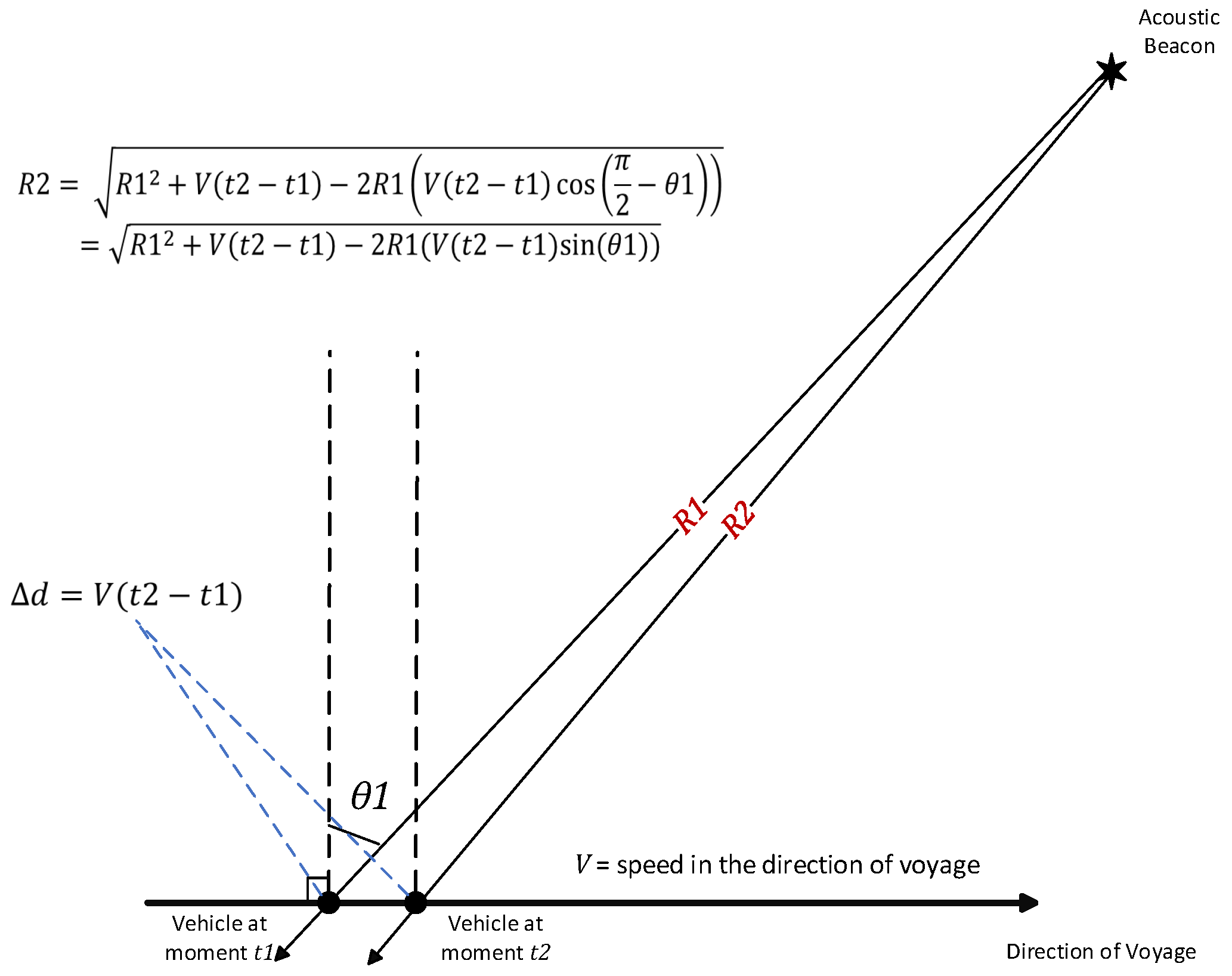
3.4. The OWTT Measurement

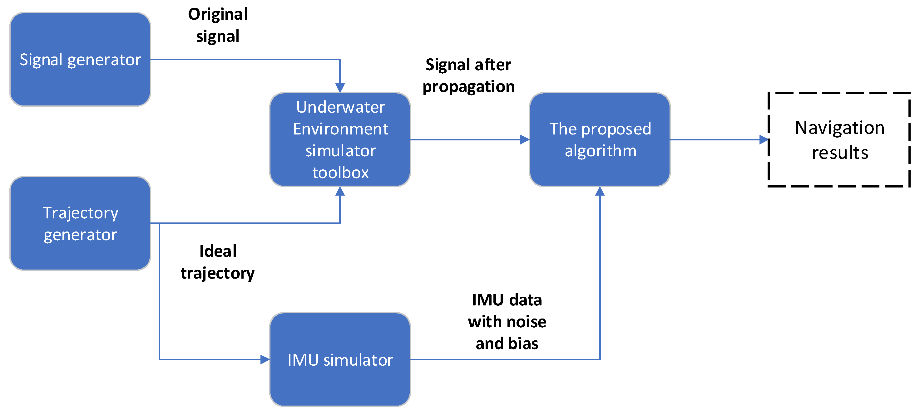
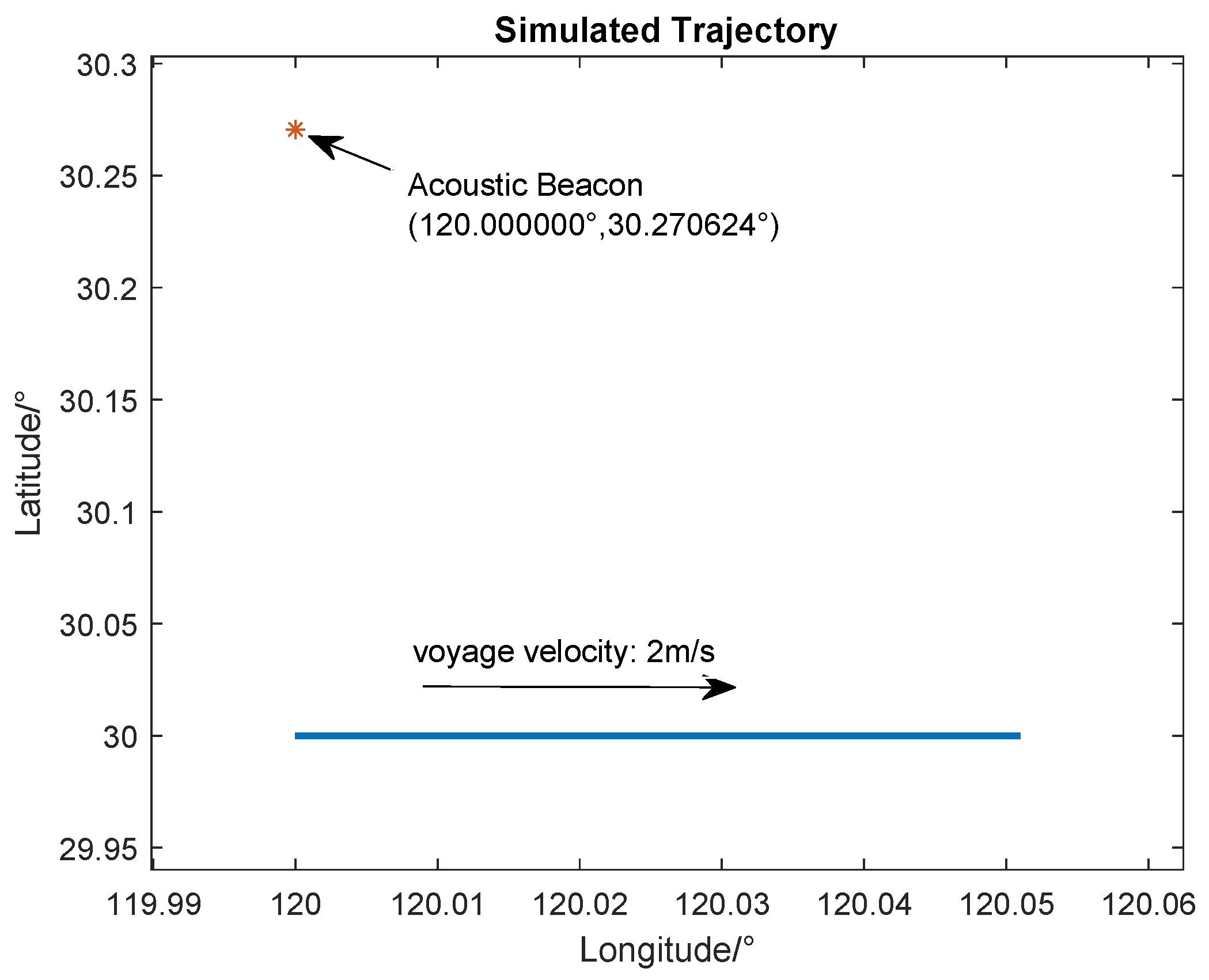
According to [1,3,13] and our experiments in East China Sea in 2021 (ECS2021), measuring the TOA of long-range through long-period modulated signal in shallow water is possible.

Figure 4 shows the error distribution of OWTT range measurement in the real stable experiment in ECS2021 (the acoustic transceiver and the hydrophones array are stable). The acoustic transceiver sent m-sequence data modulated by BPSK. The source level is about 170 dB re micro-pascal and the carrier frequency of the signal is 160 Hz with 16 Hz bandwidth. The correlation period is 30 s. The distance between the two ends is about 50 km. The result shows that the standard deviation of range measurement is about 8.5 m at 50 km. However, the error distribution shows that the noise is not zero-mean Gaussian noise, so we add a noise estimation variable $\delta cl{k}_k$ in the state vector of the tightly coupled navigation model.

The pseudo-code of the proposed algorithm is shown in Algorithm A1 (list in Appendix A).

4. Simulation

To verify the proposed method, we design a series of simulations including motion restriction and comparison of the proposed method with the pure inertial update and some recently proposed single-beacon algorithms in the same condition. The simulations were carried out in MATLAB. The block graph of the simulation system is shown in Figure 5.

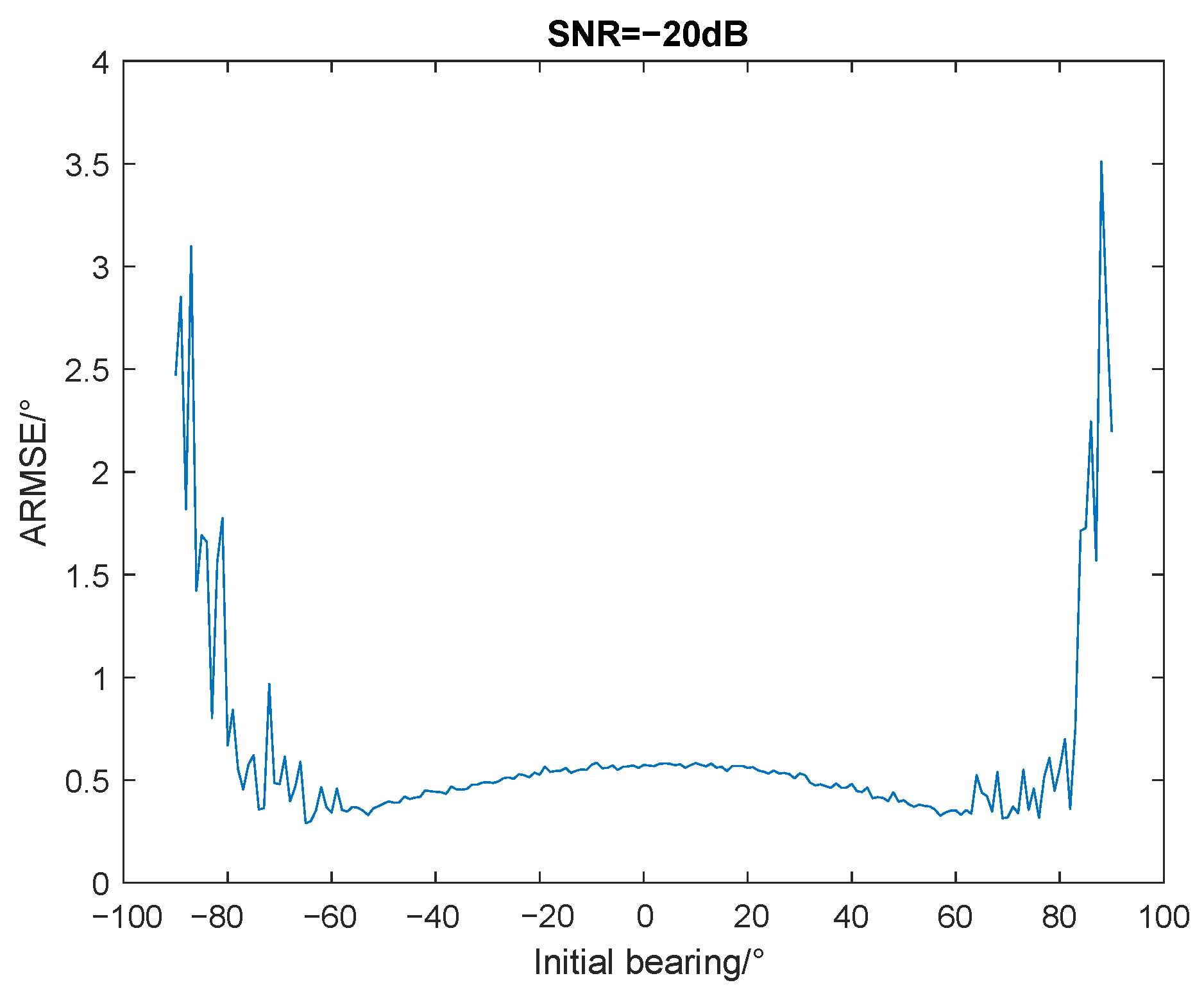
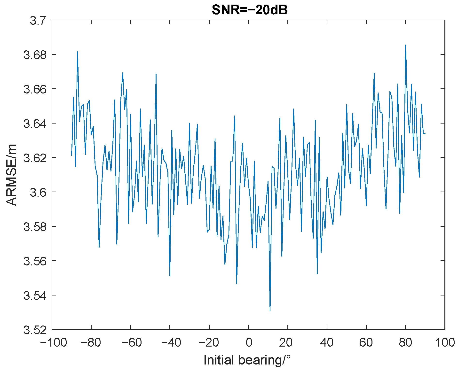
4.1. Motion Restriction Research

In this section, we use the numeric method to research the motion restriction of DOA/range estimator. To obtain the variation in accuracy of DOA/range estimator when the initial bearing is different, we set different start points of the vehicle in simulation. Except for bearing, the other parameters including heading direction, velocity and UKF parameters are all the same. The detailed configuration is shown in

Table 5. Simulation configuration in motion restriction research.

Parameter	Value
Number of hydrophone elements	10
Spatial interval of elements	5 m
Sample rate of hydrophone	4000 Hz
Sample rate of IMU	100 Hz
Time of simulation of each iteration	450 s
Times of repetition	50
Initial distance between the beacon and the vehicle	50 km
Voyage direction	East (yaw = 90${}^{\circ }$)
Voyage speed	2 m/s
Accuracy of depth sensor	0.1 m
Accuracy of Compass	0.1${}^{\circ }$
SNR	−20 dB
Frequency of narrowband signal	100 Hz
Broadband signal (a period)	LFM ($130\sim 230$ Hz, 40 s)
${\mathbf{Q}}_k$	$Diagonal({10}^{-7},{10}^{-8},{10}^{-6},{10}^{-9},{10}^{-4},{10}^{-5},{10}^{-6})$
${\mathbf{R}}_k$	$I_{21\times 21}\times {10}^{-3}$
${\mathbf{P}}_0$	$Diagonal(0.1,0.01,0.01,0.01,0.01,0.01,{10}^{-8})$
${\mathbf{Qn}}_k$	$Diagonal({10}^{-10},{10}^{-10},{10}^{-8},{10}^{-8},{10}^{-10},{10}^{-10},{10}^{-10},$ ${10}^{-12},{10}^{-12},{10}^{-12},{10}^{-12},{10}^{-12},{10}^{-12},{10}^{-12})$
${\mathbf{Rn}}_k$	$Diagonal({10}^4,{10}^4)$
${\mathbf{Pn}}_0$	$Diagonal({10}^{-8},{10}^{-8},{10}^{-6},{10}^{-6},{10}^{-8},{10}^{-8},{10}^{-10},$ ${10}^{-8},{10}^{-8},{10}^{-8},{10}^{-10},{10}^{-10},{10}^{-10},{10}^{-10})$

.

Assuming that the DOA measuring range of the hydrophone array is [−90${}^{\circ }$, 90${}^{\circ }$] because of the array’s directivity, we set the bearing of the initial point from −90${}^{\circ }$ to 90${}^{\circ }$ with 1${}^{\circ }$ step. For each iteration, we generate the same 450 s eastward trajectory, acoustic signal after propagation and IMU data with noise. Then, we calculate the error between the true value and the output of the DOA/range estimator. The simulation repeats 50 times to eliminate the randomness. The averaged root mean square error (ARMSE, defined as (34)) is used to evaluate the accuracy. M represents the times of repetition in simulation; N is the number of sample points; $x_{ij}$ is the output results of simulation at each sampling moment; ${\widehat{x}}_{ij}$ is the true value.

$$ARMSE=\frac{1}{M}\sum _{i=1}^M\sqrt{\frac{1}{N}\sum _{j=1}^N{(x_{ij}-{\widehat{x}}_{ij})}^2}$$

(42)

The updating rate of the navigation (100 Hz) is much lower than the updating rate of the DOA/range estimator (4000 Hz, which is equal to the sampling rate of the hydrophone). So, before the next navigation update, the range measurement input of the DOA/range estimator is viewed as invariant.

The results is shown in Figure 6 and Figure 7. When the initial bearing angle between the vehicle and the beacon is −90${}^{\circ }$~−60${}^{\circ }$ or 60${}^{\circ }$~90${}^{\circ }$, the DOA estimation deteriorates, but there is no obvious degradation in range estimation. So, radial or near radial movement will influence the accuracy of estimation. Such kinds of movement should be avoided in real applications of the proposed method. In future work, the bearing of the current position can be a criterion to determine the confidence of the DOA/range estimator and adjust the parameters of UKF adaptively.

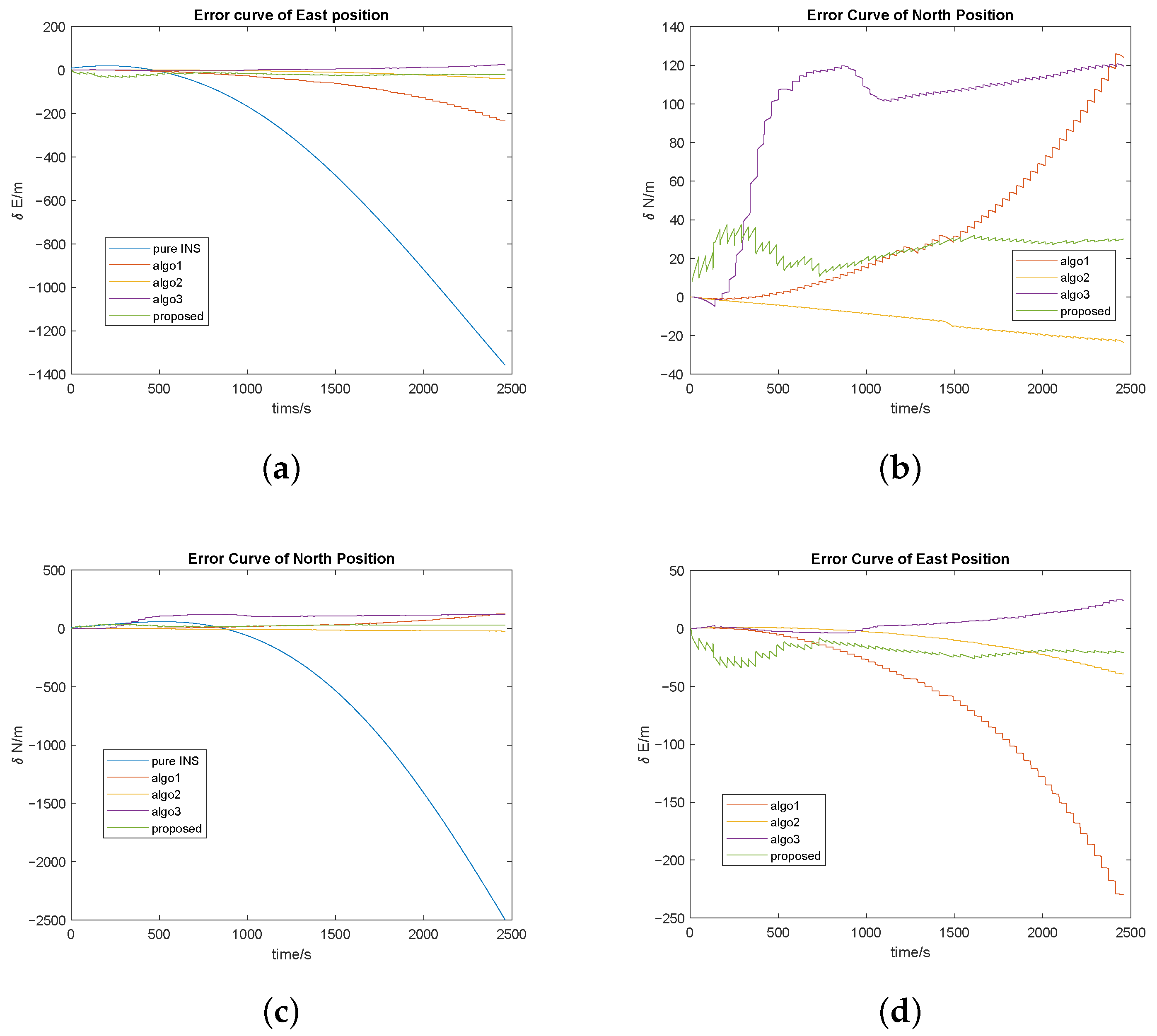
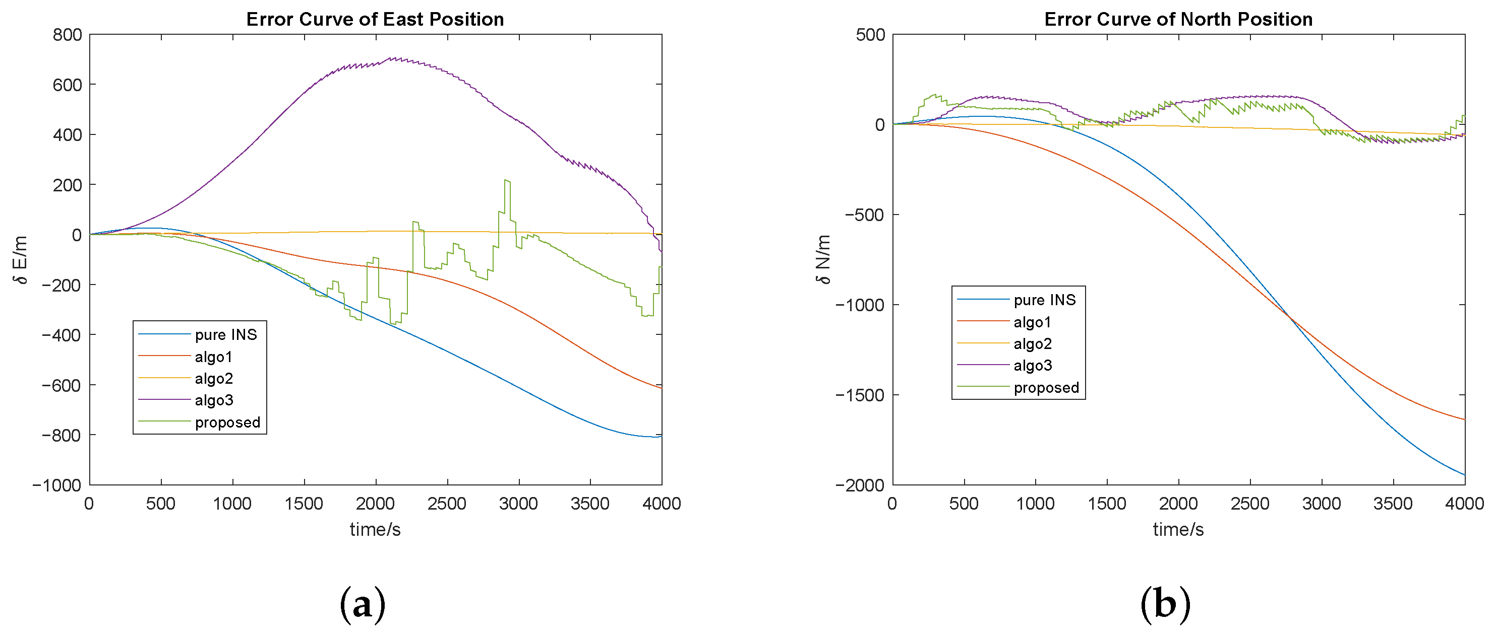
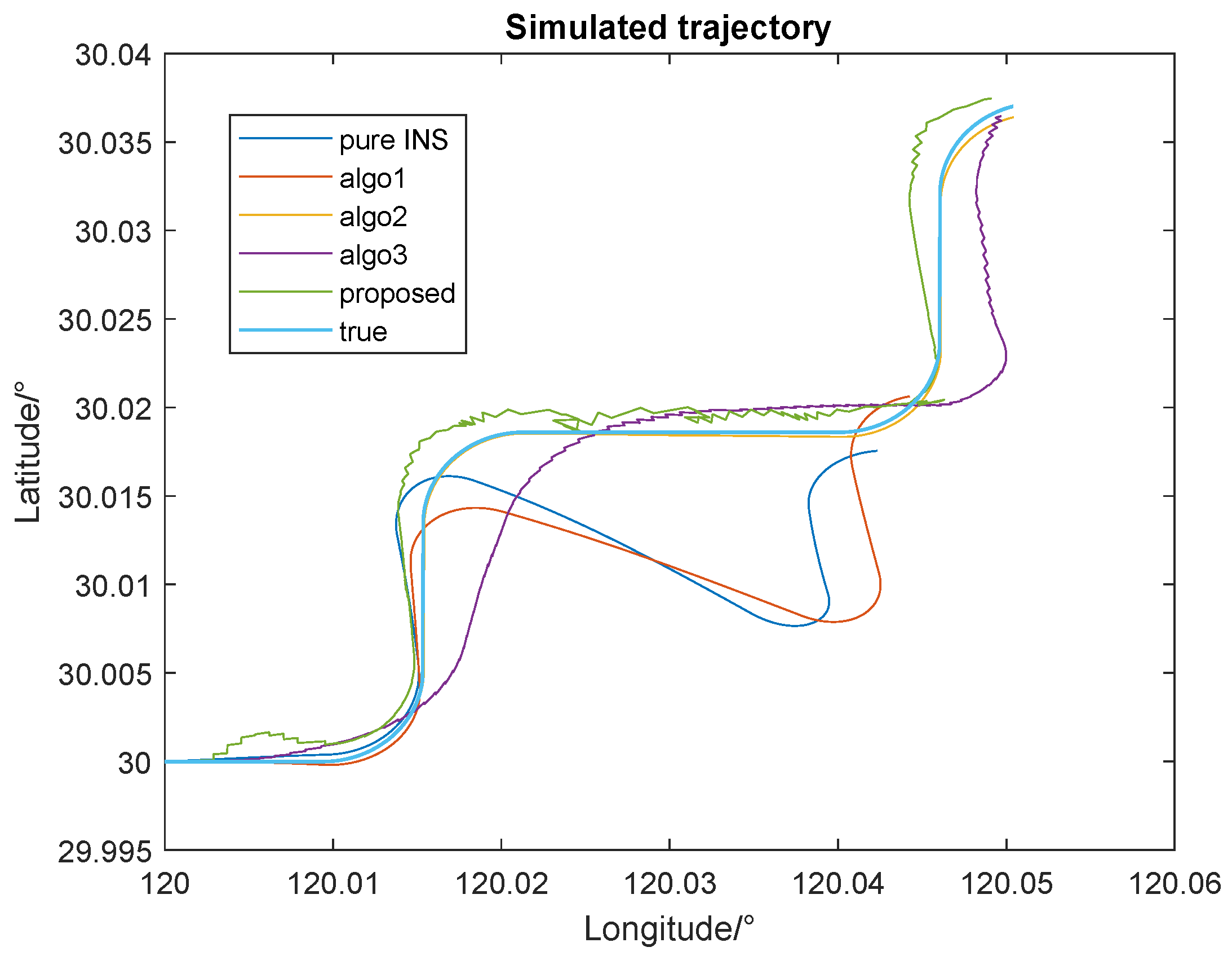
4.2. Performance Comparison

To verify the navigation performance of the proposed method, we compare it in the same conditions with INS only, the INS/APS tightly coupled model with range-only measurement (algo1), the algorithm (algo2 with DVL) proposed in [16] and the synthetic baseline algorithm (algo3) which is proposed in [14]. The configuration is shown in

Table 6. Simulation configuration in performance comparison.

Parameter	Value
Number of hydrophone elements	10
Spatial interval of elements	5 m
Sample rate of hydrophone	4000 Hz
Sample rate of IMU	100 Hz
Duration of simulation	2460 s, 4000 s
Times of repetition	1
Initial distance between the beacon and the vehicle	50 km
Initial bearing angle	0${}^{\circ }$
Voyage speed	2 m/s
Accuracy of depth sensor	0.1 m
Accuracy of Compass	0.1${}^{\circ }$
SNR	−30 dB
Frequency of narrowband signal	100 Hz
Broadband signal (a period)	LFM ($130\sim 230$ Hz, 40 s)
${\mathbf{Q}}_k$	$Diagonal({10}^{-7},{10}^{-8},{10}^{-6},{10}^{-9},{10}^{-4},{10}^{-5},{10}^{-6})$
${\mathbf{R}}_k$	$I_{21\times 21}\times {10}^{-3}$
${\mathbf{P}}_0$	$Diagonal(0.1,0.01,0.01,0.01,0.01,0.01,{10}^{-8})$
${\mathbf{Qn}}_k$	$Diagonal({10}^{-10},{10}^{-10},{10}^{-8},{10}^{-8},{10}^{-10},{10}^{-10},{10}^{-10},{10}^{-12},$ ${10}^{-12},{10}^{-12},{10}^{-12},{10}^{-12},{10}^{-12},{10}^{-12})$
${\mathbf{Rn}}_k$	$Diagonal({10}^4,{10}^4)$
${\mathbf{Pn}}_0$	$Diagonal({10}^{-8},{10}^{-8},{10}^{-6},{10}^{-6},{10}^{-8},{10}^{-8},{10}^{-10},{10}^{-8},{10}^{-8},$ ${10}^{-8},{10}^{-10},{10}^{-10},{10}^{-10},{10}^{-10})$

. The simulating trajectory is shown in Figure 8. The simulation results are shown in Figure 9.

The average root means square error (ARMSE) after the simulation of every algorithm are listed in

Table 7. The ARMSE of each algorithm.

	East ARMSE (m)	North ARMSE (m)	Total (m)
INS Only	608.48	966.39	1142.00
Algo1	91.65	49.58	104.20
Algo2	15.67	14.43	21.30
Algo3	9.15	102.31	102.72
Proposed	20.47	25.77	32.91

. From the results, we can see that with the aid of the acoustic positioning system, the navigation accuracy of three integrated algorithms are improved apparently. They all effectively restrict the accumulating error which is caused by the drift of inertial sensors. From Table 7, algo2 and the proposed algorithm are much better than algo1. Although the ARMSE in the east direction of algo3 is smaller than other algorithms, the majority of the positioning error lies in the north direction. The total ARMSE of algo1 and algo3 are on the same level. The accuracy of the proposed method is relatively worse than the algo2. It should be noted that algo2 is an integrated navigation scheme that combines INS, DVL, and OWTT measurements, while the proposed method only uses information from INS and OWTT. Despite this difference, the proposed algorithm performs nearly so well as algo2 when the AUV follows the trajectory shown in Figure 8. The results clearly demonstrate the superiority of the proposed algorithm over algo1 and 3 in INS/OWTT-based navigation.

Figure 10 shows another type of simulated trajectory, for which the constant-velocity model was found to be unsuitable due to a 40-s time interval between each state.

Table 8. The ARMSE of each algorithm.

	East ARMSE (m)	North ARMSE (m)	Total (m)
INS Only	453.30	947.77	1050.69
Algo1	265.25	880.55	919.63
Algo2	8.05	26.10	27.32
Algo3	442.96	103.11	454.80
Proposed	155.89	79.39	174.95

displays the ARMSE of each algorithm. Error curves and the AUV’s trajectory for the navigation results generated by pure inertial navigation, algo1, algo2, algo3, and the proposed algorithm are shown in Figure 11 and Figure 12, respectively. The results indicate that the proposed algorithm has higher accuracy than algo1, algo3, and the pure inertial cases. However, compared to algo2, which is aided by DVL and APS, it cannot achieve the same level of accuracy in this case.

5. Field-Experimental Design

The field experiment is required if we want to verify the real performance of the proposed algorithm. Currently, the field experiment has not been carried out; however, the design of the field experiment is presented.

5.1. Experimental Requirements

Firstly, the field experiment should be conducted in the ocean, and the area should be at least 2500 nmile square. An AUV is needed as an experiment platform. The AUV should be equipped with a hydrophone array, GNSS receiver, IMU, an on-vehicle computer, DVL and so on. The AUV should automatically travel through the pre-set route, in the meantime, record the data including IMU’s data, hydrophones’ data and navigation results. In addition, according to the field experiments in previous research, the number of elements of the hydrophone array should be more than four.

Secondly, a high-power acoustic beacon is needed as the signal transmitter. The bandwidth of the beacon should at least cover 50 Hz to 1000 Hz. The beacon should be programmable so that the researchers can freely set the signal’s format. In addition,  the maximum source level of the beacon should be no less than 180 dB.

Last but not least, a high-accuracy LBL system is needed. This system should be deployed near the AUV and the effective range of the LBL system should cover the trajectory of the AUV. This system is served as a reference system which provides the benchmark for the experiment.

5.2. Experimental Procedure

Before the field experiment, several position points and areas should be preset which are: the voyage area of the AUV where the LBL system is deployed; a point locates 50 km away from the voyage area; a point locates 100 km away from the voyage area; a point locates 150 km away from the voyage area. The whole procedure of the experiment is as follows.

• Two ships carry the AUV and the beacon, respectively, and reach the preset positions. The beacon should be firstly at the 50 km point. Then, the AUV and the beacon are released into the ocean.
• The beacon plays the acoustic signal (single-frequency signal + wide bandwidth ranging signal). Note that the bandwidth of the signal should not overlap the LBL’s bandwidth. In the meantime, the AUV voyages along with the preset trajectory (the velocity of the AUV should be approximately constant and no more than 4 m/s). The AUV records the sensors’ data and the LBL positions. The whole process should last at least one hour. The 50 km-point test repeats three times.
• Then, the beacon should be deployed at the 100 km-point and play the same signal. The AUV repeats the same process as 50 km-point test.
• Repeat the same process for the 150 km-point test.
• Collect the data recorded by the AUV. Post-process the IMU’s data and the hydrophones data using the conventional single beacon method, range-only tightly coupled method, some state-of-the-art single beacon methods and the proposed method, respectively. Compare every method’s results with LBL data. Attention should be attached to three values: the average positioning error, the system available time, and the effective range of the acoustic aid.

6. Discussion and Conclusions

This work focuses on improving the accuracy of underwater navigation in long-range and low-SNR conditions. To achieve this target, a new scheme of INS/APS integrated navigation is proposed. This method combines passive synthetic aperture detection and tightly coupled navigation. The signal for range and bearing measurement is a composite signal, which contains a single-frequency signal and a modulated signal. We design a DOA/range estimator and a tightly coupled INS/APS integrated estimator based on UKF. The two estimators’ architecture is proven to be slighter in computation compared with one estimator’s architecture. The motion restriction simulation reveals that the accuracy of the proposed method varies from the relative direction between the voyaging direction and the beacon. Meanwhile, the simulation results shows its superiority compared with other INS/APS integrated navigation algorithms and even performs as good as the algorithm aided with DVL.

Although research has made significant progress in proposing new algorithms, there are still limitations that need to be addressed. Firstly, field experiments are necessary to verify the proposed algorithm. Secondly, the algorithm is not suitable for single hydrophone conditions. Thirdly, compared to conventional INS/APS integrated navigation, the proposed algorithm requires higher computational resources, necessitating more advanced on-board hardware.

Future research of this work will focus on these aspects:

• The practical experiments verification. The real environment will be much more complex. Some parameters which are suitable for simulation may not be the same case in the real world. Practical experiments will help improve the model and verify its real performance.
• The implementation of auto-tuning and adaptive data-fusion algorithm will be also important in the next step of the work. Although there are lots of KF-based adaptive data-fusion algorithms, most of them just introduce some new hyperparameters such as fading factors. So, it is still a game of tuning. We hope that we can design an adaptive estimator which can provide the appropriate UKF parameters based on the underwater environment.
• Generalize the model. The current model is established based on the constant velocity model. However, a more general model is needed, as the motion type of the underwater vehicle is required to be more flexible.
• A better updating strategy. During the research of this work, we find that the updating rate of each subsystem is different. Especially, the OWTT range measurement is much lower than others. This problem causes the fluctuation of estimation error. The error curve is saw-toothed because of the long updating period. On the other hand, due to the disturbance of ocean circumstances, we cannot guarantee a stable updating rate of OWTT data. We want to find some methods such as temporal predictions to eliminate such fluctuation when OWTT measurement is not available.

Further research of long-range underwater navigation without GNSS will make a contribution to deep-sea exploration, oceanic science, and flexible navy application.

References

1. Webster, S.E.; Lee, C.M.; Gobat, J.I. Preliminary results in under-ice acoustic navigation for seagliders in Davis Strait. In Proceedings of the 2014 Oceans, St. John’s, NL, Canada, 14–19 September 2014; pp. 1–5. [Google Scholar] [CrossRef]
2. Graupe, C.E.; van Uffelen, L.J.; Webster, S.E.; Worcester, P.F.; Dzieciuch, M.A. Preliminary results for glider localization in the Beaufort Duct using broadband acoustic sources at long range. In Proceedings of the OCEANS 2019 MTS/IEEE, Seattle, WA, USA, 27–31 October 2019; pp. 1–6. [Google Scholar] [CrossRef]
3. Webster, S.E.; Freitag, L.E.; Lee, C.M.; Gobat, J.I. Towards real-time under-ice acoustic navigation at mesoscale ranges. In Proceedings of the 2015 IEEE International Conference on Robotics and Automation (ICRA), Seattle, WA, USA, 26–30 May 2015; pp. 537–544. [Google Scholar] [CrossRef]
4. Stergiopoulos, S.; Sullivan, E.J. Extended towed array processing by an overlap correlator. J. Acoust. Soc. Am. 1989, 86, 158–171. [Google Scholar] [CrossRef]
5. Wang, Y.; Gong, Z.; Zhang, R. An improved phase correction algorithm in extended towed array method for passive synthetic aperture. Proc. Meet. Acoust. 2017, 30, 055007. [Google Scholar] [CrossRef]
6. Bee, T.P.; Siong, L.H.; Swee, C.C.; Passerieux, J.M. Extended Towed Array Measurement: Beam-domain phase estimation and coherent summation. In Proceedings of the OCEANS 2006—Asia Pacific, Singapore, 16–19 May 2006; pp. 1–6. [Google Scholar] [CrossRef]
7. Lim, H.S.; Tong, P.B.; Chia, C.S. Scenario Based Study of ETAM and FFTSA in Realistic Simulated Environment. In Proceedings of the OCEANS 2006—Asia Pacific, Singapore, 16–19 May 2006; pp. 1–7. [Google Scholar] [CrossRef]
8. Song, L.; Zhi-Xiang, Y. Influencing Factors of Passive Synthetic Aperture Technology Based on FFTSA. In Proceedings of the 2021 OES China Ocean Acoustics (COA), Harbin, China, 14–17 July 2021; pp. 955–960. [Google Scholar] [CrossRef]
9. Wang, Y.; Sun, G.C.; Wang, Y.; Zhang, Z.; Xing, M.; Yang, X. A High-Resolution and High-Precision Passive Positioning System Based on Synthetic Aperture Technique. IEEE Trans. Geosci. Remote. Sens. 2022, 60, 1–13. [Google Scholar] [CrossRef]
10. Sullivan, E.J. Model-Based Processing for Underwater Acoustic Arrays; SpringerBriefs in Physics; Springer: Cham, Switzerland, 2015. [Google Scholar] [CrossRef]
11. Yang, T.C. Source depth estimation based on synthetic aperture beamfoming for a moving source. J. Acoust. Soc. Am. 2015, 138, 1678–1686. [Google Scholar] [CrossRef] [PubMed]
12. Fischell, E.M.; Rypkema, N.R.; Schmidt, H. Relative Autonomy and Navigation for Command and Control of Low-Cost Autonomous Underwater Vehicles. IEEE Robot. Autom. Lett. 2019, 4, 1800–1806. [Google Scholar] [CrossRef]
13. Kepper, J.H.; Claus, B.C.; Kinsey, J.C. A Navigation Solution Using a MEMS IMU, Model-Based Dead-Reckoning, and One-Way-Travel-Time Acoustic Range Measurements for Autonomous Underwater Vehicles. IEEE J. Ocean. Eng. 2019, 44, 664–682. [Google Scholar] [CrossRef]
14. Larsen, M. Synthetic long baseline navigation of underwater vehicles. In Conference Proceedings (Cat. No.00CH37158), Proceedings of the OCEANS 2000 MTS/IEEE Conference and Exhibition, Providence, RI, USA, 11–14 September 2000; Volume 3, pp. 2043–2050. [CrossRef]
15. Casey, T.; Guimond, B.; Hu, J. Underwater Vehicle Positioning Based on Time of Arrival Measurements from a Single Beacon. In Proceedings of the OCEANS 2007, Vancouver, BC, Canada, 29 September–4 October 2007; pp. 1–8. [Google Scholar] [CrossRef]
16. Webster, S.E.; Eustice, R.M.; Singh, H.; Whitcomb, L.L. Advances in single-beacon one-way-travel-time acoustic navigation for underwater vehicles. Int. J. Robot. Res. 2012, 31, 935–950. [Google Scholar] [CrossRef]
17. Qin, H.D.; Yu, X.; Zhu, Z.B.; Deng, Z.C. A variational Bayesian approximation based adaptive single beacon navigation method with unknown ESV. Ocean. Eng. 2020, 209, 107484. [Google Scholar] [CrossRef]
18. Rypkema, N.R.; Fischell, E.M.; Schmidt, H. One-way travel-time inverted ultra-short baseline localization for low-cost autonomous underwater vehicles. In Proceedings of the 2017 IEEE International Conference on Robotics and Automation (ICRA), Singapore, 29 May–3 June 2017; pp. 4920–4926. [Google Scholar] [CrossRef]
19. Rypkema, N.R.; Fischel, E.M.; Schmidt, H. Closed-Loop Single-Beacon Passive Acoustic Navigation for Low-Cost Autonomous Underwater Vehicles. In Proceedings of the 2018 IEEE/RSJ International Conference on Intelligent Robots and Systems (IROS), Madrid, Spain, 1–5 October 2018; pp. 641–648. [Google Scholar] [CrossRef]
20. Sun, S.; Zhang, X.; Zheng, C.; Zhao, C.; Fu, J. Underwater asynchronous navigation using single beacon based on the phase difference. Appl. Acoust. 2021, 172, 107546. [Google Scholar] [CrossRef]
21. Zhao, W.; Zhao, H.; Liu, G.; Zhang, G. ANFIS-EKF-Based Single-Beacon Localization Algorithm for AUV. Remote. Sens. 2022, 14, 5281. [Google Scholar] [CrossRef]
22. De Palma, D.; Arrichiello, F.; Parlangeli, G.; Indiveri, G. Underwater localization using single beacon measurements: Observability analysis for a double integrator system. Ocean. Eng. 2017, 142, 650–665. [Google Scholar] [CrossRef]
23. Paull, L.; Saeedi, S.; Seto, M.; Li, H. AUV Navigation and Localization: A Review. IEEE J. Ocean. Eng. 2014, 39, 131–149. [Google Scholar] [CrossRef]
24. Leonard, J.J.; Bahr, A. Autonomous Underwater Vehicle Navigation. In Springer Handbook of Ocean Engineering; Dhanak, M.R., Xiros, N.I., Eds.; Springer Handbooks; Springer: Cham, Switzerland, 2016; pp. 341–358. [Google Scholar] [CrossRef]
25. Chen, Y.; Zheng, D.; Miller, P.A.; Farrell, J.A. Underwater Inertial Navigation with Long Baseline Transceivers: A Near-Real-Time Approach. IEEE Trans. Control Syst. Technol. 2016, 24, 240–251. [Google Scholar] [CrossRef]
26. Claus, B.; Kepper IV, J.H.; Suman, S.; Kinsey, J.C. Closed-loop one-way-travel-time navigation using low-grade odometry for autonomous underwater vehicles. J. Field Robot. 2018, 35, 421–434. [Google Scholar] [CrossRef]
27. Zhang, L.; Hsu, L.T.; Zhang, T. A Novel INS/USBL Integrated Navigation Scheme Via Factor Graph Optimization. IEEE Trans. Veh. Technol. 2022, 71, 1. [Google Scholar] [CrossRef]
28. Noureldin, A.; Karamat, T.B.; Georgy, J. Fundamentals of Inertial Navigation, Satellite-Based Positioning and Their Integration; Springer: Berlin/Heidelberg, Germany, 2013. [Google Scholar] [CrossRef]
29. Morin, P.; Eudes, A.; Scandaroli, G. Uniform Observability of Linear Time-Varying Systems and Application to Robotics Problems. In Proceedings of the Geometric Science of Information; Lecture Notes in Computer Science; Nielsen, F., Barbaresco, F., Eds.; Springer: Cham, Switzerland, 2017; pp. 336–344. [Google Scholar] [CrossRef]
30. Tuna, S.E. Sufficient Conditions on Observability Grammian for Synchronization in Arrays of Coupled Linear Time-Varying Systems. IEEE Trans. Autom. Control 2010, 55, 2586–2590. [Google Scholar] [CrossRef]
31. NIJMEIJER, H. Observability of autonomous discrete time non-linear systems: A geometric approach. Int. J. Control 1982, 36, 867–874. [Google Scholar] [CrossRef]
32. Batista, P.; Silvestre, C.; Oliveira, P. Single range aided navigation and source localization: Observability and filter design. Syst. Control Lett. 2011, 60, 665–673. [Google Scholar] [CrossRef]
33. Batista, P.; Silvestre, C.; Oliveira, P. Optimal position and velocity navigation filters for autonomous vehicles. Automatica 2010, 46, 767–774. [Google Scholar] [CrossRef]
34. Chen, Z.; Jiang, K.; Hung, J. Local observability matrix and its application to observability analyses. In Proceedings of the IECON ’90: 16th Annual Conference of IEEE Industrial Electronics Society, Pacific Grove, CA, USA, 27–30 November 1990; Volume 1, pp. 100–103. [Google Scholar] [CrossRef]
35. Northardt, T. Observability Criteron Guidance for Passive Towed Array Sonar Tracking. IEEE Trans. Aerosp. Electron. Syst. 2022, 58, 3578–3585. [Google Scholar] [CrossRef]
36. Wan, E.; Van Der Merwe, R. The unscented Kalman filter for nonlinear estimation. In Proceedings of the IEEE 2000 Adaptive Systems for Signal Processing, Communications, and Control Symposium (Cat. No.00EX373), Lake Louise, AL, Canada, 1–4 October 2000; pp. 153–158. [Google Scholar] [CrossRef]
37. Kepper, J.H.; Claus, B.C.; Kinsey, J.C. MEMS IMU and one-way-travel-time navigation for autonomous underwater vehicles. In Proceedings of the OCEANS 2017, Aberdeen, UK, 19–22 June 2017; pp. 1–9. [Google Scholar] [CrossRef]
38. Groves, P. Principles of GNSS, Inertial, and Multisensor Integrated Navigation Systems, 2nd ed.; Artech House Publishers: London, UK, 2013. [Google Scholar]
39. Jiang, J.; Yu, F.; Lan, H.; Dong, Q. Instantaneous Observability of Tightly Coupled SINS/GPS during Maneuvers. Sensors 2016, 16, 765. [Google Scholar] [CrossRef] [PubMed]
40. Rhee, I.; Abdel-Hafez, M.; Speyer, J. Observability of an integrated GPS/INS during maneuvers. IEEE Trans. Aerosp. Electron. Syst. 2004, 40, 526–535. [Google Scholar] [CrossRef]
Figure 1. The block diagram of the underwater integrated navigation system.
Remotesensing 15 01854 g001
Figure 2. The basic application scenario of the moving hydrophone array. If the distance between the moving hydrophone array is long enough ( d i s t a n c e > ( N × d ) 2 / λ ), the reaching angle θ of the signal at each element can be viewed as the same. So, θ is defined as the bearing angle between array and beacon. The interval between adjacent elements is d. N is the number of elements. λ is the wavelength of the signal.
Remotesensing 15 01854 g002
Figure 3. The relation of the distance between the vehicle and the beacon at two different moments.
Remotesensing 15 01854 g003
Figure 4. The histogram of the error in the acoustic OWTT range estimates.
Remotesensing 15 01854 g004
Figure 5. The block diagram of the simulation process.
Remotesensing 15 01854 g005
Figure 6. The variation in accuracy of bearing estimation when initial bearing is different.
Remotesensing 15 01854 g006
Figure 7. The variation in accuracy of range estimation when initial bearing is different.
Remotesensing 15 01854 g007
Figure 8. The simulated trajectory.
Remotesensing 15 01854 g008
Figure 9. (a) Error curve of INS only, algo1, algo2, algo3 and the proposed method in east position; (b) error curve of algo1, algo2, algo3, and the proposed method in east position; (c) error curve of INS only, algo1, algo2, algo3, and the proposed method in north position; (d) error curve of algo1, algo2, algo3, and the proposed method in north position.
Remotesensing 15 01854 g009
Figure 10. The simulating trajectory.
Remotesensing 15 01854 g010
Figure 11. (a) Error curve of INS only, algo1, algo2, algo3, and the proposed method in east position; (b) error curve of algo1, algo2, algo3, and the proposed method in east position.
Remotesensing 15 01854 g011
Figure 12. The comparison of trajectories calculated by different algorithms.
Remotesensing 15 01854 g012