Screening Image Features of Collapsed Buildings for Operational and Rapid Remote Sensing Identification

Abstract

The accurate detection of collapsed buildings is of great significance for post-disaster rescue and reconstruction. High-resolution optical images are important data sources for identifying collapsed buildings, and the identification accuracy mainly depends on the features extracted from the images. However, existing research lacks a comprehensive screening and general evaluation of the ability of remote sensing features to detect collapsed buildings, and there is still a considerable gap in the operational process of rapid identification of collapsed buildings in remote sensing. Based on 2630 pairs of building samples distributed in 6 regions worldwide, this study evaluated the ability of 25 remote sensing features (including spectral and spatial features) to detect collapsed buildings and select the most capable ones. Then, we test the application effect of selected features in identifying collapsed buildings on large-scale remote sensing images. Based on the two experiments above, an operational process for rapid identification of collapsed buildings was suggested. The result shows that Homogeneity, Energy, Local Entropy, Local Standard Deviation, and Gradient can effectively and stably distinguish collapsed buildings from non-collapsed buildings (Jeffries-Matusita distances are greater than 1.59 and Transformed Divergences are greater than 1.60) and have high recognition accuracy for collapsed buildings on large-scale remote sensing images (F₁-scores are 0.71–0.94). In addition, Contrast, Local Coefficient of Variation, Edge Density, and Global Entropy can also distinguish collapsed buildings from non-collapsed buildings at a normal level (Jeffries-Matusita distances are 1.14–1.28, and Transformed Divergences are 1.24–1.48), while Gradient Orientation Entropy, Fractal Dimension, Local Binary Patterns, Edge, Local Mean, Correlation, Gradient Orientation Standard Deviation, Global Coefficient of Variation, Gabor feature, Local Moran’I, and six spectral features have relatively weak abilities (Jeffries-Matusita distances are less than 0.73, and Transformed Divergences are less than 1.07). The selected remote sensing features can support rapid identification of potential collapsed building areas from post-disaster remote sensing images.

1. Introduction

Building collapse caused by disasters is an important damage to lives and properties. Rapid identification of collapsed buildings is of great significance for post-disaster rescue [1] and reconstruction [2]. In recent years, remote sensing has become an important method of obtaining building damage information because of its advantages of non-contact, low cost, wide field of view, and fast response [3]. Due to the urgency of post-disaster rescue, it is necessary to make the process of remote sensing identification of collapsed buildings operationalized so that we can rapidly identify collapsed buildings while maintaining high recognition accuracy.

Remote sensing identification essentially involves the following processes: data collection → feature extraction → feature selection → target identification using an appropriate classification method. The current methods for remote sensing identification mainly include traditional machine learning methods and deep learning methods, both of which essentially follow the process mentioned above. The deep learning methods avoid manual feature extraction and feature selection [4,5,6], but they require a large number of samples for training [7], which are limited in the case of collapsed buildings [8]. Although methods like data augmentation [9], transfer learning [8,10], or pseudo-labeled training sample production [11] could alleviate this problem, they all rely on the samples from the study area. Due to the small sample volume, it is easy to suffer from the uneven distribution of training samples, which affects the training accuracy of the model [8]. Therefore, current deep learning methods are still unable to meet the operationalization needs of rapid identification of collapsed buildings after disasters. In contrast, traditional machine learning methods do not require as many samples, and the effectiveness of their identification largely depends on the features used. The enhancement in either feature extraction or feature selection can contribute to improving the accuracy of collapsed building recognition. However, this study primarily focuses on feature selection.

There have been many features used for remote sensing recognition of collapsed buildings in previous studies. For example, Ye et al. [12] used texture and local spatial statistical features to identify collapsed buildings in the post-earthquake images of the 2015 Nepal earthquake; Zeng et al. [13] used grayscale mean and inverse different moment to identify collapsed buildings in post-earthquake images of Haiti and Yushu; Ye et al. [14] used local Moran’I, texture, and gradient to identify collapsed buildings in post-earthquake images of the Yushu earthquake; Sumer et al. [15] used grayscale values and gradient to identify collapsed buildings in post-earthquake images of the Kocaeli earthquake. The features used for collapsed building identification in previous studies include spectral features [16,17], Entropy, Coefficient of Variation, Local Mean, Local Standard Deviation, Local Moran’I [12,14], Gradient, Gradient Orientation [14,18], Edge, Edge Density [19], Gray Level Co-Occurrence Matrix (GLCM) [19,20], Local Binary Patterns (LBP), Fractal feature [21], and Gabor feature [21], etc. These features can be summarized into spectral features and spatial features (Figure 1), where spectral features include original bands and their derived features, and spatial features include spatial statistical features, gradient and edge features, and texture features. The research mentioned above has achieved good recognition results for collapsed buildings in specific areas, but there has been no study on how to select the optimal features. Instead, several features were directly used for identification based on prior knowledge, making the individual roles of these features unclear in the process. Furthermore, existing studies are all case studies conducted in a certain area, so it is still unknown whether the features can be equally applicable in other regions. In summary, although many features have been used for the recognition of collapsed buildings, their recognition ability and transferability have not been widely evaluated, and there is a lack of theoretical guidance on which features should be used for practical identification work. Therefore, there is still a gap in the operational process of rapid recognition of collapsed buildings in remote sensing.

Figure 1. Features of optical remote sensing images for identifying collapsed buildings.

This article is dedicated to screening out remote sensing features of collapsed buildings. By using a large building sample set collected from different regions around the world, this study evaluated the capability of 25 different features in detecting collapsed buildings and explored the optimal parameters for the features with good performance to make the best use of the features. For the features with good distinguishing ability for collapsed buildings, we test their effectiveness on the application test image set.

2. Data and Methodology

2.1. Data

2.1.1. Building Sample Set

The building sample set of this study includes 2630 pairs of building samples distributed in 6 regions worldwide. Each pair of building samples includes the pre- and post-collapse images of the same building. The samples are all visible-light images with a spatial resolution of about 0.5 m. Each sample is approximately 100 rows × 50 columns of pixels in size. The samples were selected from the xBD dataset [22] and the Open Data Program dataset (https://www.digitalglobe.com/ecosystem/open-data, accessed on 3 March 2023) of Maxar. The xBD dataset contains over 850,000 pairs of pre- and post-collapse building images as well as boundary vector data for pre-collapse buildings. In this study, a total of 2508 pairs of samples were selected through visual interpretation from the xBD dataset. The Open Data Program dataset provides remote sensing images before and after disaster events. A total of 122 pairs of pre- and post-collapse building samples were selected through visual interpretation, and the vector boundaries of pre-collapse buildings were manually outlined. Figure 2 shows image examples of some samples, and the detailed information of all samples is shown in Table 1.

Figure 2. Image examples of some samples. Note: The samples are within the blue boundaries. The pre-collapse samples are on the left, and the corresponding post-collapse samples are on the right.

Table 1. Detailed information on all building samples.

Image Shooting Location	Reasons and Timing of Building Collapse	Image Shooting Time	Number of Samples for Building Pairs
Bata (Equatorial Guinea—Litoral, 1.87°N, 9.77°E)	explosion (7 March 2021)	image before collapse: 7 August 2020 image after collapse: 9 March 2021	92
Beirut (Lebanon—Beirut, 33.87°N, 35.70°E)	explosion (4 August 2020)	image before collapse: 31 July 2020 image after collapse: 5 August 2020	30
Joplin (USA—Missouri, 37.10°N, 94.58°W)	tornado (22 March 2011)	image before collapse: 8 August 2009 image after collapse: 29 May 2011	1558
Moore (USA—Oklahoma, 35.33°N, 97.50°W)	tornado (20 May 2013)	image before collapse: 17 February 2013 image after collapse: 22 May 2013	594
Tuscaloosa (USA—Alabama, 33.2°N, 87.51°W)	tornado (27 April 2011)	image before collapse: 21 June 2006 image after collapse: 19 May 2011	277
Woolsey (USA—California, 34.06°N, 118.76°W)	wild fire (8 November 2018)	image before collapse: 23 October 2018 image after collapse: 18 November 2018	79

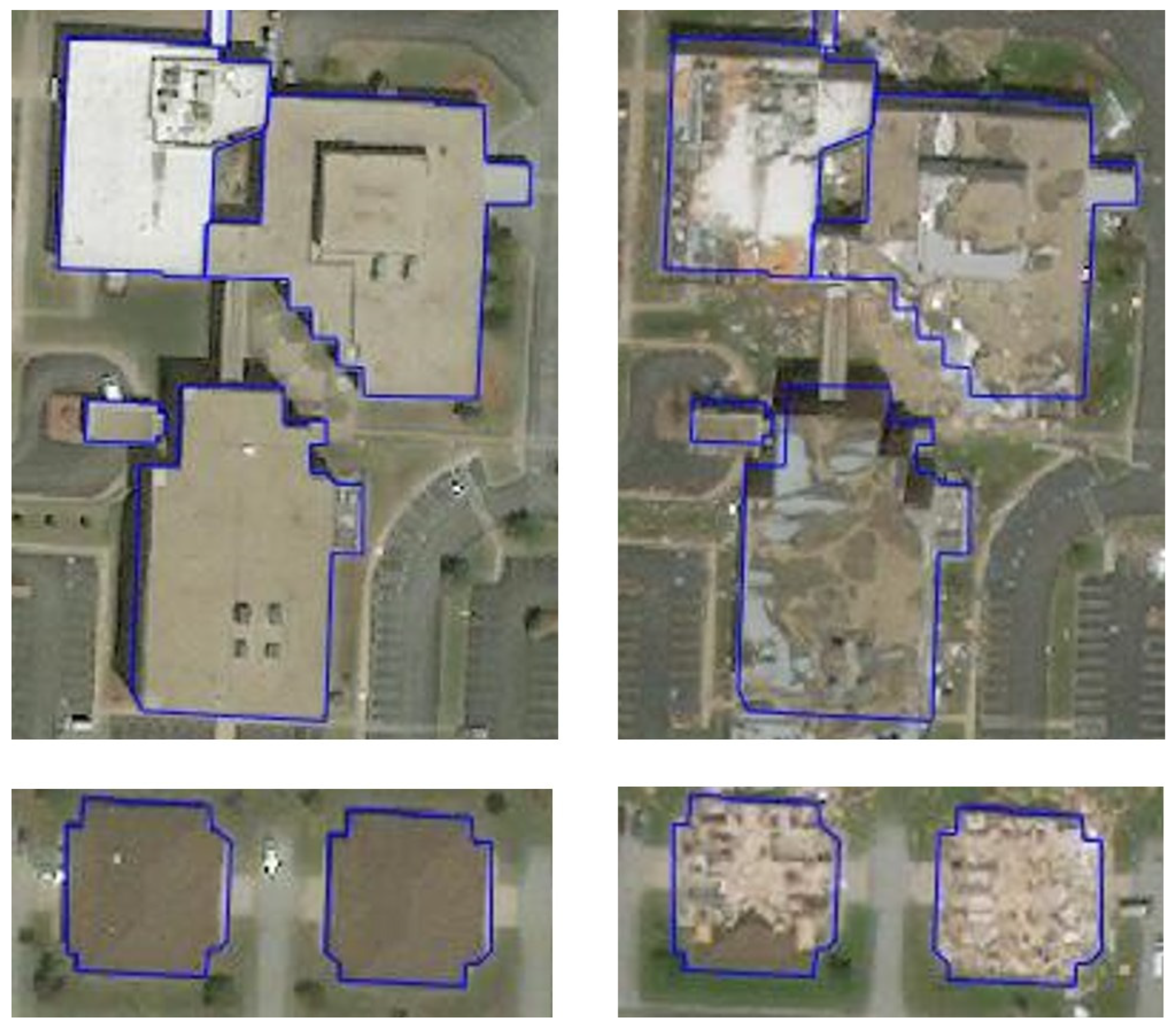
2.1.2. Application Test Image Set

The application test image set consists of three large-scale remote sensing images, namely post-disaster remote sensing images from Joplin (6408 rows × 4734 columns), Moore (13,560 rows × 10,019 columns), and Tuscaloosa (8431 rows × 5941 columns). These large-scale images are also visible light images derived from the Open Data Program dataset, with a spatial resolution of approximately 0.5 m. The application test image set is used to test the practical application ability of selected features in this study.

2.2. Methodology

Based on the building sample set, this study evaluated the ability of 25 features to distinguish collapsed buildings from non-collapsed buildings by two indicators (Jeffries-Matusita distance and Transformed Divergence) and explored the optimal parameters for the features with good performance. For the features with good distinguishing ability for collapsed buildings, we test their effectiveness on the application test image set.

2.2.1. Ability Evaluation of Features

The indicators used to evaluate the ability of features are Jeffries-Matusita distance (J-M distance) and Transformed Divergence (TD), which can measure the distance between collapsed building samples and non-collapsed building samples in the feature space. Both J-M distance and TD are in the range of 0 to 2, and the higher value indicates a better distinguishing ability of the feature.

The calculation formula for the J-M distance is shown in Equations (1) and (2):

$$J_{ij}=2\times \left(1-{\mathrm{e}}^{-B}\right)$$

(1)

$$B=\frac{{\left(U_i-U_j\right)}^{\mathrm{T}} \times {\left(\frac{{\sum }_i+{\sum }_j}{2}\right)}^{-1}\times \left(U_i-U_j\right)}{8}+\frac{\ln \left[\frac{\frac{1}{2}\times \left|{\sum }_i+{\sum }_j\right|}{\sqrt{\left(\left|{\sum }_i\right|\times \left|{\sum }_j\right|\right)}}\right]}{2}$$

(2)

where U is the mean vector of the sample, ∑ is the covariance matrix, and i and j are non-collapsed and collapsed building samples, respectively.

The calculation formula for TD is shown in Equation (3):

$$T{D}_{ij}=2\times \left(1-{\mathrm{e}}^{-D_{ij}/8}\right)$$

(3)

where D_ij is the divergence between non-collapsed and collapsed buildings, and its calculation formula is shown in Equation (4):

$$D_{ij}=\frac{{\mathrm{t}}_{\mathrm{r}}\left[\left({\sum }_i-{\sum }_j\right)\times \left({\sum }_j^{-1}-{\sum }_i^{-1}\right)\right]}{2}+\frac{{\mathrm{t}}_{\mathrm{r}}\left[\left({\sum }_i^{-1}-{\sum }_j^{-1}\right)\times \left(U_i-U_j\right)\times {\left(U_i-U_j\right)}^{\mathrm{T}}\right]}{2}$$

(4)

where U is the mean vector of the sample, ∑ is the covariance matrix, t_r[A] is the sum of diagonal elements in matrix A, and i and j are non-collapsed and collapsed building samples, respectively.

The extraction methods for various features are shown in Table 2.

Table 2. Feature Extraction methods.

Features	Calculation Methods
Red/Green/Blue	Calculate the mean of the red/green/blue band values of all pixels as the Red/Green/Blue feature of the building sample
Hue/Saturation/Intensity	Calculate the mean of hue/saturation/intensity values of the color space transformed sample image of all pixels as the Hue/Saturation/Intensity feature of the building sample
Global Entropy	Calculate the entropy of grayscale values of all pixels as the Global Entropy feature of the building sample
Global Coefficient of Variation	Calculate the coefficient of variation of grayscale values of all pixels as the Global Coefficient of Variation feature of the building sample
Local Mean	Using a specific-sized sliding window, calculate the mean/the standard deviation/the entropy/the coefficient of variation of the grayscale values in the window as the mean/the standard deviation/the entropy/the coefficient of variation value of the central pixel, and take the mean of the calculated values of all pixels as the Local Mean/the Local Standard Deviation/the Local Entropy/the Local Coefficient of Variation feature of the building sample
Local Standard Deviation
Local Entropy
Local Coefficient of Variation
Local Moran’I	Calculate the local Moran’I of each pixel, and take the mean of the local Moran’I values of all pixels as the Local Moran’I feature of the building sample
Gradient	Calculate the gradient value for every pixel by the Sobel operator, and take the mean of the gradient values of all pixels as the gradient feature of the building sample
Gradient Orientation Entropy	Calculate the gradient orientation for every pixel by the Sobel operator, and take the entropy for the gradient orientation values of all pixels as the Gradient Orientation Entropy feature of the building sample
Gradient Orientation Standard Deviation	Calculate the gradient orientation for every pixel by the Sobel operator, and take the standard deviation for the gradient orientation values of all pixels as the Gradient Orientation Standard Deviation feature of the building sample
Edge	Perform a convolution operation using the Laplacian operator, and take the mean value as the edge feature of the building sample
Edge Density	Perform a convolution operation using the Laplacian operator and apply thresholding segmentation to obtain edges. Calculate the density of edges in each pixel’s neighborhood, pixel by pixel. Afterwards, take the mean of the edge density values of all pixels as the edge density feature of the building sample
Contrast	Based on GLCM, calculate the contrast/correlation/energy/homogeneity value at each pixel and take the mean of the contrast/correlation/energy/homogeneity values of all pixels as the Contrast/Correlation/Energy/Homogeneity feature of the building sample
Correlation
Energy
Homogeneity
Local Binary Patterns (LBP)	Calculate LBP for every pixel with a certain radius, and take the mean of the LBP values of all pixels as the LBP feature of the building sample
Gabor Feature	Calculate the Gabor value for every pixel by Gabor filtering, and take the mean of the Gabor values of all pixels as the Gabor feature of the building sample
Fractal Dimension	Calculate the fractal dimension using the Box Counting Method as the Fractal Dimension feature of the building sample

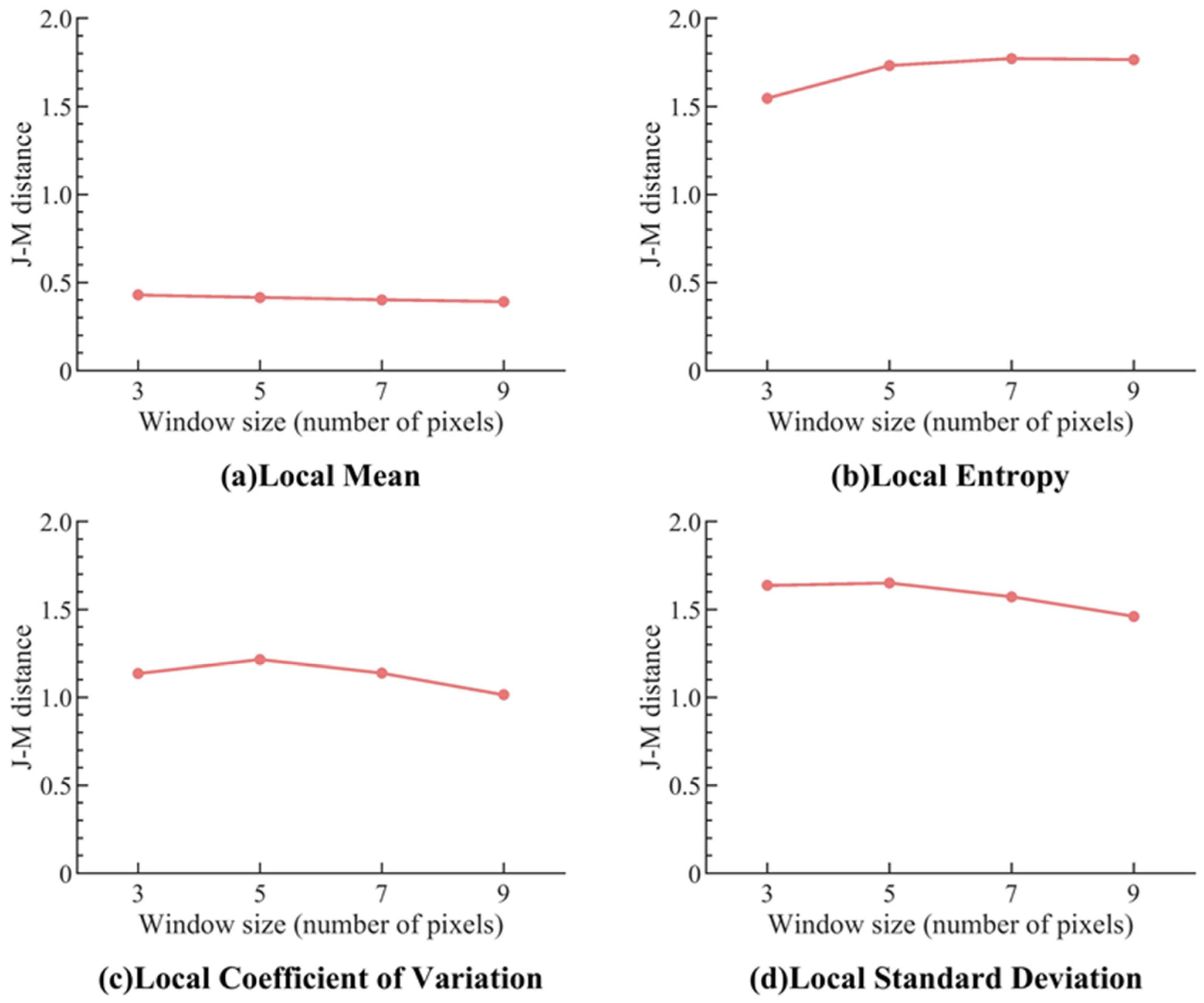
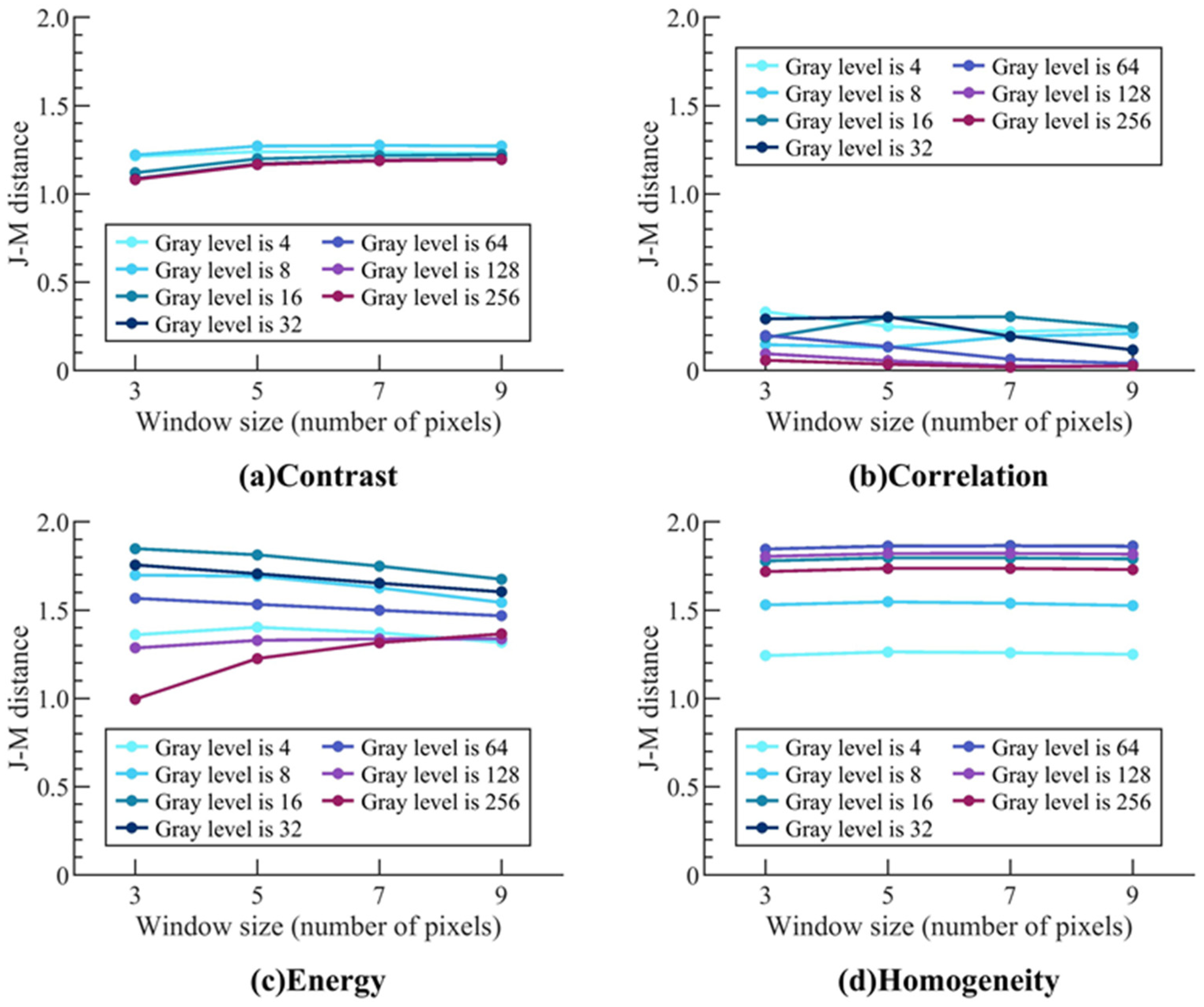
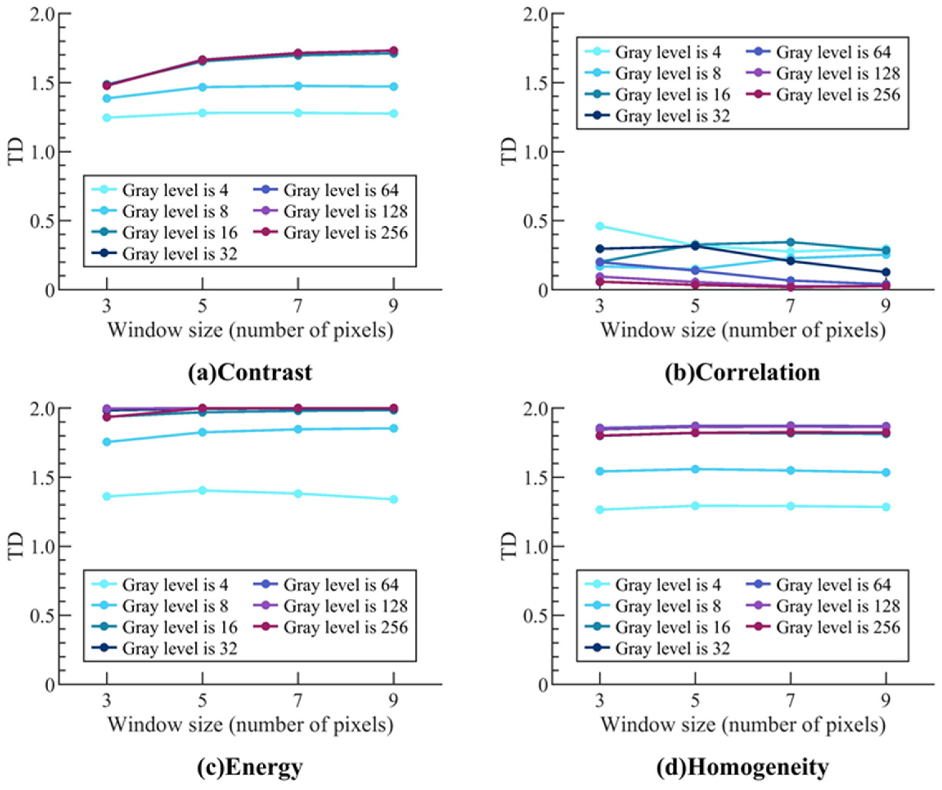
2.2.2. Optimization of Parameters in Feature Extraction

The Local Mean, Local Standard Deviation, Local Entropy, and Local Coefficient of Variation are easily affected by the window size. If the window size is too small, the feature cannot reflect the fragmentation of collapsed buildings, while the feature calculated by an oversized window may exaggerate the grayscale variations of non-collapsed buildings, resulting in a larger feature value than it should be. Therefore, an inappropriate window size may lead to a decrease in the ability of the feature to identify collapsed buildings. To explore the optimal window size, we calculated the above features under a series of window sizes and used J-M distance and TD as the measures of distinguishing ability.

Features calculated based on GLCM, such as Contrast, Correlation, Energy, and Homogeneity, are not only easily influenced by the window size but also by the gray level. If the gray level is not large enough, the difference between different fragments of collapsed buildings in grayscale will be diminished, so that the distinguishing ability for collapsed buildings of the feature can be weakened. If the gray level is huge, it can not only lead to excessive computation but also exaggerate the grayscale differences of non-collapsed buildings, and the extracted texture feature is more susceptible to noise. To explore the optimal combination of window size and gray level, we calculate the above features under a series combination and use J-M distance and TD as measures of distinguishing ability.

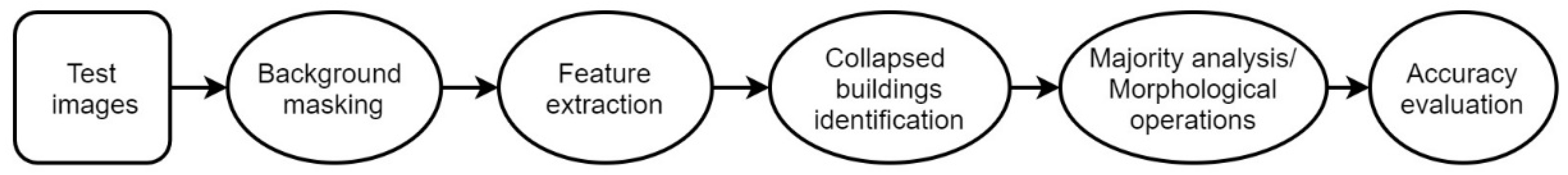
2.2.3. Assessment of the Application Effects of Selected Features

J-M distance and TD only illustrate the ability of the selected features to distinguish collapsed buildings from non-collapsed buildings in feature space, so we test the application effect of the features by using the images in the application test image set as an example. We used the thresholding method as the algorithm for extracting collapsed buildings instead of using a more complex machine learning algorithm, as it is the simplest and most intuitive method. Using the thresholding method can demonstrate that the extraction effect of collapsed buildings is derived from the contribution of the features rather than from the contribution of the classification algorithm. The technical flowchart for the assessment is shown in Figure 3.

Figure 3. A technical flowchart for assessing the application effects of selected features.

(1)

Collapsed building identification

Take Local Entropy as an example to illustrate the process of collapsed building identification. First, the vegetation index (the calculation formula is shown in Equation (5) [23]) was used to mask vegetation areas in the test image. Then, the Local Entropy of every pixel was calculated in the masked image, and the threshold method was used to extract collapsed buildings. For the segmented binary image, majority analysis and opening operations were used to eliminate small and meaningless patches, and the final identification result was obtained.

$$VI=2\times G-R-B$$

(5)

where VI represents the vegetation index, and R, G, and B represent the pixel values in the red, green, and blue bands of the image.

(2)

Accuracy evaluation

The confusion matrix calculated by randomly generated pixels is used to evaluate the accuracy of the identification of collapsed buildings. Approximately 1000 pixels were randomly generated from the non-collapsed and collapsed buildings of the classification result, respectively. Then, a confusion matrix is calculated by visually interpreting every random pixel. Based on the confusion matrix, precision, recall, and F₁-score were calculated as the recognition accuracy indicators.

Precision reflects the identification method’s ability to correctly identify collapsed buildings. Recall, on the other hand, reflects the identification method’s ability to avoid misidentifying non-collapsed buildings. The calculation formulas for precision and recall are shown in Equations (6) and (7).

$$precision=\frac{TP}{TP+FP}$$

(6)

$$recall=\frac{TP}{TP+FN}$$

(7)

where TP is the number of true positive samples, which is the number of the samples classified as collapsed buildings and, in fact, also collapsed buildings; FP is the number of false positive samples, which is the number of the samples classified as collapsed buildings but actually non-collapsed buildings; FN is the number of false negative samples, which refers to the number of samples classified as non-collapsed buildings but actually collapsed buildings.

The F₁-score takes both precision and recall into account and can comprehensively represent the accuracy of the classification results. The calculation formula is shown in Equation (8).

$${\mathrm{F}}_1=2\times \frac{precision\times recall}{precision+recall}$$

(8)

3. Results

3.1. Ability of 25 Features to Distinguish Collapsed Buildings from Non-Collapsed Buildings

There are significant differences in the ability to distinguish collapsed buildings from non-collapsed buildings of different features (Figure 4). Although the results of J-M distance and TD are not entirely consistent, they generally show the same patterns. The result shows Homogeneity, Energy, Local Entropy, Local Standard Deviation, and Gradient are more capable of distinguishing collapsed buildings from non-collapsed buildings (J-M distances are greater than 1.59, TDs are greater than 1.60), followed by Contrast, Local Coefficient of Variation, Edge Density, and Global Entropy (J-M distances are 1.14–1.28, TDs are 1.24–1.48). However, Gradient Orientation Entropy, Fractal Dimension, LBP, Edge, Local Mean, Correlation, Gradient Orientation Standard Deviation, Global Coefficient of Variation, Gabor feature, Local Moran’I, and six spectral features perform relatively poorly (J-M distances are less than 0.73, TDs are less than 1.07). There are also differences in the extraction times of different features; the results are presented in Appendix A.

Figure 4. (a) J-M distance and (b) TD of 25 features for non-collapsed and collapsed building samples. Note: Local std is Local Standard Deviation, Local CV is Local Coefficient of Variation, GO Entropy is Gradient Orientation Entropy, LBP is Local Binary Patterns, GO Std is Gradient Orientation Standard Deviation, and Global CV is Global Coefficient of Variation.

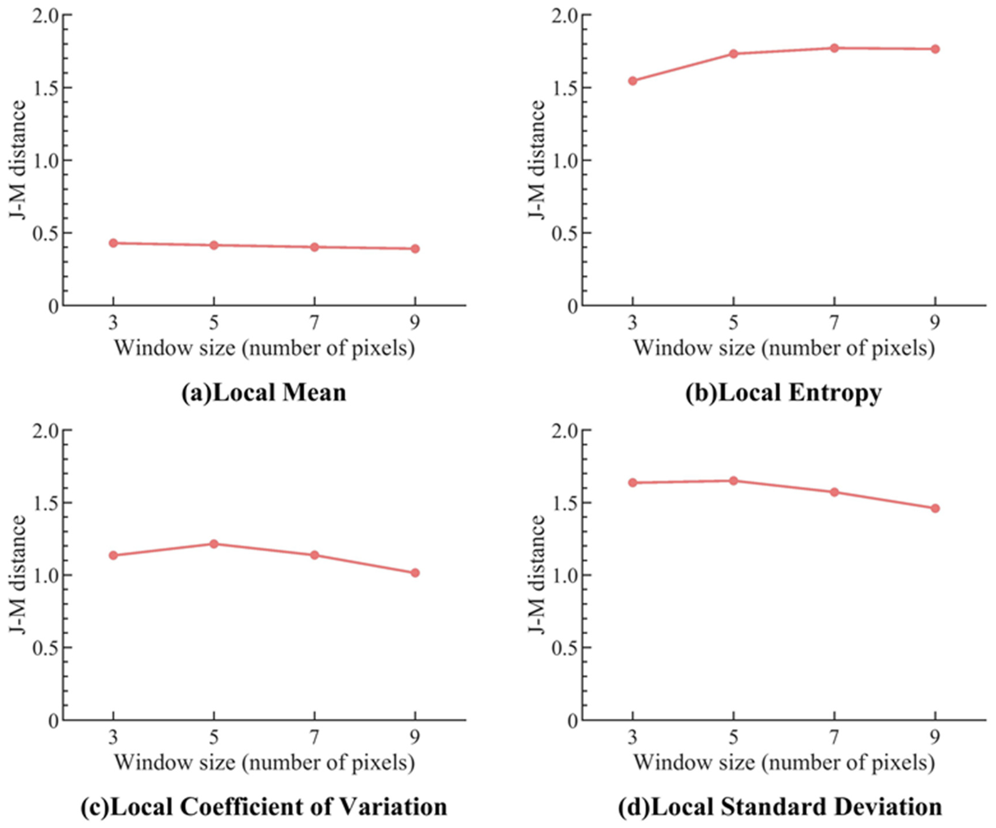
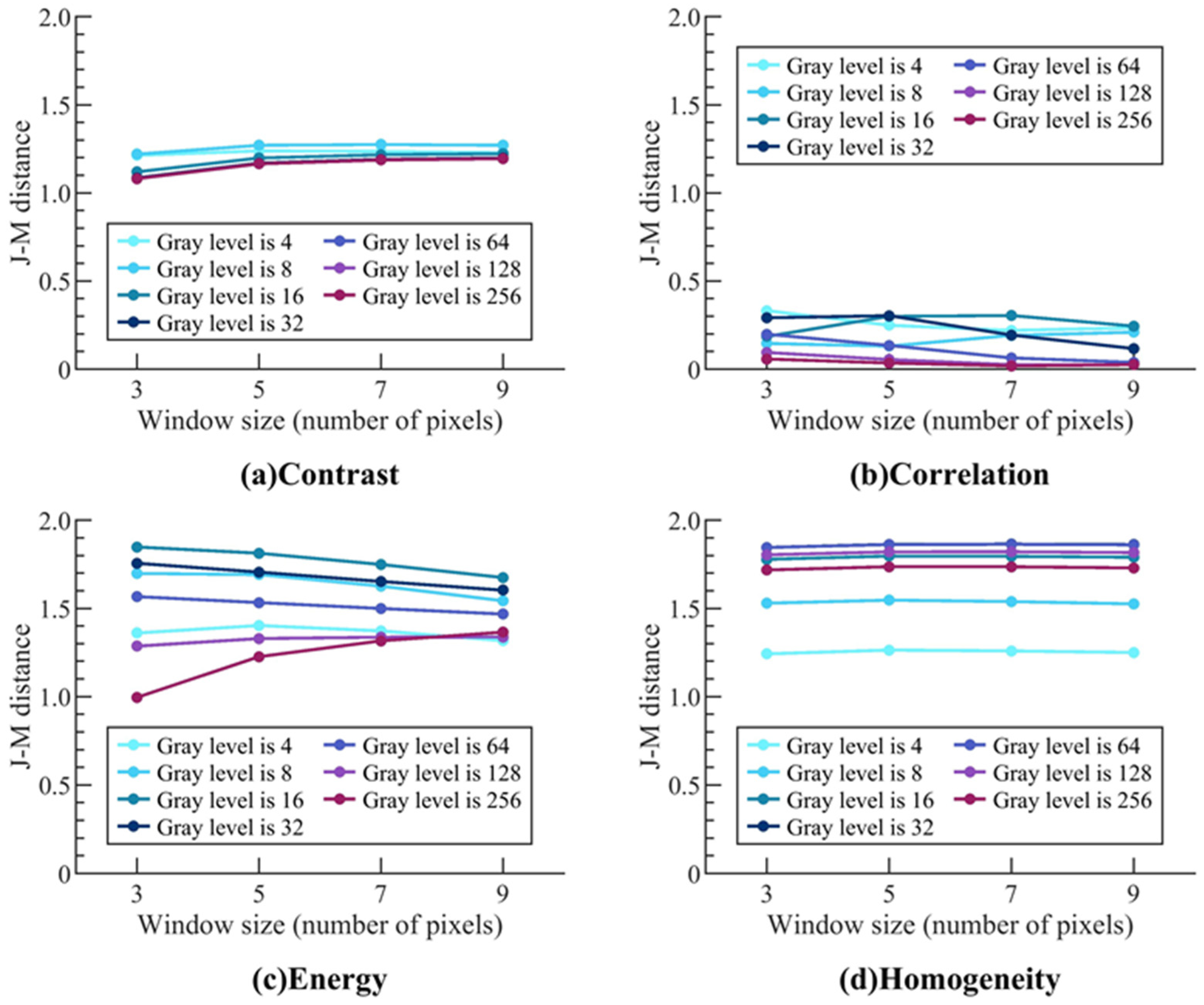
3.2. Optimal Parameters for Feature Extraction

The ability of Local Mean, Local Entropy, Local Coefficient of Variation, and Local Standard Deviation to distinguish collapsed buildings from non-collapsed buildings varies under different window sizes (Figure 5). Due to the same trend of variation in J-M distance and TD under different window sizes, only the results of J-M distance are shown here (the results of TD are presented in Appendix B). The Local Mean is not a well-performed feature and is not sensitive to changes in window size; therefore, it will not be discussed here. The J-M distances of the other three features exhibit the characteristic of initially increasing and then decreasing as the window size increases. Under the premise of a sample spatial resolution of around 0.5 m, the Local Entropy is optimal when the window size is 7 (i.e., around 3.5 m), and the Local Coefficient of Variation and Local Standard Deviation are optimal when the window size is 5 (i.e., around 2.5 m).

Figure 5. J-M distance of (a) Local Mean, (b) Local Entropy, (c) Local Coefficient of Variation, and (d) Local Standard Deviation under different window sizes.

Contrast, Correlation, Energy, and Homogeneity are calculated based on the GLCM; their ability is easily influenced by window size and gray level (Figure 6). The variation trends of J-M distance and TD are the same under different window sizes and slightly different under different gray levels, but this does not affect the optimal parameter results of each feature. Therefore, only the results of J-M distance are shown here (the results of TD are presented in Appendix B). Except for Correlation, which is not a well-performed feature, the J-M distances of Contrast, Energy, and Homogeneity all show a characteristic of initially increasing and then decreasing as the window size increases. The optimal window size is 5 or 7 (i.e., 2–4 m). The J-M distance of Contrast, Energy, and Homogeneity also shows a characteristic of initially increasing and then decreasing with the increase in gray level. The optimal gray level for Contrast is 8, for Energy is 16, and for Homogeneity is 32.

Figure 6. J-M distance of (a) Contrast, (b) Correlation, (c) Energy, and (d) Homogeneity under different window sizes and gray levels.

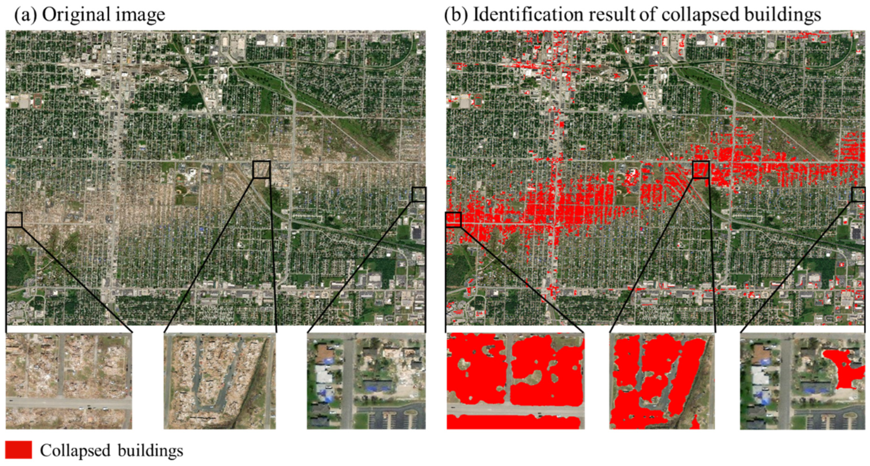
3.3. Application Ability of Selected Features

In practical application testing, the selected features (Local Entropy, Homogeneity, Energy, Local Standard Deviation, and Gradient) can effectively identify collapsed buildings (Table 3). The recall rates for identifying collapsed buildings from test images are all above 90%, while the precision rates are relatively low, ranging from 55% to 95%. The F₁ scores are between 0.71 and 0.94. Figure 7 shows the result of collapsed buildings identified in Joplin, and the feature used here is Gradient. It can be seen that almost all collapsed buildings have been extracted, with almost no missing areas. However, there are some non-collapsed areas misidentified as collapsed areas.

Table 3. The accuracy of collapsed building recognition when applying selected features to large-scale remote sensing images.

Features	Joplin			Tuscaloosa			Moore
	Precision (%)	Recall (%)	F1-Score	Precision (%)	Recall (%)	F1-Score	Precision (%)	Recall (%)	F1-Score
Local Entropy	94.50	93.20	0.94	70.10	96.29	0.81	84.00	97.45	0.90
Homogeneity	92.10	92.28	0.92	63.20	96.78	0.76	77.20	96.74	0.86
Energy	84.00	94.59	0.89	56.20	95.74	0.71	69.90	97.63	0.81
Local Standard Deviation	91.10	94.50	0.93	62.20	93.82	0.75	75.00	97.40	0.85
Gradient	79.80	91.30	0.85	59.80	94.77	0.73	62.30	97.04	0.76

Figure 7. Using Gradient to Identify Collapsed Buildings in Joplin ((a) is the original image, and (b) is the corresponding identification result). Note: The strip in the middle of the image represents the area where buildings collapsed due to a hurricane, while the upper and lower red areas are non-collapsed buildings that have been misidentified as collapsed buildings.

4. Discussion

4.1. The Best Features Selected for Rapid Remote Sensing Identification of Collapsed Buildings and Their Influencing Factors

This study found that the ability of spectral features to distinguish collapsed buildings from non-collapsed buildings is generally poor. Because the spectral characteristics of buildings are mainly related to materials rather than states, a collapsed building may have a similar spectrum to its pre-collapse state [24,25], while buildings with different materials may have quite different spectral characteristics, even though they are all collapsed.

It has also been discovered that Homogeneity, Energy, Local Entropy, Local Standard Deviation, and Gradient can effectively and stably distinguish collapsed buildings from non-collapsed buildings. These features also have high recognition accuracy for collapsed buildings in applications. The ability of these features has also been confirmed in other studies. For example, Li et al. [20] used texture features like Homogeneity extracted from GLCM to identify collapsed buildings in post-earthquake images of Taxian, Xinjiang, with an overall accuracy of 90.45%. Based on various texture features such as Homogeneity, Energy, and Contrast, Samadzadegan et al. [21] extracted collapsed buildings from post-earthquake images in Bam, with an overall classification accuracy of 74% and a Kappa coefficient of 0.63. However, these studies only conducted empirical research on one or several features in their respective research areas, while this study comprehensively evaluated 25 features based on large and diverse samples distributed in 6 regions worldwide. In addition, the way we evaluated the distinguishing ability of features was using J-M distance and TD rather than any machine learning algorithm, so the selected features are applicable to all methods. Therefore, the screening results are more universal and have more practical guidance value.

The features selected in this study can stably and effectively identify collapsed buildings, but attention should be paid to the impact of the parameters during the feature extraction process. Based on the results in Section 3.2, the optimal parameters and parameter setting principles for reference are given in Table 4.

Table 4. Parameters and parameter setting principles that affect the effectiveness of remote sensing feature extraction.

Feature	Parameter	Optimum Parameter	Parameter Setting Principle
Local Entropy	Window size	The window size is about 3.5 m	The optimal window size is influenced by the size of the roof area of a non-collapsed building, the size of fragments from collapsed buildings, and the spatial resolution of the image. Theoretically, the optimal window should be able to contain different fragments of collapsed buildings and should not be larger than the roof area of a non-collapsed building.
Local Standard Deviation		The window size is about 2.5 m
Local Coefficient of Variation		The window size is about 2.5 m
Contrast	Window size and gray level	The window size is about 3.5 m and the gray level is 8	The optimal window setting principle is the same as above. The optimal gray level is influenced by the complexity of the image. In terms of the identification of collapsed buildings, the more complex the roof structure is, the larger the optimal gray level should be.
Energy		The window size is about 2.5 m and the gray level is 16
Homogeneity		The window size is about 3.5 m and the gray level is 64

Note that the window size measured in length can be converted into pixels based on the spatial resolution of the remote sensing image. For example, for images with a resolution of 0.5 m, the window size of 2.5 m corresponds to 5 pixels.

4.2. Operational Implementation Process and Application Prospects of Applying Selected Features to Rapid Identification of Collapsed Buildings

Based on the selected features, we suggested an operational application process to rapidly extract collapsed buildings. First, indexes such as vegetation index are used to mask non-constructed areas as much as possible. Then, features selected based on reliable experiments are used to extract collapsed buildings. Finally, majority analysis and morphological operations are used to eliminate small fragments. Due to the simple algorithm, this process can meet the requirement of a “rapid” response after a disaster. Although the precision rate of this process is low (between 55% and 95%), it can ensure a high recall rate (all above 90%). Therefore, it can quickly identify potential collapsed building areas from post-disaster remote sensing images and exclude the majority of non-collapsed areas, which can save time for post-disaster rescue.

This study demonstrated the application effect of each selected feature on identifying collapsed buildings on single-temporal images. However, these features can be applied under more conditions. Each selected feature can not only be used on a single-temporal image after collapse but can also be used on multi-temporal images before and after collapse. For example, Pesaresi et al. [26] used texture features combined with spectral and morphological features to detect the collapsed areas in bi-temporal images before and after the earthquake. In addition, the selected features can be used alone or in combination with other features; for example, extract spatial statistical features based on the gradient feature [27] or use the ratio of entropy to energy as a new feature for collapsed building recognition [28]. Multiple features have complementary information between each other, so the combination of multiple features tends to perform better than a single feature, especially features with a lower correlation. How to combine multiple features, or further develop new feature extraction techniques, is an interesting topic. It will be further explored in future research.

5. Conclusions

Both in terms of accuracy and feasibility, the current methods for rapid identification of collapsed buildings in remote sensing are still far from operational. This study extensively tested 25 remote sensing features, screened out features that can well identify collapsed buildings individually, and suggested an operational application process from a feasibility perspective.

Based on 2630 pairs of building samples distributed in 6 regions worldwide, this study tested the ability of 25 remote sensing features (including spectral and spatial features) to distinguish collapsed buildings from non-collapsed buildings. Based on large-scale remote sensing images, the application effect of selected features in identifying collapsed buildings was also tested. It was found that Homogeneity, Energy, Local Entropy, Local Standard Deviation, and Gradient can stably and effectively distinguish collapsed buildings from non-collapsed buildings and have high recognition accuracy when applied to large-scale images. Contrast, Local Coefficient of Variation, Edge Density, and Global Entropy can also distinguish collapsed buildings from non-collapsed buildings at a normal level, while Gradient Orientation Entropy, Fractal Dimension, LBP, Edge, Local Mean, Correlation, Gradient Orientation Standard Deviation, Global Coefficient of Variation, Gabor feature, Local Moran’I, and six spectral features have relatively weak abilities. Each of the selected features is able to identify collapsed buildings individually, and the findings were applicable to all classification methods.

When applying selected features for extracting collapsed buildings, it is advisable to set the window size of Local Entropy, Local Standard Deviation, and Local Coefficient of Variation to 2–4 m. As for the features calculated by GLCM, such as Contrast, the window size should be set to 2–4 m, and the gray level should be determined according to the complexity of the image. The features selected in this study can be used alone or in combination with multiple features. In practical identification processes, the features can be used based on either single-temporal images or multi-temporal images.

Based on the selected features, we also suggested an operational application process to rapidly extract collapsed buildings. Firstly, indexes such as vegetation index are used to mask non-constructed areas as much as possible, then remote sensing features selected based on reliable experiments are used to extract collapsed buildings, and finally, majority analysis and morphological operations are used to eliminate small fragments. Due to the simple algorithm, this process can meet the requirement of a “rapid” response after a disaster. Although the precision rate of this process is low, it can ensure a high recall rate. Therefore, it can quickly identify potential collapsed building areas from post-disaster remote sensing images and exclude the majority of non-collapsed areas, saving time for post-disaster rescue.

References

- Wu, J.; Chen, P.; Liu, Y.; Wang, J. Method of earthquake collapsed building information extraction based on high-resolution remote sensing. Geo. Spat. Inf. Sci. 2013, 29, 35–38+47+2. [Google Scholar]
- Lei, L.; Liu, L.; Zhang, L.; Bi, J.; Wu, Y.; Jiao, Q.; Zhang, W. Assessment and analysis of collapsing houses by aerial images in the Wenchuan earthquake. J. Remote Sens. 2010, 14, 333–344. [Google Scholar]
- Dong, L.G.; Shan, J. A comprehensive review of earthquake-induced building damage detection with remote sensing techniques. ISPRS J. Photogramm. Remote Sens. 2013, 84, 85–99. [Google Scholar] [CrossRef]
- Deng, L.; Wang, Y. Post-disaster building damage assessment based on improved U-Net. Sci. Rep. 2022, 12, 15862. [Google Scholar] [CrossRef] [PubMed]
- Wang, C.; Ji, L.; Shi, F.; Li, J.; Wang, J.; Enan, I.H.; Wu, T.; Yang, J. Collapsed building detection in high-resolution remote sensing images based on mutual attention and cost sensitive loss. IEEE Geosci. Remote Sens. Lett. 2023, 20, 8000605. [Google Scholar] [CrossRef]
- Xia, Z.; Li, Z.; Bai, Y.; Yu, J.; Adriano, B. Self-supervised learning for building damage assessment from large-scale xBD satellite imagery benchmark datasets. In Proceedings of the Database and Expert Systems Applications, Cham, Switzerland, 22–24 August 2022; pp. 373–386. [Google Scholar]
- Zhou, Y.; Zhang, Y.; Chen, S.; Zhou, Z.; Zhu, Y.; Zhao, R. Disaster damage detection in building areas based on DCNN features. Remote Sens. Nat. Resour. 2019, 31, 44–50. [Google Scholar]
- Yang, W.; Zhang, X.; Luo, P. Transferability of convolutional neural network models for identifying damaged buildings due to earthquake. Remote Sens. 2021, 13, 504. [Google Scholar] [CrossRef]
- Ma, H.; Liu, Y.; Ren, Y.; Yu, J. Detection of Collapsed Buildings in Post-Earthquake Remote Sensing Images Based on the Improved YOLOv3. Remote Sens. 2020, 12, 44. [Google Scholar] [CrossRef]
- Wu, F.; Wang, C.; Zhang, B.; Zhang, H.; Gong, L. Discrimination of collapsed buildings from remote sensing imagery using deep neural networks. In Proceedings of the 2019 IEEE International Geoscience and Remote Sensing Symposium (IGARSS), Yokohama, Japan, 28 July–2 August 2019; pp. 2646–2649. [Google Scholar]
- Duan, P.; Kang, X.; Ghamisi, P.; Li, S. Hyperspectral Remote Sensing Benchmark Database for Oil Spill Detection With an Isolation Forest-Guided Unsupervised Detector. IEEE Trans. Geosci. Electron. 2023, 61, 5509711. [Google Scholar] [CrossRef]
- Ye, X.; Wang, J.; Qin, Q. Damaged building detection based on GF-1satellite remote sensing image: A case study for Nepal M_S8.1 earthquake. Acta Seismol. Sin. 2016, 38, 477–485+509. [Google Scholar]
- Zeng, Z.; Li, L.; Wang, Z.; Lei, L. Fast extraction of collapsed buildings in post-earthquake high-resolution images using supervised classification. Remote Sens. Inf. 2011, 5, 76–80. [Google Scholar]
- Ye, X.; Qin, Q.M.; Liu, M.C.; Wang, J.; Wang, J.H. Building damage detection from post-quake remote sensing image based on fuzzy reasoning. In Proceedings of the 2014 IEEE International Geoscience and Remote Sensing Symposium (IGARSS), Quebec City, QC, Canada, 13–18 July 2014; pp. 529–532. [Google Scholar]
- Sumer, E.; Turker, M. An integrated earthquake damage detection system. ISPRS Int. Arch. Photogramm. Remote Sens. Spat. Inf. Sci. 2006, 36, 6. [Google Scholar]
- Du, H.; Zhang, F.; Lu, Y.; Lin, X.; Deng, S.; Cao, Y. Recognition of the earthquake damage to buildings in the 2021 Yangbi, Yunnan MS_6.4 earthquake area based on multi-source remote sensing images. J. Seismol. Res. 2021, 44, 490–498. [Google Scholar]
- Li, X.; Yang, W.; Ao, T.; Li, H.; Chen, W. An improved approach of information extraction for earthquake-damaged buildings using high-resolution imagery. J. Earthq. Tsunami 2011, 5, 389–399. [Google Scholar] [CrossRef]
- Ye, X.; Qin, Q.; Wang, J.; Wang, J.; Yang, X.; Qin, X. Detecting damaged buildings caused by earthquake using local gradient orientation entropy statistics method. In Proceedings of the 2015 IEEE International Geoscience and Remote Sensing Symposium (IGARSS), Milan, Italy, 26–31 July 2015; pp. 3568–3571. [Google Scholar]
- Rathje, E.M.; Crawford, M.; Woo, K.; Neuenschwander, A. Damage patterns from satellite images of the 2003 Bam, Iran, Earthquake. Earthq. Spectra 2005, 21, S295–S307. [Google Scholar] [CrossRef]
- Li, J.; Zhao, S.; Jin, H.; Li, Y.; Guo, Y. A method of combined texture features and morphology for building seismic damage information extraction based on GF remote sensing images. Acta Seismol. Sin. 2019, 41, 658–670+681. [Google Scholar]
- Samadzadegan, F.; Rastiveis, H.; Viii, W.G. Automatic detection and classification of damaged buildings, using high resolution satellite imagery and vector data. ISPRS Int. Arch. Photogramm. Remote Sens. Spat. Inf. Sci. 2008, 37, 415–420. [Google Scholar]
- Gupta, R.; Goodman, B.; Patel, N.; Hosfelt, R.; Sajeev, S.; Heim, E.; Doshi, J.; Lucas, K.; Choset, H.; Gaston, M. Creating xBD: A dataset for assessing building damage from satellite imagery. In Proceedings of the IEEE/CVF Conference on Computer Vision and Pattern Recognition Workshops, Long Beach, CA, USA, 15–20 June 2019; pp. 10–17. [Google Scholar]
- Abdullah, W.M.; Yaakob, S.N. Modified excess green vegetation index for uneven illumination. Int. J. Curr. Res. 2017, 9, 48656–48661. [Google Scholar]
- Liu, J.; Li, P. Extraction of Earthquake-Induced Collapsed Buildings from Bi-Temporal VHR Images Using Object-Level Homogeneity Index and Histogram. IEEE J. Sel. Top. Appl. Earth Obs. Remote Sens. 2019, 12, 2755–2770. [Google Scholar] [CrossRef]
- Song, J.; Wang, X.; Li, P. Urban building damage detection from VHR imagery by including temporal and spatial texture features. J. Remote Sens. 2012, 16, 1233–1245. [Google Scholar]
- Pesaresi, M.; Gerhardinger, A.; Haag, F. Rapid damage assessment of built-up structures using VHR satellite data in tsunami-affected areas. Int. J. Remote Sens. 2007, 28, 3013–3036. [Google Scholar] [CrossRef]
- Ye, X.; Qin, Q.; Wang, J.; Zheng, X.; Wang, J. Detecting damaged buildings caused by earthquake from remote sensing image using local spatial statistics method. Geomat. Inf. Sci. Wuhan Univ. 2019, 44, 125–131. [Google Scholar]
- Zhang, R.; Zhou, Y.; Wang, S.; Wang, F.; Zhang, T.; He, Y.; You, S. Construction and application of a post-quake house damage model based on multiscale self-adaptive fusion of spectral textures images. In Proceedings of the 2020 IEEE International Geoscience and Remote Sensing Symposium (IGARSS), Waikoloa, HI, USA, 26 September–2 October 2020; pp. 6631–6634. [Google Scholar]
Disclaimer/Publisher’s Note: The statements, opinions and data contained in all publications are solely those of the individual author(s) and contributor(s) and not of MDPI and/or the editor(s). MDPI and/or the editor(s) disclaim responsibility for any injury to people or property resulting from any ideas, methods, instructions or products referred to in the content. |
© 2023 by the authors. Licensee MDPI, Basel, Switzerland. This article is an open access article distributed under the terms and conditions of the Creative Commons Attribution (CC BY) license (https://creativecommons.org/licenses/by/4.0/).