Within-Season Crop Identification by the Fusion of Spectral Time-Series Data and Historical Crop Planting Data

Abstract

Crop mapping at an earlier time within the growing season benefits agricultural management. However, crop spectral information is very limited at the early crop phenological stages, leading to difficulties for within-season crop identification. In this study, we proposed a deep learning-based fusion method for crop mapping within the growing season, which first learned a priori information (i.e., pre-season crop types) from historical crop planting data and then integrated the a priori information with the satellite-derived crop types estimated from spectral times-series data. We expect that preseason crop types provided by crop rotation patterns is an effective supplement to spectral information to generate reliable crop maps in the early growing season. We tested the proposed fusion method at three representative sites in the U.S. with different crop rotation intensities and one site with cloudy weather conditions in the Sichuan Province of China. The experimental results showed that the fusion method incorporated the strengths of pre-season crop type estimates and the spectral-based crop type estimates and thus achieved higher crop classification accuracy than the two estimates throughout the growing season. We found that pre-season crop estimates had a higher accuracy in the scenarios with either nearly continuous planting or half-time planting of the same crop. In addition, the historical crop type data strongly affected the performance of pre-season crop estimates, suggesting that high-quality historical crop planting data are particularly important for crop identification at earlier times in the growing season. Our study highlighted the great potential for near real-time crop mapping through the fusion of spectral information and crop rotation patterns.

1. Introduction

The spatial distribution of crop types is important basic data for agricultural management [1]. Acquiring these data at an earlier time benefits many agricultural activities, such as crop irrigation and fertilization, crop yield and production forecasts, and arrangements for crop harvest, storage, and transportation [2]. Currently, regional crop maps are usually produced from satellite-based remote sensing images using different classification models. For example, based on the decision tree model, the U.S. Department of Agriculture (USDA) National Agricultural Statistics Service (NASS) employed moderate spatial resolution satellite imagery to generate the annual crop-specific land cover products, which are referred to as the Cropland Data Layer (CDL), across the continental U.S. for decades at a 30 m spatial resolution [3]. The CDL data use many USDA Common Land Unit (CLU) datasets as training samples and were reported to have a relatively high overall accuracy (85–95%) [4]. However, the CDL product usually cannot be acquired within the current growing season and are released at a time that is several months after crop harvest, thus decreasing the usefulness of this product for agricultural management [3,5]. For practical purposes, an increasing number of recent studies focused on generating crop type maps at an earlier time before the growing season (i.e., pre-season) or within the growing season [2,5].

Crop spectral information is unavailable before the growing season. To realize pre-season crop identification, the basic principle is to utilize crop type data from previous years because sequence patterns in crop planting data (i.e., crop rotation) can be learned from the historical data [6]. For this objective, some machine-learning models have been proposed to recognize crop rotation patterns. Before the era of deep learning, Markov approaches were mostly used for pre-season crop mapping [7,8,9]. The Markov chain model assumes that the future state is regulated by the current state only and is not related to previous states. As a result, crop types in some areas with complex rotation patterns may not be reliably predicted by this model [9]. With the popularity of neural networks in recent years, pre-season crop classifications employed various deep learning-based models, such as a simple multilayer perception (MLP) [10] and a more complex deep neural network using convolution operations to extract spatial features and a Long-Short Term Memory (LSTM) for temporal analyses [11]. By applying the MLP-based model to the U.S. Corn Belt, it obtained an averaged F1 score of about 0.8 for the pre-season classifications of corn and soybean [10]. Logically, croplands with regular rotation patterns (e.g., corn–soybean rotation in the Corn Belt) have higher accuracy for pre-season crop predictions. However, it can be expected that unsatisfactory predictions could be obtained for the areas with diverse crop sequences, such as North Dakota where many other crops are planted in addition to corn and soybean [10].

In the current growing season, crop type information is mainly estimated from satellite-derived signals. There are two main types of methods based on either a single remote sensing image or multitemporal images. The single image-based methods utilize spectral characteristics and spatial textures in the image acquired during particular crop growth stages [3,12]. At these key phenological stages, the target crop has distinctive spectral information that can be recorded by satellite data and used to distinguish from other crops [13,14]. For example, during the paddy rice transplanting period, the Land Surface Water Index (LSWI) value of rice is higher than the Enhanced Vegetation Index (EVI) value; this relationship has been used for mapping paddy rice within the growing season [15]. Canola can be identified in images acquired during the flowering period because of the obvious flowering features [16]. Compared with other synchronous crops, the yellow or yellow-green canola flowers exhibit a different reflectance spectrum from the green to red wavelength [17,18]. Moreover, the occurrence of flowers decreases greenness vegetation index, which has also been used to perform canola mapping in the middle reaches of the Yangtze River in China [19]. In addition to optical remote sensing data, C-band synthetic aperture radar (SAR) data provided by Sentinel-1 have proven effective for classifying canola and winter wheat considering the higher backscattering coefficients for canola in its silique mature period [20]. To extract classification features in particular phenological stages, it is necessary to use satellite images acquired in the corresponding time window [21], which is, however, difficult to fulfill in some scenarios. For example, severe weather conditions occurring during the key phenological stage limits crop mapping from a single optical image [22]. Moreover, crop phenology may vary greatly in a large region; thus, the same crop type may exhibit different spectral characteristics in a single remote sensing image, challenging crop identification by a single remote sensing image.

The multitemporal image-based methods classify crops by using multiple images, particularly time-series data [5,23]. Various models have been used to learn crop classification features from time-series data, including dynamic time warping [24,25], random forest [26], and artificial neural network models [27,28]. Cai et al. (2018) performed a within-season crop classification experiment using the convolutional neural network (CNN) model [5]. The study first trained the CNN model with the historical crop samples from 2000 to 2013 in Champaign County of central Illinois and then classified the soybean and corn crops in 2014, achieving an 95% overall accuracy at about the 200th day of the year (DOY). By employing a random forest classifier trained with time-series Sentinel 1/2 imagery, You and Dong (2020) investigated the earliest identifiable time for paddy rice, soybean, and corn in the Heilongjiang Province of China [29]. The three major crops were found to reach a 90% overall accuracy at about 150 DOY (late transplanting stage of rice), 210 DOY (early pod setting stage of soybean), and 200 DOY (early heading stage of corn). More advanced recurrent neural network (RNN) models can learn classification features from not only the data at the current time but also the previous sequences, which has proven to be unique advantages to utilizing time-series data [30]. For example, as a variant of RNN, the LSTM model was found to be effective for crop mapping based on multitemporal and multispectral remote sensing data [31].

To acquire reliable crop spatial distributions at the earliest time, pre-season prediction or within-season classification have their own advantages and disadvantages. On the one hand, spectral information (e.g., time-series data) is rather limited in the early stage of the growing season, resulting in difficulties in learning crucial classification features; on the other hand, the performance of pre-season prediction is related to the specific croplands with regular or irregular rotation patterns. Logically, for crop mapping in the early stage, spectral information may play a role when pre-season prediction is unsatisfactory, and vice versa. The complementation between pre-season prediction and within-season classification inspires the fusion of time-series spectral data and historical crop planting data.

Most recently, Johnson and Mueller (2021) [32] explored the within-season crop mapping in 50 counties of the U.S. by training a random forest model with both multispectral time-series images and archival land cover (CDL) data. This pioneering research highlights the improvements in crop mapping by adding spectral information to a pre-season prediction model as the growing season progresses. Although the fusion strategy is promising for accurate and timely crop mapping, several questions are still unclear and need to be explored. First, we expect that better crop classifications can always be produced through the fusion of multispectral data and archival land cover data. However, the previous fusion method using the two types of data as the inputs into a random forest model performed worse than pre-season predictions in the early stages of the growing season (see Figure 4 in [32]), suggesting the necessity of developing a more robust fusion method. Second, the performance of pre-season predictions depends on historical crop planting patterns. What kinds of planting patterns are most preferred for pre-season prediction? Moreover, classification errors are inevitable in the historical crop planting data. Such errors may be more serious in some regions without the release of crop planting data by official channels (e.g., China). Therefore, we need to further explore the impact of historical crop planting data error on the performance of the fusion method.

To address the above issues, in this study, we developed a deep learning-based fusion method to combine spectral times-series data with historical crop planting data for within-season crop identification. The effectiveness of the new method was tested at three representative sites in the U.S. with different crop rotation intensities and one site with cloudy weather conditions in southwest China. Because the three test sites in U.S. have corresponding historical CDL data, we further performed simulation experiments to investigate the influence of crop rotation patterns and historical crop planting data errors on the fusion method.

2. Materials and Methods

2.1. The Proposed Fusion Method to Integrate Spectral Times-Series Data with Historical Crop Planting Data

To fully utilize historical planting information and improve within-season crop identification, we proposed a deep learning-based model for early crop identification. In general, we employed the one-dimensional Convolutional Neural Network (1D-CNN) module to extract spectral temporal features from remote sensing time-series data and used the Long Short-Term Memory (LSTM) module to extract planting rotation features from historical planting data. The extracted features were then fused by a Multi-Layer Perceptron (MLP) module to generate crop type outputs (Figure 1).

Specifically, the structure of the 1D-CNN module includes an inception module, 2 convolutional layers, and 2 fully connected layers. The inception module can simultaneously obtain spectral features at different time scales and concatenate these features along the same dimension before passing them to the next convolutional layer. To reduce the number of model training parameters and speed up computation, a max-pooling layer with a window size of 2 was added after the first convolutional layer. The first fully connected layer receives the feature information collected by the previous convolutional layer in the form of one-dimensional data, and its size is determined by the dimensions and size of the input data. The second fully connected layer contains a number of neurons corresponding to the number of crop types to be identified. After being processed by the Softmax activation function, the discrete probability values of different crop types for each pixel can be obtained (i.e., soft output).

The LSTM module consists of a Bidirectional LSTM (Bi-LSTM) and two fully connected layers. The Bi-LSTM consists of a forward LSTM (processing the input sequence in its original order) and a backward LSTM (processing the input sequence in reverse order) for feature extraction. The outputs of the two LSTMs are then concatenated to form the final output feature. This allows the Bi-LSTM to extract richer and deeper temporal features from both directions of the time series [33]. We determined the number of LSTM layers to be 3 and the dimension of hidden features to be 60 through tuning and validation. The fully connected layer received the hidden state feature vector from the Bi-LSTM layer, and after being activated by the Softmax function, it produces a soft output result.

The MLP module uses the feature information obtained by concatenating the discrete probability outputs from 1D-CNN and LSTM along the same dimension as the input data. Its network structure includes 1 input layer, 2 hidden layers, and 1 output layer. The number of nodes in the input layer is the sum of the outputs of the first two modules, while the number of nodes in output layer corresponds to the total number of crop types to be classified. We tested several candidate values and determined the dimensions of the two hidden layer neurons to be 256 and 64 by considering a balance between model performance and the storage and time costs of the model.

We followed previous studies in using dropout and L2 regularization techniques in the 1D-CNN, LSTM, and MLP. We adopted the Adam optimizer in the model training. The initial learning rate was set to be 0.001, the weight decay rate was set to be 1 × 10⁻⁴, and the learning rate adaptive adjustment function was used to dynamically update the learning rate to accelerate model convergence. The cross-entropy loss function was used as the loss function. The proposed model was implemented in the open-source Pytorch deep learning framework.

2.2. Study Area

The proposed fusion method for within-season crop mapping was evaluated in three counties (Wapello, Seward, and Griggs) in the U.S. and one cloudy region in Sichuan Province of China (Figure 2). Wapello and Seward are located in the central plain of the U.S. with a more regular crop planting structure. By counting the number of different crop types for individual pixels, we found that more than 90% of crop pixels have less than 3 crop types during the past 11 years (2008–2018) in the two counties. Griggs is located in North Dakota and has a more complex planting structure, with only about 60% of crop pixels having less than 3 crops during 2008–2018. According to the CDL data, we determined four types (corn, soybean, alfalfa, and other crops) in Wapello and Seward, and in Griggs, one more crop type (spring wheat) was included.

Sichuan Province is one of the main breadbaskets in China. The Sichuan testing site is located in Chengdu Plain and covers about 100 × 100 km², with winter wheat and canola as the main spring crops (planted in October of previous year and harvested in June of the current year). The proposed fusion method was used to identify winter wheat and canola in 2021 at this site. Due to the lack of historical planting maps, we used a random forest model to generate the classification maps for 2014–2020 based on the 16-day composite Landsat-8 image set, where the training data were collected from visual interpretation of the high-resolution Google images. The classification results of the historical planting maps during 2014–2020 was also evaluated using visual interpretation samples and was found to have F1 score values of approximately 0.9 for winter wheat and canola identifications (Figure S1). The testing samples in 2021 were generated from both field investigations and visual interpretation. Figure 2 shows the spatial distribution of all testing samples at the Sichuan testing site.

2.3. Data and Preprocessing

In the three countries of the United States, we considered three types of spectral time-series data in the Harmonized Landsat Sentinel-2 (HLS) dataset, including the L30 (Landsat data only), S30 (Sentinel data only), and HLS time-series data [34]. The data tile index numbers corresponding to the geographical locations of the Wapello, Seward, and Griggs countries are 15TWF, 14TPL, and 14TNT, respectively. We also calculated the Normalized Difference Vegetation Index (NDVI) data for the three spectral time-series data. The original spectral time-series data were preprocessed as follows: we first generated 8-day average composited data after removing all data contaminated by snow and clouds; we then retained the time-series data with the percentages of valid values in the composited time series exceeding 80%; finally, the missing values in the composited time series were filled by linear interpolation. Therefore, in total, there are 45 data points per year in the spectral time-series data. The CDL data for the three countries from 2008 to 2020 were collected from the official USDA and NASA Agricultural Statistics Service website (https://nassgeodata.gmu.edu/CropScape/, accessed on 10 December 2020). The CDL data in 2020 were used as the reference maps to evaluate the performance of the proposed fusion method.

At the Sichuan testing site, HLS data were unavailable and we used the 8-day composite Sentinel-2 image set. We tested the proposed fusion model by classifying canola and winter wheat in 2021. The fusion model was trained using the samples from visual interpretation of previous years and the classification results of 2021 were evaluated against the samples from both the visual interpretation and field investigations. The field investigations were conducted during 25–29 March in 2021. For the number of the evaluation samples, please refer to

Table 1. The number of evaluation samples at the Sichuan site in 2021.

Acquisition Method	Canola	Winter Wheat	Other Vegetation	Total
Field investigation	110	151	93	354
Visual interpretation	140	122	123	385
Total	250	273	216	739

.

2.4. Experiments

The objectives of this study are to explore the following issues: (1) How does the new fusion method perform? (2) What kinds of crop rotation patterns are most preferred for pre-season prediction? (3) What is the influence of historical crop planting data errors on pre-season predictions and the fusion method? Three experiments were conducted to answer these questions. In the first experiment, we investigated the performance of crop classifications as the growing season progressed using different types of spectral time-series data (see Section 3.1). In the second experiment, we used crop planting frequency in previous years to describe crop rotation patterns and analyzed their relationship with pre-season predictions (see Section 3.2). In the third experiment, we simulated different percentages of classification errors in the historical crop planting data and analyzed the impact on the performance of the fusion method (see Section 3.3). These experiments were only conducted at the three U.S. testing sites. This is because the experiments using crop rotation patterns and historical crop planting data errors need high-quality historical crop planting data, which is only available at the U.S. sites. At the Sichuan testing site, we performed an application of the fusion method because near real-time crop mapping is more challenging in cloudy areas (see Section 3.4).

2.5. Accuracy Assessment

The crop classification accuracy was evaluated using the Kappa and F1 score indices. The Kappa index was calculated from the confusion matrix and was used for the evaluation of multi-classes classification. The F1 score index was used to evaluate the performance of crop identification for a specific single crop type.

3. Results

3.1. Performance of Crop Classifications as the Growing Season Progresses

We investigated the performance of crop classifications as the growing season progressed at the three U.S. sites using the proposed method and the random forests model. Each panel in Figure 3 shows the crop classification results obtained with the historical CDL data (CDL-based), spectral time-series data (spectral-based), and the fusion method (fusion-based). For the spectral data, we also considered L30, S30, and HLS data, referred to as L30-based, S30-based, and HLS-based, respectively. In general, the spectral-based classification accuracy was relatively low in the early periods of the year and greatly increased after the sowing dates of corn and soybean between late April and early June, reaching a stable maximum Kappa value in the middle of July (193–209 DOY) in the Wapello and Seward counties and at a later time (225–241 DOY) in Griggs County. The proposed method achieved a slightly higher accuracy than the random forest model in terms of the spectral-based classification. With regard to the performance of the CDL-based predictions, they had a higher accuracy in Wapello and Seward where crop planting sequences are more regular, but it was unsatisfactory with a Kappa value of about 0.4 in Griggs, owing to the more complex planting structure (Figure 2) and sudden decreases in planting areas in 2020 in this county. Interestingly, the CDL-based predictions (Kappa = 0.83) were always better than the spectral-based estimates throughout the growing season in Wapello. The proposed method and the random forest model achieved similar performances in terms of the CDL-based classifications.

For the proposed method, the fusion-based classification results outperformed that of the CDL-based and the spectral-based estimates by incorporating the strengths of the two estimates. In the early periods with limited spectral features, the fusion-based results were comparable to the CDL-based estimates, and the results were further improved in the later periods with the increase in performance of the spectral-based estimates. In contrast, the fusion-based performance of the random forest model was unstable, and it was greatly affected by the poor spectral-based performance in the early periods. This unstable performance was also observed in the results of Johnson and Mueller (2021) [32], which are explained in depth in the discussion section. Due to the unsatisfactory results of the random forest model, due to space limitations, we only used the proposed fusion method in the following analyses.

The results from the three remote sensing datasets (L30, S30, and HLS) show similar performances in the later periods of the year but differences in the early periods (Figure 3). In Seward, an obviously drop was observed in the Kappa values of the L30-based classification between 145 and 193 DOY, whereas this abnormal change was not found in that of the S30-based classification. Nominally, S30 time-series data may be less affected by weather conditions because S30 observations are made more frequently than those of L30. We thus investigated the image cloud coverage during this period (145–193 DOY) in each year for L30 and S30 (Figure 4). We indeed observed more serious cloud contamination in L30 images in 2020 compared with other years, and interestingly, we also observed obviously higher cloud coverage in S30 images in 2017. Because cloud-contaminated values were filled by the linear interpolation of the time-series data, the different degrees of cloud coverage may lead to the difference in spectral features between the training and testing datasets, which could explain the observed inconsistency between the two datasets. To confirm this explanation, we conducted a reciprocal experiment, in which crop types in 2018 were estimated by using L30 (or S30) images in 2017 and 2020 as the training data, respectively. As we expected, when using the 2020 data as training data, the L30 classification results showed abnormal fluctuations, while the S30 classification results did not. At the same time, when using the 2017 data as training data, the S30 classification results showed abnormal fluctuations, while the L30 classification results did not (Figure 5). This experiment suggests the importance of ensuring consistency in spectral features between the training and testing datasets, particularly for crop classification in the early season.

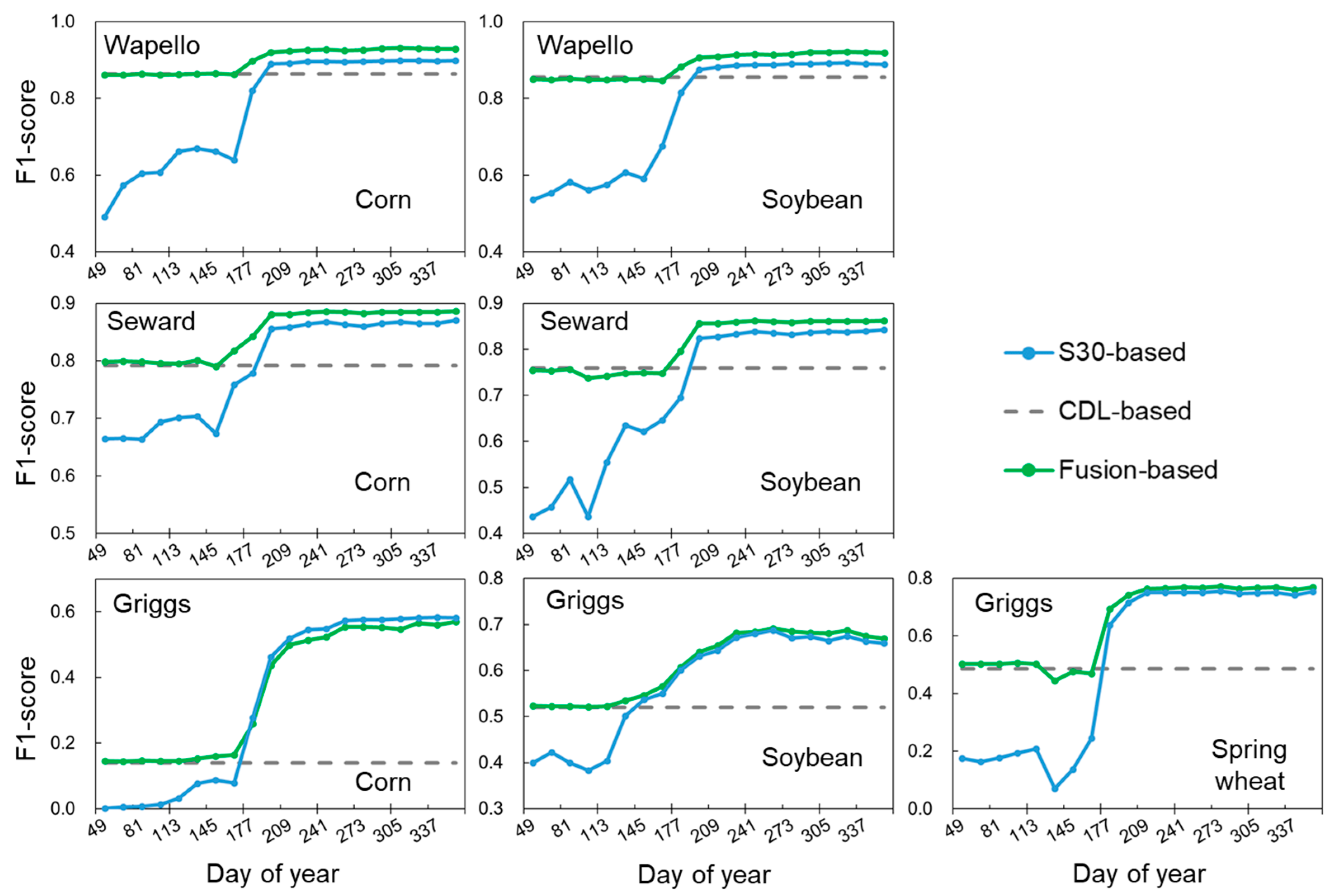
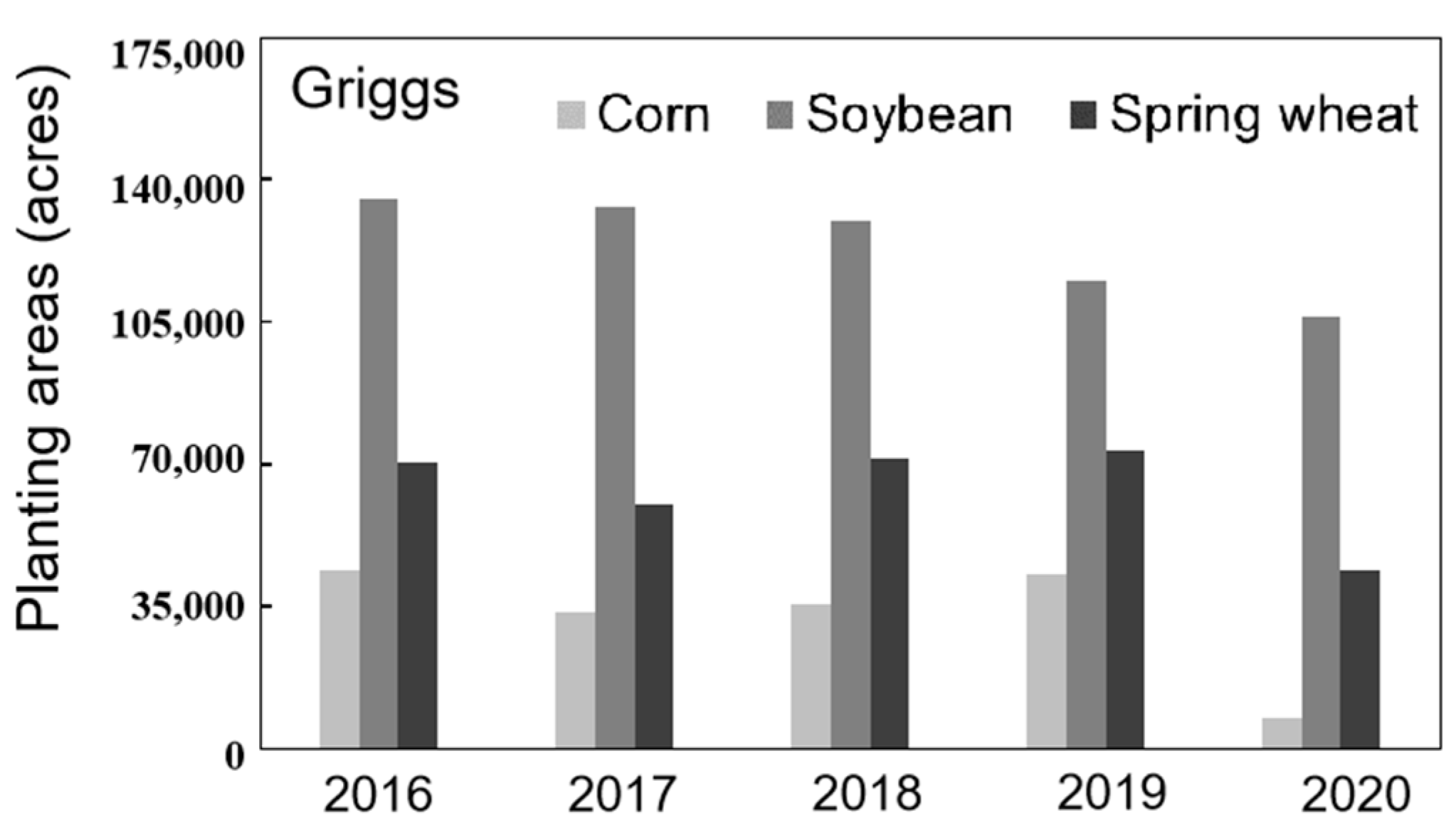
Figure 6 shows the performance of the main crop type identification using the S30 images. Combining the CDL-based with spectral-based classification generated a higher accuracy for corn and soybean identifications at the Wapello and Seward sites. For example, the fusion-based F1 score of corn reached above 0.85 at about 177 DOY at the two sites. For Griggs, the CDL-based, spectral-based, and fusion-based F1 scores showed similar change patterns as the other two sites; however, the CDL-based F1 scores of corn were much lower than that of soybean and spring wheat. We investigated the planting areas for different crop types from 2016 to 2020 in Griggs and found a substantial decrease in the corn planting area in 2020 (Figure 7), which may account for the CDL-based F1 scores of corn being less than 0.2.

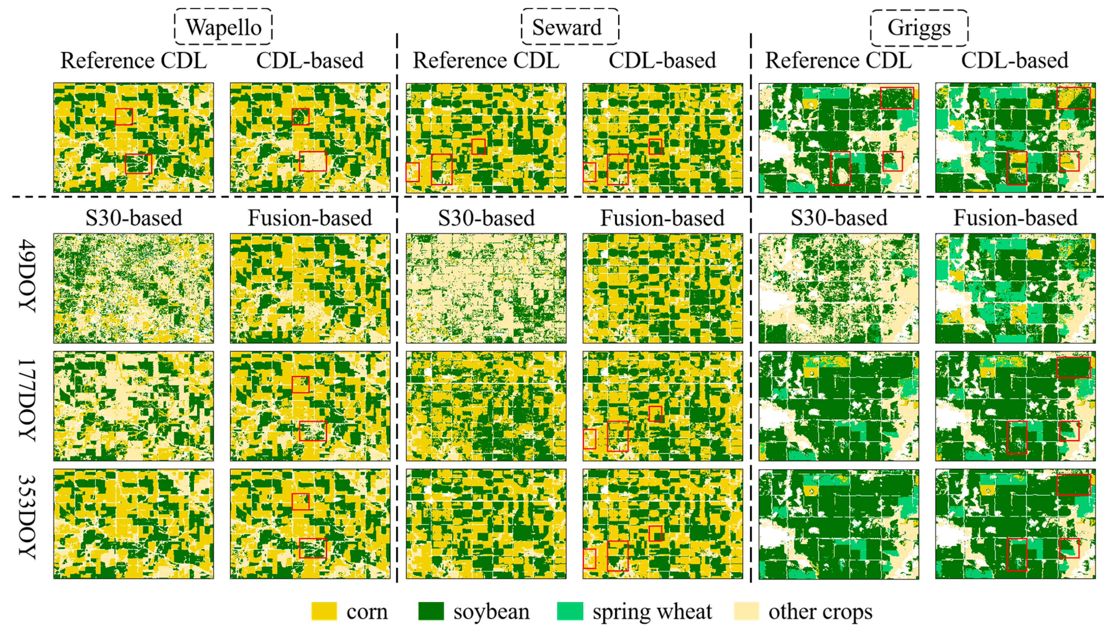
The comparisons between the crop classification maps and the reference CDL data are shown in Figure 8. Although the spatial patterns between the CDL-based classification and the reference maps are relatively consistent at the Wapello and Seward sites, the enlarged views of local areas show confusion errors among corn, soybean, and other crops (indicated by red boxes in Figure 8). With the inclusion of spectral information within the growing season, some crop fields with incorrect labels in the CDL-based classification were corrected in the fusion-based classification at 177 DOY (see the corresponding red boxes). More satisfactory results were obtained at the end of the year. In Griggs, consistent with the quantitative assessments, the CDL-based classification obviously overestimated the corn planting areas. This overestimation was corrected to some extent in the fusion-based classification as the growing season progressed.

3.2. Impact of Historical Crop Planting Pattern on Pre-Season Crop Classification

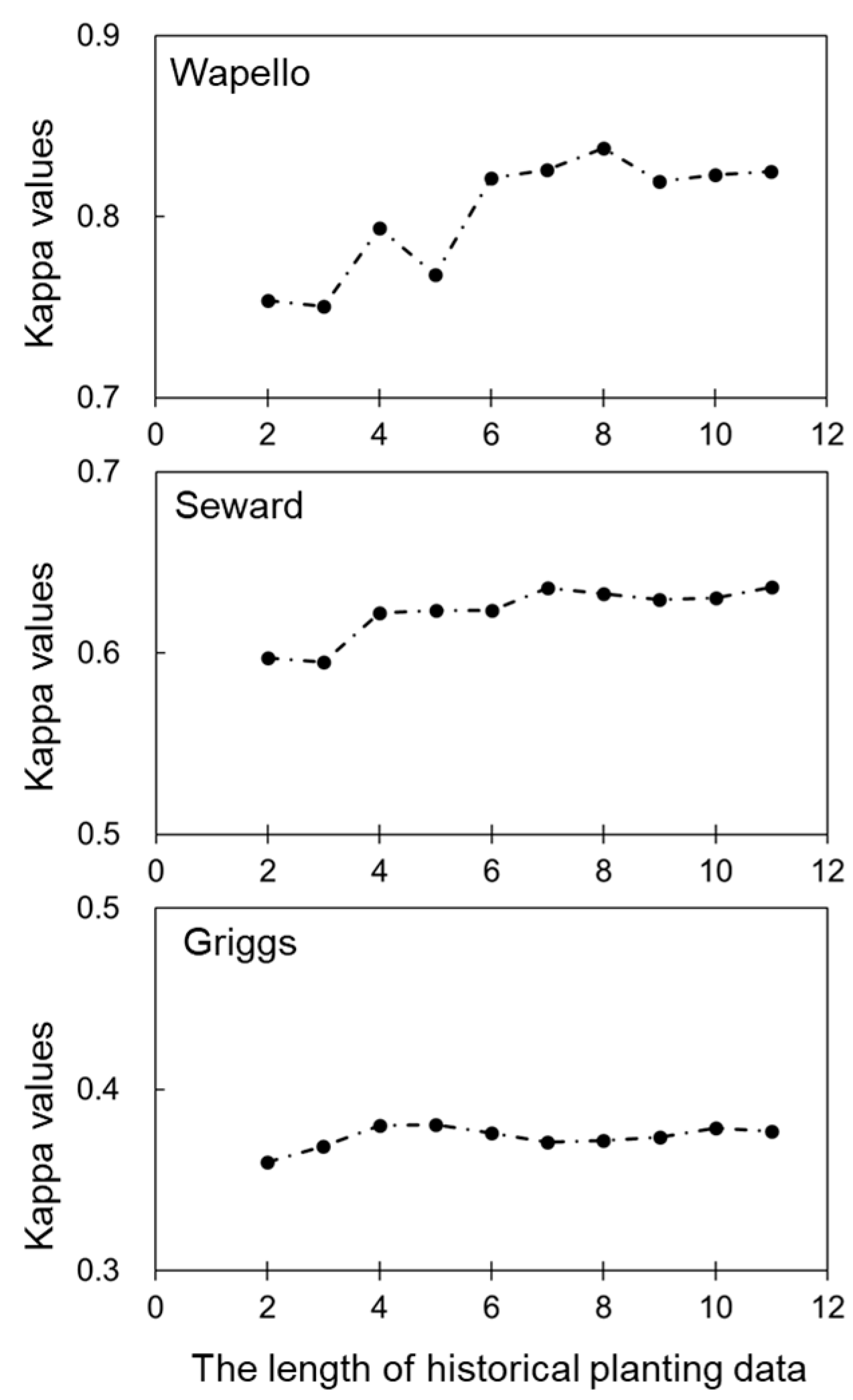
We first tested the performance of CDL-based crop classification using different numbers of years of CDL data prior to 2020. The results show that corn–soybean rotation patterns can be learned from approximately 5–6 years of historical CDL data, thus reaching a stable performance (Figure 9). We further used crop planting frequency as a surrogate to quantify crop rotation patterns. Specifically, we analyzed the number of times that corn and soybean were planted in the past 4, 6, 8, and 11 years before 2020. Pixels from the three sites were combined in this analysis. Both corn and soybean showed obviously better identification accuracy with two planting frequencies: continuous planting or planting in about half of the number of years (Figure 10). For example, higher F1 scores occur when identical crops were planted in 3 and 6 years in the past 6 years, and in 5–6 years and 9–11 years in the past 11 years.

3.3. Impact of Historical Crop Planting Data Errors on Crop Identification

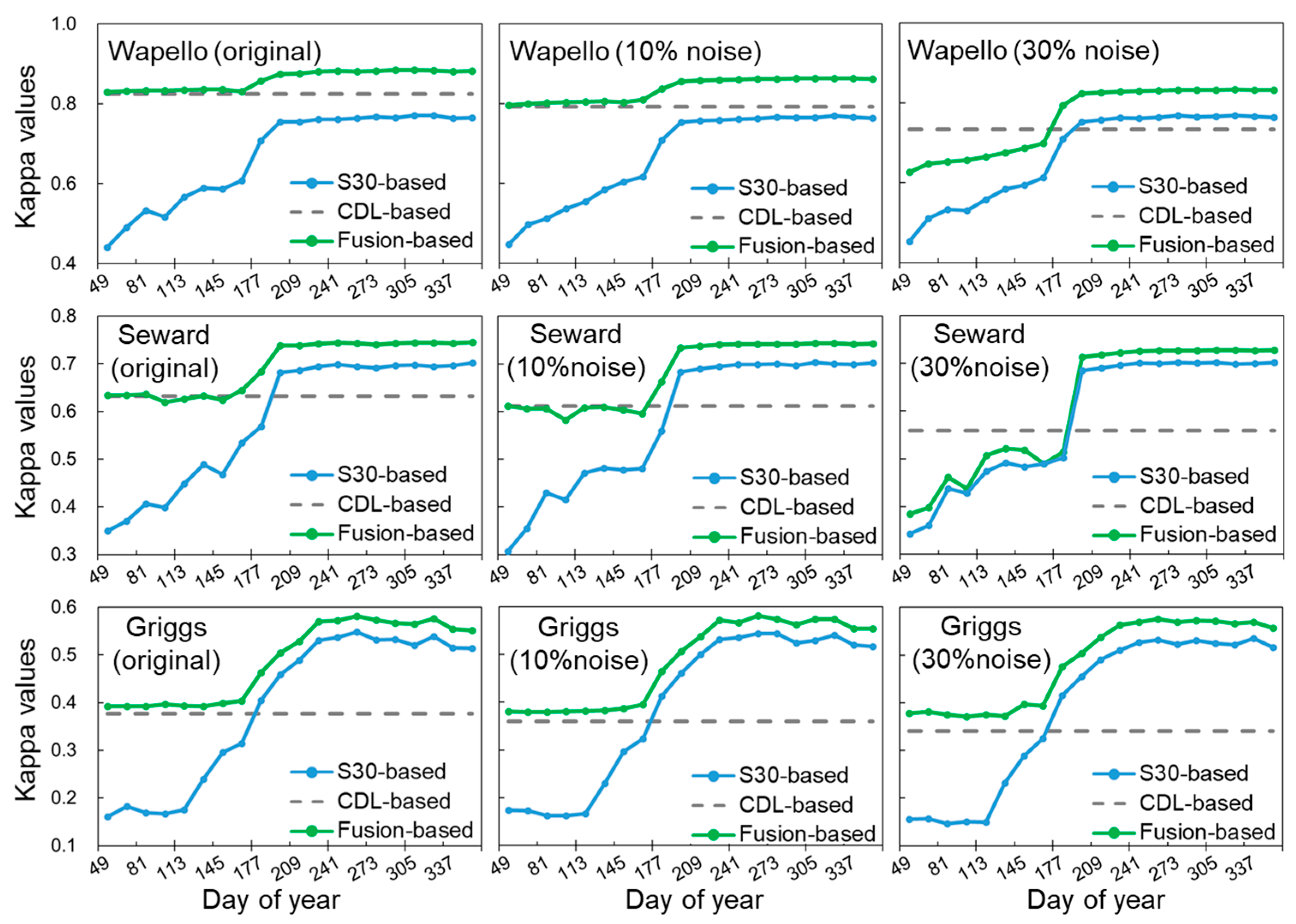
As reported in previous studies, the CDL data provided by USDA have a relatively high overall accuracy (85–95%) [35]. However, such CDL data were not released in many other countries of the world, implying that the historical planting data must be produced by individual users when applying the fusion method. Classification errors may be higher in these produced data. Therefore, we need to explore whether and to what extent the classification error of historical CDL data affects the performance of CDL-based, spectral-based, and fusion-based classifications. For this objective, we performed a simulation experiment by simulating classification errors in the historical CDL data at the three U.S. sites. To simulate different levels of classification errors, 10% (or 30%) pixels in the historical CDL dataset of each year were randomly labeled as the other crop types. For example, corn pixels in Wapello in a given year were mislabeled as soybean or other crops. The experimental results show that the CDL-based classification accuracy obviously decreased under the scenarios with simulated classification errors, whereas classification errors had less of an effect on the performance of spectral-based classification (Figure 11). In Wapello, the CDL-based Kappa values decreased from 0.83 to 0.80 (10% random error) and 0.74 (30% random error) and in Seward, the values decreased from 0.63 to 0.61 (10% random error) and 0.56 (30% random error). The decreases are smaller in Griggs due to the low CDL-based classification accuracy. The performance of fusion-based classification was also affected by simulated classification error, especially in the early periods. The soft classification probabilities of the CLD-based and spectral-based results are combined using the weights trained by the MLP module; thus, improper weights may be obtained using the training dataset with incorrect crop type labels, which accounts for the decreases in the fusion-based performance. This experiment highlights the necessity of high-quality historical crop planting data for pre- and within-season crop identification.

3.4. An Application of the Fusion Method at the Sichuan Site

We used the proposed fusion method to identify canola and winter wheat at the Sichuan site. Among the test samples in the year 2021, some were collected from ground investigations (354 samples) and others were collected from the visual interpretation of high-resolution images on Google Earth (385 samples). The results show that the change patterns of the CDL-based, spectral-based, and fusion-based accuracies at this site are similar to those observed at the three U.S. sites (Figure 12). The spectral-based F1 scores first increased as the growing season progressed and then exceeded the fixed CDL-based values. The fusion-based estimate incorporates the strengths of the CDL-based and spectral-based estimates and generated higher F1 scores throughout the growing season. Interestingly, we observed obvious differences for canola identification when using different test datasets for the evaluations (upper panels in Figure 12). The spectral-based F1 scores for canola based only on ground test samples are much smaller than the values evaluated with all test samples (0.73 vs. 0.84 at the end of the season), whereas the CDL-based F1 scores did not exhibit such differences between the two test datasets. These observations imply that there are obvious variations in canola identification accuracy across space, which may be attributed to the occurrence of cloud contamination during the flowering periods of canola at some locations. To verify this speculation, we calculated the Sentinel-2 image cloud coverage at the locations of the ground samples and visual interpretation samples. As we expected, there was an obviously higher cloud coverage for the locations of the ground samples during the important flowering periods (the range of the black dashed line in Figure S2), thus greatly decreasing the canola identification accuracy at these locations. For more accurate evaluations, it is necessary to collect more test samples under various conditions (e.g., variations in cloud coverage, crop phenology, and crop variety), although sample collection is time-consuming and labor-intensive.

4. Discussion

Crop types (e.g., corn and soybean) across the U.S. Corn Belt can be predicted from historical crop rotation patterns before the growing season [10]. As the growing season progresses, it is possible to perform the within-season crop identification for corn and soybean from time-series spectral information [5]. Inspired by the respective strengths of CDL-based and spectral-based crop classification, Johnson and Mueller (2021) proposed an innovative idea to integrate both CDL and spectral time-series data into a random forest model for within-season crop classification in the U.S. [32]. This study further clarified several important issues in the fusion of CDL-based and spectral-based crop classifications.

First, as one component of the fusion model, CDL-based crop classification is obviously more suitable for the areas with regular crop rotations (e.g., Wapello in Figure 9). However, how can we determine regular or irregular crop rotation patterns and their corresponding effect on the CDL-based classification? We found that the crop planting frequency in the past years may be a simple surrogate to estimate the CDL-based classification performance at the pixel level. A higher accuracy was observed for the pixels with either nearly continuous planting or half-time planting of the same crop (Figure 10). This finding may be explained by the common rotation patterns in the central U.S., such as the corn–soybean, corn–alfalfa, and soybean–spring wheat rotations [36]. At the testing site in Sichuan, historical planting data are also effective for the pre-season prediction of canola and winter wheat, with F1 scores above 0.7 (Figure 12). Although it is appealing to acquire a reasonable-looking predictive crop map at the beginning of year, this study found great uncertainties in the CDL-based predictions in two scenarios. One scenario is abnormal changes in crop planting structures. For example, although the planting conditions in the testing year 2020 were relatively normal across the U.S. Corn Belt, abnormal changes in crop planting areas still existed in some local areas, such as the Griggs site tested in this study, resulting in poor performance of CDL-based classification (Figure 9). In the abnormal year 2019 with heavy springtime precipitation in several states (e.g., Iowa and Illinois), corn planting was reported to be severely abandoned or the corn was switched with other crops [35]. It can be expected that crop distribution in 2019 cannot be reliably predicted from the historical CDL datasets. To quantify such an influence, we conducted an additional experiment to identify corn in Dekalb, a county located in Illinois, using 2018 and 2019 as the testing years. The results confirmed that the CDL-based F1 score for corn in 2019 decreased by about 10% compared with that in 2018 (Figure 13). Therefore, care should be taken for the CDL-based classification when weather anomalies occur or agricultural policy changes. The other scenario causing uncertainties in the CDL-based predictions is the use of archival land cover datasets with relatively serious classification errors. The experiment with simulated crop label errors suggests that high-quality historical crop planting data are particularly important for the CDL-based predictions, which greatly affect crop mapping at earlier times in the growing season (Figure 11). We need more crop distribution data with rigorous precision in countries outside of the U.S. [37].

Second, spectral-based crop classification is recognized as a good complement to pre-season predictions, providing very useful classification features particularly during the growth of corn and soybean through July [32]. Indeed, the F1 scores of corn and soybean for the spectral-based results exceeded those for the CDL-based predictions at the Wapello and Seward sites at the end of July (Figure 6). At the Griggs site, however, a similar pattern occurred one month earlier, owing to the less reliable CDL-based prediction. For the within-season spectral-based classification, we followed previous studies and did not used the within-season training data [5]. From a practical perspective, such a treatment is appealing given the difficulty in collecting training samples during the early growing season. Furthermore, the experiments also suggest the importance of consistency between training and testing data for spectral-based classification. The inconsistency in image cloud coverage between years substantially decreased the spectral-based classification performance (Figure 5). This influence may be particularly severe when some key spectral features are obscured, such as the canola flowering features at the Sichuan site due to higher cloud coverage during the flowering period in 2021 (Figure S2). Moreover, interannual variations in crop phenology also lead to inconsistencies between training and testing data. To improve the transferability of training data, time-series composited data with wider time windows (e.g., monthly composited) were suggested by previous studies. However, the wide-window composited strategy obviously decreases the timeliness of within-season crop classification. By integrating CDL-based prediction, the fusion-based classification was less sensitive to interannual inconsistencies and had a more stable performance at fine temporal scales (8-day).

Third, the proposed fusion method better incorporated the CDL-based and the spectral-based estimates compared to the random forest model adopted by Johnson and Mueller (2021). In the early periods of the growing season, we observed that the random forest model was greatly affected by the poor performance of spectral-based classification (Figure 3), which is consistent with the results in Johnson and Mueller (2021) (Figure 4 in their study) and may be explained as follows. The random forest classifier consists of many single decision trees. Each decision tree is trained by randomly selecting a given number of feature variables (m) from all feature variables (M; M > m) as well as a given number of samples from the entire training dataset. Each tree can generate a classification, i.e., we can say that the tree “votes” for that class. The forest normally determines the final classification as the one with the most votes from all trees [38]. Obviously, the ensemble learning strategy is unsuccessful when more than half of trees give an incorrect classification. This situation may be encountered in the early periods because more of the less useful spectral feature variables are selected by the trees, leading to the poor performance of each individual tree. Different from the feature fusion in the random forest model (i.e., at the feature-level), the proposed method directly fuses the CLD-based and spectral-based estimates (i.e., at the decision-level). The weights for the soft classification probabilities of the two estimates are determined by training an MLP module. The importance of spectral features varies as the growing season progresses and thus results in greater uncertainties in feature-level fusion, implying that the decision-level fusion strategy may be more suitable for within-season crop classification.

5. Conclusions

The challenge for within-season crop identification is the limited crop spectral information at early crop phenological stages. To address this issue, we proposed a deep learning-based fusion method to integrate the crop type estimates from crop spectral information with the estimates provided by crop rotation patterns. We aimed to answer the following three questions: (1) Is there a useful fusion method to generate reliable crop type estimates throughout the growing season? (2) What kinds of crop planting patterns are the most preferred for pre-season prediction? (3) How does classification errors in the historical crop planting data affect within-season crop identification? The experimental results showed that the crop planting patterns with either nearly continuous planting or half-time planting of the same crop can generate more accurate pre-season crop predictions. Moreover, pre-season crop predictions are greatly affected by the accuracy of the historical crop planting data. The crop classification results achieved by the proposed fusion method are comparable to the estimates based on crop rotation patterns in the early growing season and can be further improved as the growing season progresses because of the inclusion of more crop spectral information, thus producing reliable classification results throughout the entire growing season. Our study highlighted the great potential for real-time crop mapping through the fusion of spectral information and crop rotation patterns.

References

1. Gallego, J.; Carfagna, E.; Baruth, B. Accuracy, objectivity and efficiency of remote sensing for agricultural statistics. In Agricultural Survey Methods; Benedetti, R., Bee, M., Espa, G., Piersimoni, F., Eds.; John Wiley & Sons: Chichester, UK, 2010; pp. 193–211. [Google Scholar]
2. Konduri, V.S.; Kumar, J.; Hargrove, W.W.; Hoffman, F.M.; Ganguly, A.R. Mapping crops within the growing season across the United States. Remote Sens. Environ. 2020, 251, 112048. [Google Scholar] [CrossRef]
3. Boryan, C.; Yang, Z.; Mueller, R.; Craig, M. Monitoring US Agriculture: The US Department of Agriculture, National Agricultural Statistics Service, Cropland Data Layer Program. Geocarto Int. 2011, 26, 341–358. [Google Scholar] [CrossRef]
4. Mueller, R.; Harris, M. Reported uses of CropScape and the national cropland data layer program. In Proceedings of the International Conference on Agricultural Statistics VI, Rio de Janeiro, Brazil, 23–25 October 2013; pp. 23–25. [Google Scholar]
5. Cai, Y.P.; Guan, K.Y.; Peng, J.; Wang, S.W.; Seifert, C.; Wardlow, B.; Li, Z. A high-performance and in-season classification system of field-level crop types using time-series Landsat data and a machine learning approach. Remote Sens. Environ. 2018, 210, 35–47. [Google Scholar] [CrossRef]
6. Xiao, Y.; Mignolet, C.; Mari, J.; Benoît, M. Modeling the Spatial Distribution of Cropping Systems at a Large Regional Scale: A Case of Crop Sequence Patterns in France between 1992 and 2003. In Proceedings of the 12th Congress of the European Society for Agronomy, Helsinki, Finland, 20–24 August 2012. [Google Scholar]
7. Castellazzi, M.S.; Wood, G.A.; Burgess, P.J.; Morris, J.; Conrad, K.F.; Perry, J.N. A Systematic Representation of Crop Rotations. Agric. Syst. 2008, 97, 26–33. [Google Scholar] [CrossRef]
8. Le Ber, F.; Benoît, M.; Schott, C.; Mari, J.-F.; Mignolet, C. Studying Crop Sequences with CarrotAge, a HMM-Based Data Mining Software. Ecol. Model. 2006, 191, 170–185. [Google Scholar] [CrossRef]
9. Osman, J.; Inglada, J.; Dejoux, J.-F. Assessment of a Markov logic model of crop rotations for early crop mapping. Comput. Electron. Agric. 2015, 113, 234–243. [Google Scholar] [CrossRef]
10. Zhang, C.; Di, L.; Lin, L.; Guo, L. Machine-Learned Prediction of Annual Crop Planting in the U.S. Corn Belt Based on Historical Crop Planting Maps. Comput. Electron. Agric. 2019, 166, 104989. [Google Scholar] [CrossRef]
11. Yaramasu, R.; Bandaru, V.; Pnvr, K. Pre-season crop type mapping using deep neural networks. Comput. Electron. Agric. 2020, 176, 105664. [Google Scholar] [CrossRef]
12. Hu, F.; Xia, G.-S.; Hu, J.; Zhang, L. Transferring Deep Convolutional Neural Networks for the Scene Classification of High-Resolution Remote Sensing Imagery. Remote Sens. 2015, 7, 14680–14707. [Google Scholar] [CrossRef]
13. Hu, Q.; Wu, W.B.; Song, Q.; Yu, Q.Y.; Yang, P.; Tang, H.J. Recent Progresses in Research of Crop Patterns Mapping by Using Remote Sensing. Sci. Agric. Sin. 2015, 48, 1900–1914. [Google Scholar]
14. Qiu, B.; Luo, Y.; Tang, Z.; Chen, C.; Lu, D.; Huang, H.; Chen, Y.; Chen, N.; Xu, W. Winter Wheat Mapping Combining Variations before and after Estimated Heading Dates. ISPRS J. Photogramm. Remote Sens. 2017, 123, 35–46. [Google Scholar] [CrossRef]
15. Xiao, X.; Boles, S.; Liu, J.; Zhuang, D.; Frolking, S.; Li, C.; Salas, W.; Moore, B. Mapping paddy rice agriculture in southern Chinausing multi-temporal MODIS images. Remote Sens. Environ. 2005, 95, 480–492. [Google Scholar] [CrossRef]
16. Zang, Y.; Chen, X.; Chen, J.; Tian, Y.; Shi, Y.; Cao, X.; Cui, X. Remote Sensing Index for Mapping Canola Flowers Using MODIS Data. Remote Sens. 2020, 12, 3912. [Google Scholar] [CrossRef]
17. Sulik, J.J.; Long, D.S. Spectral indices for yellow canola flowers. Int. J. Remote Sens. 2015, 36, 2751–2765. [Google Scholar] [CrossRef]
18. Sulik, J.J.; Long, D.S. Spectral Considerations for Modeling Yield of Canola. Remote Sens. Environ. 2016, 184, 161–174. [Google Scholar] [CrossRef]
19. Tao, J.; Wu, W.; Liu, W.; Xu, M. Exploring the Spatio-Temporal Dynamics of Winter Rape on the Middle Reaches of Yangtze River Valley Using Time-Series MODIS Data. Sustainability 2020, 12, 466. [Google Scholar] [CrossRef]
20. Veloso, A.; Mermoz, S.; Bouvet, A.; Le Toan, T.; Planells, M.; Dejoux, J.F.; Ceschia, E. Understanding the temporal behavior of crops using Sentinel-1 and Sentinel-2-like data for agricultural applications. Remote Sens. Environ. 2017, 199, 415–426. [Google Scholar] [CrossRef]
21. Dong, J.; Xiao, X. Evolution of regional to global paddy rice mapping methods: A review. ISPRS J. Photogramm. Remote Sens. 2016, 119, 214–227. [Google Scholar] [CrossRef]
22. Clauss, K.; Ottinger, M.; Leinenkugel, P.; Kuenzer, C. Estimating Rice Production in the Mekong Delta, Vietnam, Utilizing TimeSeries of Sentinel-1 SAR Data. Int. J. Appl. Earth Obs. 2018, 73, 574–585. [Google Scholar]
23. Foerster, S.; Kaden, K.; Foerster, M.; Itzerott, S. Crop type mapping using spectral-temporal profiles and phenological information. Comput. Electron. Agric. 2012, 89, 30–40. [Google Scholar] [CrossRef]
24. Belgiu, M.; Csillik, O. Sentinel-2 cropland mapping using pixel-based and object- based time-weighted dynamic time warpinganalysis. Remote Sens. Environ. 2018, 204, 509–523. [Google Scholar] [CrossRef]
25. Dong, Q.; Chen, X.; Chen, J.; Zhang, C.; Liu, L.; Cao, X.; Zang, Y.; Zhu, X.; Cui, X. Mapping Winter Wheat in North China Using Sentinel 2A/B Data: A Method Based on Phenology-Time Weighted Dynamic Time Warping. Remote Sens. 2020, 12, 1274. [Google Scholar] [CrossRef]
26. Yi, Z.; Jia, L.; Chen, Q. Crop Classification Using Multi-Temporal Sentinel-2 Data in the Shiyang River Basin of China. Remote Sens. 2020, 12, 4052. [Google Scholar] [CrossRef]
27. Zhong, L.; Hu, L.; Zhou, H. Deep Learning Based Multi-Temporal Crop Classification. Remote Sens. Environ. 2019, 221, 430–443. [Google Scholar] [CrossRef]
28. Zhong, L.; Hu, L.; Zhou, H.; Tao, X. Deep learning based winter wheat mapping using statistical data as ground references in Kansas and northern Texas, US. Remote Sens. Environ. 2019, 233, 111411. [Google Scholar] [CrossRef]
29. You, N.; Dong, J. Examining earliest identifiable timing of crops using all available Sentinel 1/2 imagery and Google Earth Engine. ISPRS J. Photogramm. Remote Sens. 2020, 161, 109–123. [Google Scholar] [CrossRef]
30. Zaremba, W.; Sutskever, I.; Vinyals, O. Recurrent Neural Network Regularization. arXiv 2014, arXiv:1409.2329. [Google Scholar]
31. Xu, J.F.; Zhu, Y.; Zhong, R.H.; Lin, Z.X.; Xu, J.L.; Jiang, H.; Huang, J.F.; Li, H.F.; Lin, T. DeepCropMapping: A multi-temporal deeplearning approach with improved spatial generalizability for dynamic corn and soybean mapping. Remote Sens. Environ. 2020, 247, 111946. [Google Scholar] [CrossRef]
32. Johnson, D.M.; Mueller, R. Pre- and within-Season Crop Type Classification Trained with Archival Land Cover Information. Remote Sens. Environ. 2021, 264, 112576. [Google Scholar] [CrossRef]
33. Zhou, P.; Shi, W.; Tian, J.; Qi, Z.; Li, B.; Hao, H.; Xu, B. Attention-based bidirectional long short-term memory networks forrelation classification. In Proceedings of the 54th Annual Meeting of the Association for Computational Linguistics (Volume 2: Short Papers), Berlin/Heidelberg, Germany, 7–12 August 2016; pp. 207–212. [Google Scholar]
34. Claverie, M.; Ju, J.; Masek, J.G.; Dungan, J.L.; Vermote, E.F.; Roger, J.-C.; Skakun, S.V.; Justice, C. The Harmonized Landsat andSentinel-2 Surface Reflectance Data Set. Remote Sens. Environ. 2018, 219, 145–161. [Google Scholar] [CrossRef]
35. Gao, F.; Zhang, X. Mapping Crop Phenology in Near Real-Time Using Satellite Remote Sensing: Challenges and Opportunities. J. Remote Sens. 2021, 2021, 8379391. [Google Scholar] [CrossRef]
36. USDA; National Agricultural Statistics Service. Field Crop Usual Planting and Harvesting Dates; NASS: Washington, DC, USA, 2010. [Google Scholar]
37. Han, J.; Zhang, Z.; Luo, Y.; Cao, J.; Zhang, L.; Zhang, J.; Li, Z. The RapeseedMap10 database: Annual maps of rapeseed at a spatial resolution of 10 m based on multi-source data. Earth Syst. Sci. Data 2021, 13, 2857–2874. [Google Scholar] [CrossRef]
38. Breiman, L. Random forests. Mach. Learn. 2001, 45, 5–32. [Google Scholar] [CrossRef]
Figure 1. The neural network structure of the proposed within-season crop identification model.
Remotesensing 15 05043 g001
Figure 2. The fusion of spectral time-series data and historical planting data for within-season crop mapping was evaluated in three counties in the U.S. (left) and one cloudy region in Sichuan Province in southwest China (right). At the Sichuan site, we show the spatial distribution of all testing samples generated by both ground collection and visual interpretation.
Remotesensing 15 05043 g002
Figure 3. The performance of crop classification using the proposed fusion method (left) and the random forest model (right) at the three U.S. sites. In each panel, we show the kappa values for the CDL-based, spectral-based (L30, S30, or HLS), and the fusion-based crop classifications as the growing season progresses.
Remotesensing 15 05043 g003
Figure 4. The cloud coverage (mean and standard deviation) in the L30 and S30 images acquired during the period (145–193 DOY) at the Seward site in each year.
Remotesensing 15 05043 g004
Figure 5. The performance of spectral-based (L30 or S30) crop classification at the Seward site using the data from different years as the training data.
Remotesensing 15 05043 g005
Figure 6. The performance of proposed fusion method in main crop type identification at the three U.S. sites. Each panel shows the F1 scores for the CDL-based, S30-based, and the fusion-based results throughout the crop season.
Remotesensing 15 05043 g006
Figure 7. The planting areas of corn, soybean, and spring wheat at the Griggs site in each year.
Remotesensing 15 05043 g007
Figure 8. The comparison between the 2020 U.S. crop classification maps and the reference CDL data. The red frames in panels highlight the differences between classification results and reference data. The dashed lines are included to separate each testing region to help visual inspection.
Remotesensing 15 05043 g008
Figure 9. The performance of CDL-based crop classification (Kappa values) using different numbers of years of historical planting data at the three U.S. sites.
Remotesensing 15 05043 g009
Figure 10. The relationship between crop planting frequency and crop classification performance. Here, crop planting frequency is calculated as the number of times (e.g., 1–4 in the first panel) corn (or soybean) were planted in the past (e.g., four years in the first panel).
Remotesensing 15 05043 g010
Figure 11. The performance of crop classification through the crop season under different scenarios with simulated different levels of error (10% and 30%) in the historical CDL datasets.
Remotesensing 15 05043 g011
Figure 12. The performance values of canola and winter wheat identifications throughout the crop season at the Sichuan site. The F1 scores are calculated using only the samples collected on the ground (right panels) or using both the ground samples and the samples collected from the visual interpretation of high-resolution images on Google Earth (left panels).
Remotesensing 15 05043 g012
Figure 13. The performance of CDL-based, S30-based, and fusion-based classifications for corn in the Dekalb County (located in Illinois) using the years 2018 and 2019 as the testing data.
Remotesensing 15 05043 g013