HFCC-Net: A Dual-Branch Hybrid Framework of CNN and CapsNet for Land-Use Scene Classification

Abstract

Land-use scene classification (LUSC) is a key technique in the field of remote sensing imagery (RSI) interpretation. A convolutional neural network (CNN) is widely used for its ability to autonomously and efficiently extract deep semantic feature maps (DSFMs) from large-scale RSI data. However, CNNs cannot accurately extract the rich spatial structure information of RSI, and the key information of RSI is easily lost due to many pooling layers, so it is difficult to ensure the information integrity of the spatial structure feature maps (SSFMs) and DSFMs of RSI with CNNs only for LUSC, which can easily affect the classification performance. To fully utilize the SSFMs and make up for the insufficiency of CNN in capturing the relationship information between the land-use objects of RSI, while reducing the loss of important information, we propose an effective dual-branch hybrid framework, HFCC-Net, for the LUSC task. The CNN in the upper branch extracts multi-scale DSFMs of the same scene using transfer learning techniques; the graph routing-based CapsNet in the lower branch is used to obtain SSFMs from DSFMs in different scales, and element-by-element summation achieves enhanced representations of SSFMs; a newly designed function is used to fuse the top-level DSFMs with SSFMs to generate discriminant feature maps (DFMs); and, finally, the DFMs are fed into classifier. We conducted sufficient experiments using HFCC-Net on four public datasets. The results show that our method has better classification performance compared to some existing CNN-based state-of-the-art methods.

1. Introduction

As remote sensing technology continues to develop, LUSC plays an increasingly important role in the field of remote sensing [1]. For instance, the support of LUSC is needed in the fields of ecological environment construction, urban construction planning, disaster analysis, and disaster relief resource dispatching [2,3]. Most importantly, with the continuous improvement of the decision-making system and management level in various fields of the country, people’s needs and requirements for surface target information are becoming higher and higher, and the technology of LUSC has inevitably become a key technical subject of wide concern in the field of remote sensing [4,5].

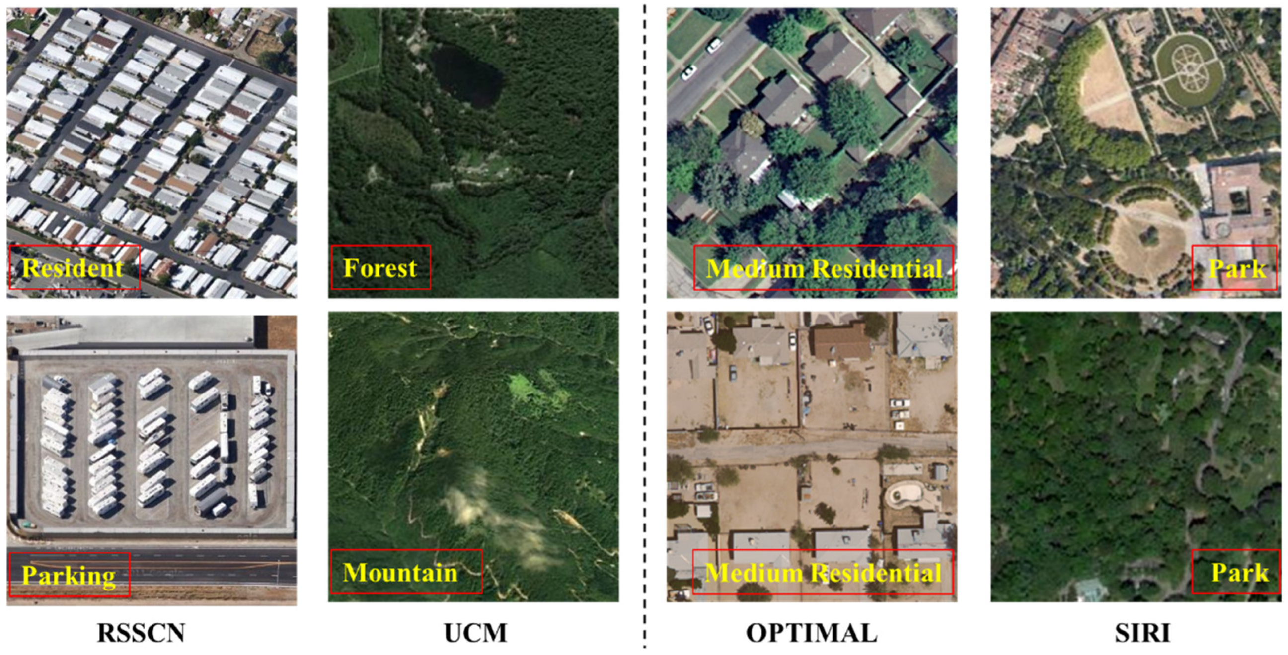
In land-use scene images (LUSIs), there is a large difference between images of the same category and a high degree of similarity between images of different categories. As shown in Figure 1, the semantic expressions of images in the categories of “Resident” and “Parking” in the RSSCN7 dataset have a high degree of similarity, and those of “Forest” and “Mountain” in the UCM dataset do; moreover, the semantic expressions of images in the categories of “Medium Residential” in the OPTIMAL dataset and “Park” in the SIRI dataset have a high degree of difference. In addition, affected by the diversity, multi-resolution, and complex spatial content distribution of LUSIs, the LUSC task of automation and high accuracy is, subsequently, full of uncertainties. Therefore, it has become a challenging task to adequately express the detailed features of different land-use category images and achieve high accuracy classification results.

The traditional technique is to use manual design of features [6]. One class is pixel-based classification: each pixel is considered as the smallest classification unit, and the spectral, morphological, textural, and spatial information of the pixel is first extracted, from which the features that can represent the different classes are then selected and classified using different classifiers. This type of approach is susceptible to image local heterogeneity and noise in high-resolution images [7]. The other category is object-based classification: segmentation based on a specific target in the image and its spatial structural relationship, combining multiple pixel points into an object with similar features, so as to achieve the purpose of feature extraction, analysis, and classification. In such methods, the classification results are limited by the goodness of the segmentation results [8]. Moreover, traditional techniques need to rely on experts’ empirical analyses and a lot of manually designed features, which are not only time-consuming and labor-intensive, but also easy to fall into local extremes [9]. These characteristics lead to the fact that when using traditional methods to deal with the task of classifying a large number of LUSIs based on RSI data, not only is the efficiency of the classification is not high, but also the accuracy of the classification cannot be stable all the time.

The latest techniques for LUSC are based on deep learning methods, which automatically learn image features with multiple characteristics through the network, and use a large number of labeled samples to quickly fit an image classification model [10]. Owing to the ability to automatically learn image features and the high classification accuracy, CNN-based methods have become the most popular methods for LUSC. First, a convolutional layer is used to filter the input image with multiple channels to capture information such as different textures, shapes, and colors in the image; second, the pooling layer is used to reduce the size and computation of the feature map and improve the computational efficiency; and last, the fully connected layer is used to map the features output from the pooling layer to the corresponding category labels to achieve the goal of LUSC. To prevent overfitting and improve the generalization ability of the model, the method often employs some regularization techniques such as dropout and batch normalization, which can help reduce the number of parameters in the network, improve the robustness of the model, and make the network easier to train and optimize. However, during the process of pooling RSIs, not only is a lot of effective information lost, but also the spatial resolution of the image is reduced; moreover, the noise on the image and the effect of image rotation and scaling due to the change of viewpoints have a relatively large impact on the accuracy of target category interpretation. All these are also major issues that affect the further development of CNN-based techniques in LUSC [11].

CapsNet was proposed by Hinton et al. in 2017 [12], and was mainly proposed to address the limitations of traditional CNNs in tasks such as pose estimation, and its core idea is to replace neurons in traditional neural networks with capsules, and to capture spatial relationships and hierarchical structures between objects by introducing dynamic routing algorithms, so as to improve the robustness and generalization ability of the model. In recent years, it has been successfully applied to tasks such as brain tumor image classification [13], gait recognition [14], iris recognition [15], and LUSC [16], with good results. Compared with CNN-based classification methods, CapsNet-based methods are more expressive in feature extraction and representation of images, which is manifested in three aspects: 1. Pose invariance: it can better learn and express the pose information in the input data, which enables it to have a significant advantage in recognizing objects with different poses; 2. Hierarchical representation: features are represented as vectors in the capsule through a dynamic routing algorithm, and this hierarchical representation can better capture the spatial relationship and contextual information between features; 3. Robustness: with a certain degree of robustness, it can better cope with the problems of noise, deformation, and interference in the input data [17]. Although CapsNets have shown potential advantages in a number of tasks, some shortcomings still exist at present. For example, the introduction of a large number of dynamic routing operations has led to an increase in the complexity of the network and slower training and inference, and the current architecture is still relatively simple, which needs to be further optimized and improved to accommodate larger image data [18].

For the purpose of further improving the classification accuracy of LUSIs, especially for RSIs with relatively high image resolution, large heterogeneity of image content, and certain noise, features extraction and interpretation ability of commonly used network models on LUSIs need to be further improved, which requires the use of the spatial structure information of RSIs in the meantime, and, thus, reduces the loss of important feature maps in the process of DSFM extraction and the issue of category misclassification during scene classification. Therefore, we propose to design a novel scene classification model, called HFCC-Net, which combines the strengths of image object location and pose perception based on the CapsNet approach together with the advantages of DSFM extraction capability of the CNN-based method, to provide richer feature representations and more accurate scene category determination results for the LUSC task. The main contributions are as follows:

• We designed a novel LUSC method named HFCC-Net with hybrid CapsNet and CNN, which could fully utilize the global semantic information and local spatial structure information of RSIs to effectively represent global and local feature maps, and obtained competitive level of classification compared with the advanced ones;
• We propose an algorithm for generating discriminative feature maps, which could fuse the global DSFMs obtained through CNN and the local SSFMs obtained by the graph routing-based CapsNet, and not only achieves the maximization of the information content for feature representation, but also improves the classification accuracy;
• We conducted full experiments on four typical LUSI datasets, and not only successfully verified the advancement of HFCC-Net, but also analyzed in detail the main factors affecting the classification accuracy.

The rest of the paper is organized as follows: in Section 2, a description of the relevant studies is given; Section 3 presents the data and evaluation indicators; Section 4 discusses the proposed methodology; Section 5 conducts experiments and discusses the factors influencing; and finally, conclusions are drawn in Section 6.

2. Related Work

2.1. CapsNet-Based for Classification

In recent years, researchers have conducted extensive research and in-depth exploration of CapsNet-based image classification techniques, and the related results are mainly reflected in three aspects. First, the routing algorithm is improved. Sabour et al. [12] proposed an adaptive routing algorithm, which regards the number of routing times as the hyper-parameters of the model and dynamically adjusts the number of routing times according to the performance in the training process, so that the model can better learn the distributional characteristics of the data and improve the classification accuracy. Hinton et al. [19] use a 4 × 4 matrix to express the pose parameters of the object and switch to an expectation–maximization routing algorithm, which reduces the transformation matrix and reduces the training parameters and computational effort. Li et al. [20] treat the capsules in each layer as nodes of a graph and use bidirectional graph routing to learn the internal relationships between capsules in the same layer. Second, the architectural design of capsule network is improved. Tao et al. [21] propose using an adaptive capsule layer instead of the main capsule layer of CapsNet, thus, effectively utilizing the potential spatial relationships between capsule vectors and, thus, improving the classification accuracy. Phaye et al. [22] designed a dense CapsNet using dense layers instead of convolutional layers, and a diverse CapsNet using a hierarchical architecture to learn capsules, both with improved model performance. Xiong et al. [23] added a convolutional capsule layer and a capsule pooling layer to the original network, which reduced the number of model parameters and improved the experimental efficiency. Jia et al. [24] constructed multi-scale master capsules using residual convolutional layers and positional dot products, and used a sigmoid function to determine the weight coefficients between capsules, achieving better recognition performance. Zhou et al. [25] utilize twin capsule networks to solve the problem of information loss in the processing of remote sensing images by convolutional networks. Third, capsule attention mechanism is introduced. Hoogi et al. [26] added a capsule attention mechanism, which can adaptively focus on the important features in the image, enhance the important capsule at the same time, can inhibit the influence of irrelevant capsule, and improve the accuracy of the model. Gu et al. [27] replace the original dynamic routing method with an image pooling approach using multiple heads of attention, which not only makes the model computationally smaller, but also has better classification performance and adversarial robustness. Yu et al. [28] add an attention module for channel and spatial feature calibration, which results in higher quality target features learned by the network, sharper semantic information, and further improvement in the final classification accuracy. Although the above methods are able to achieve an improvement in image classification efficiency and accuracy, these methods are basically applied to image datasets with small samples, and have not been attempted in LUSI datasets. Furthermore, the architecture of CapsNet is still relatively simple, which makes it difficult to achieve better results in the classification of higher resolution and larger size RSIs for the time being.

2.2. CNN-Based for Classification

Among the latest scene classification approaches, CNN has become a classical neural network for processing image structured data. According to the means of classification feature map extraction, CNN-based classification methods can be classified into two categories: pure convolutional classification methods and classification methods in which convolution is fused with other different networks. For example, Xia et al. [29] processed RSI data using VGG network, GoogLeNet network, and AlexNet network, and achieved a high classification accuracy with the participation of pre-trained models. Sun et al. [30] fuse the DSFMs extracted from different convolutional layers of VGG-16 and select the best combination, which realizes the full utilization of complementary information between multi-layer DSFMs. Yu et al. [31] utilize two CNN networks to extract the original image and significantly enhanced image, respectively, and finally the two feature maps are fused for classification. Zhang et al. [32] enhance the model classification rate by adding channels and spatial attention to MobileNet V2. Yang et al. [33] propose the use of twinned CNNs for scene classification. Anwer et al. [34] propose using the ResNet network to extract the RGB features and texture encoding features of the model, and realize feature fusion by constructing a two-branch feature extraction architecture, and then achieve the effect of classification. Gao et al. [35] augmented the DSFMs extracted by CNN using the attention mechanism in the channel and spatial branches, and used the augmented fused features for scene classification. Liu et al. [36] improve classification performance by fusing different layers of feature maps from a single CNN. Wu et al. [37] build on the research of CNNs and propose stacking multiple columns of encoders for classification. Although methods such as combining different DSFMs or increasing the attention mechanism can reach a high scene classification accuracy, they do not solve the loss of information problem in the process of RSI feature map learning. In addition, researchers have proposed fusing CNN with other different networks in the hope of achieving complementary use of the strengths of different networks. For instance, Wang et al. [38] combine CNN and LSTM and add the attention mechanism, which speeds up the convergence and improves the accuracy. Zhang et al. [16] utilize VGG-16 and Inception-v3 in tandem with CapsNet to form a new network for classification, and achieve some results, but the convolutional network at the front of the whole network is still lossy, resulting in insufficient classification accuracy. Peng et al. [39] combine GNN and CNN to construct the spatial and topological relations of RSIs, and the classification accuracy reaches an advanced level. Obviously, this type of method can achieve higher classification accuracy, but it also increases the computational amount of feature learning, and in addition to the complexity of the combined model being higher, more importantly, it does not solve the loss messages of the feature maps and classification errors existing in the CNN itself.

2.3. Fusions for Classification

Along with the continuous in-depth study of the LUSC task, researchers began to try to use CapsNet to make up for the shortcomings of CNN-based techniques in the image classification task, and gradually achieved better classification results. Divided according to the manner in which these two network frameworks are combined, this fusion scene classification method can be divided into two types: one is fusion in the form of a sequence. The CNN first performs feature extraction on the input image and then feeds the extracted features into CapsNet for further processing. This approach allows the model to capture more complex patterns with CapsNet on top of the CNN. For example, Xu et al. [14] implement a network framework for gait image recognition by connecting convolutional and capsule modules in series. Phaye et al. [40] combine DenseNet and CapsNets to formulate better master capsules, creating an efficient recognition framework. Xiang et al. [41] use CFMs of different scales as inputs to the CapsNet to learn features and obtain a rich representation to achieve high recognition accuracy. Jampour et al. [42] use the deep features extracted from the second residual block of ResNet as the input data to CapsNet to obtain recognition results. Wang et al. [43] use ResNet to extract LiDAR data features and then use CapsNet for recognition, which solves the problem of information loss in ResNet network to some extent. Yousra et al. [44] extract features from the VGG19 model trained on the ImageNet dataset and input them into the newly designed CapsNet to obtain recognition results. In contrast to the above approach, Zhang et al. [45] input the features acquired through the CapsNet into MobileNetV2, which achieves the lightweight and accurate recognition requirements. This method is still based on CapsNet in essence, the difference is that the original input image data are replaced by the DSFM after the convolution operation; although it achieves certain image classification requirements, in the process of convolution of the image, part of the information is also lost. Another is fusion in a parallel form. The CNN and CapsNet are connected in parallel and each processes the input image and then the respective outputs are merged and classified. This approach can simultaneously utilize the excellent feature extraction capabilities of CNN and the powerful structure-aware capabilities of CapsNet. For example, Wang et al. [46] design a dual-channel network framework that fuses CNN and CapsNet, extracts convolutional and capsule features simultaneously and separately for the input data, then fuses the two features to form new classification features with more discriminative information, and finally inputs the fused features into a classifier to achieve classification. This type of method utilizes only single-scale DSFMs of the input image for the feature learning process in the CapsNet branch, and the two-branch feature fusion approach is simple and prone to produce redundant features and, furthermore, there is no improvement to CapsNet and CNN.

3. Materials

3.1. LUSI Datasets for LUSC

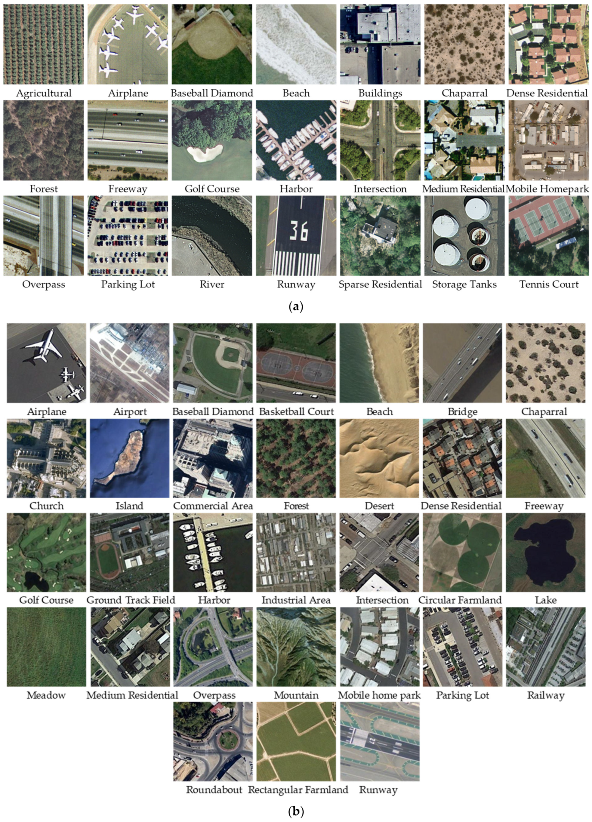
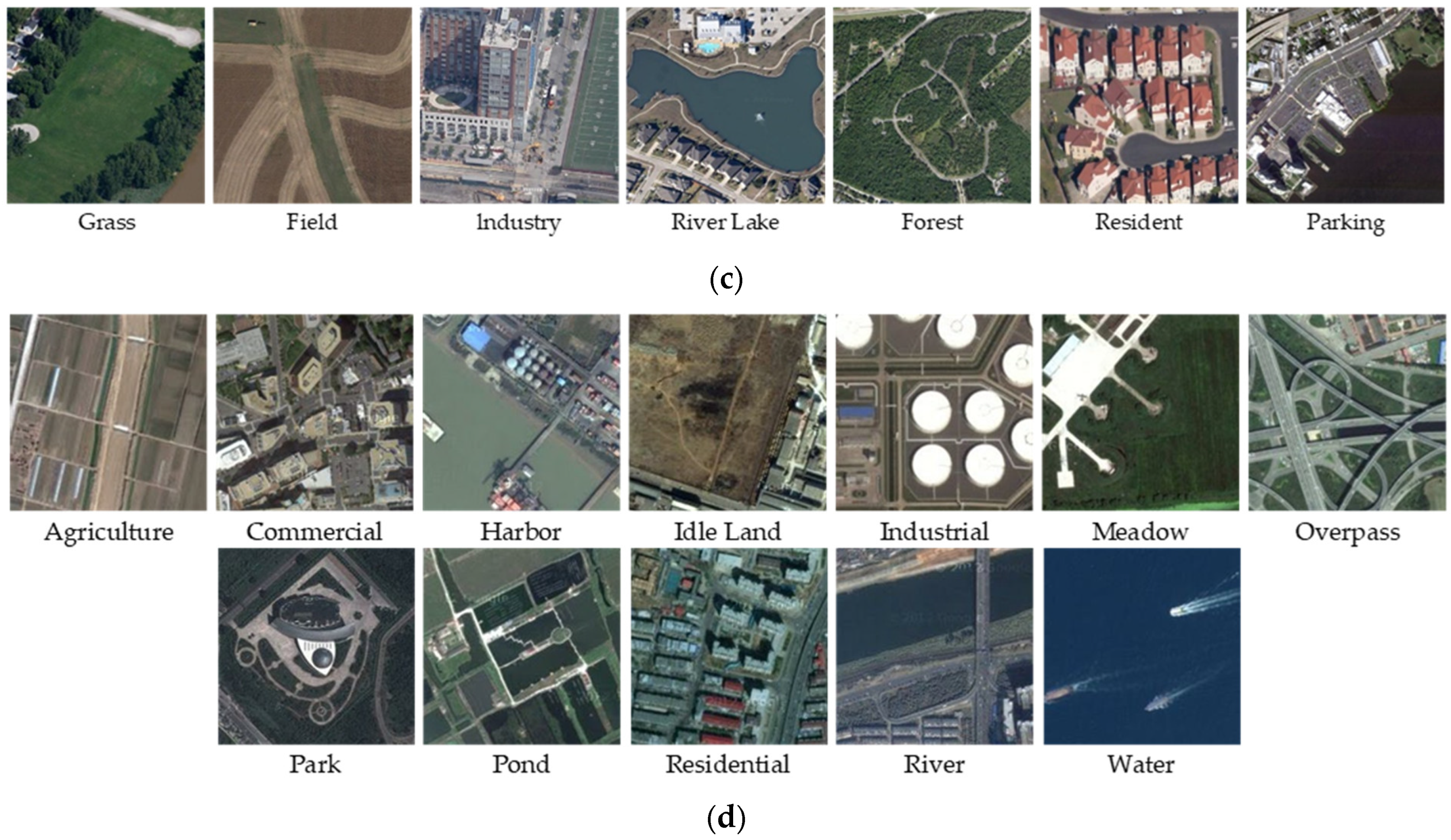
We used four typical LUSI datasets to conduct experiments and validate our proposed algorithm about scene classification. The specific parameters of the datasets are shown in

Table 1. Relevant parameters of the LUSI datasets.

Land Use Datasets	RSSCN	SIRI	UCM	OPTIMAL
Category number	7	12	21	31
Number per category	400	200	100	60
Total number	2800	2400	2100	1860
Image size	256 × 256	200 × 200	256 × 256	256 × 256
Source	Google Earth	GF-1 et al.	USGS	Google Earth

, and Figure 2 illustrates the samples for each land-use category.

(1) RSSCN [47]: The dataset contains images from seven different scenes with high spatial resolution, and the images of each scene come from different viewpoints, lighting conditions, and seasonal variations, which not only provide more detailed information about the features, but also simulate the real RSI scenes;

(2) SIRI [48]: The dataset is organized from data acquired by satellite sensors such as GF-1 and GF-2, as well as a number of global and domestic open datasets. These images cover images from different geographic locations, light conditions and seasons, including farmland, forests, cities, etc., which can provide diversity and richness of scene types and help to carry out refined RSI processing and analysis;

(3) UCM [49]: The dataset provides images with high spatial resolution, which can provide more detailed and clear RSI information, which is very important for conducting refined RSI processing and analysis. Moreover, both the categories of geographic scenes and the size of the dataset satisfy the need to utilize experiments to validate the algorithms;

(4) OPTIMAL [38]: The dataset is a multimodal RSI dataset that contains many types of remote sensing data, such as optical, radar and infrared images. This enables the dataset to reflect the diversity and richness of RSI data more comprehensively. In addition, the images in it not only cover rich geographic scenes, but also have a high data scale.

3.2. Evaluation Metrics for LUSC

(1) Scene classification accuracy (SCA): It is an intuitive evaluation metric, which is a benchmark for comparing the performance of different classification algorithms or different datasets, and can directly tell us how well the algorithms classify the whole dataset. Assuming that land-use category of ${\mathit{scene}}_i$ in the categorized dataset is ${\mathit{prediciton}}_i$, land-use category kind is $(0,1,2,\cdot \cdot \cdot ,j)$, and the function to predict the category of LUSI is $f$, the $SCA$ is calculated as follows:

$$SCA=\frac{{\displaystyle \sum _{i=0}^{j+1}(f(scen{e}_i)=predictio{n}_i)}}{j+1}$$

(1)

(2) Confusion matrix (CM): It can reflect the mutual misclassification probability between images of various categories. Formally, it is a two-dimensional matrix, with rows and columns representing the true and predicted labels of the images, respectively, and the values of the elements on the diagonal lines indicate the probability that the samples of the corresponding categories are correctly classified, while the values of the elements on the off-diagonal lines indicate the probability that the samples with the true labels are misclassified.

Shown in

Table 2. Schematic representation of the CM.

Probability Value		True Category Labels
		${\mathit{scene}}_0$	${\mathit{scene}}_1$	$\dots$	${\mathit{scene}}_{\mathit{j}}$	${\mathit{scene}}_{\mathit{j}+1}$
Predicted Category Labels	${\mathit{scene}}_0$	1	0	0	0	0
	${\mathit{scene}}_1$	0	1	0	0	0
	$\dots$	0	0	1	0	0
	${\mathit{scene}}_j$	0	0	0	1	0
	${\mathit{scene}}_{j+1}$	0	0	0	0	1

, for a scene classification task containing $j$ categories, the CM is a $j\times j$ matrix, where the $i$-th row and $j$-th column denote the probability that a target of category $i$ is classified into category $j$. We show the CM obtained by the best classifier, and, as can be seen, the probability values on the diagonal line are the largest.

4. Methodology

4.1. Overall Framework of HFCC-Net

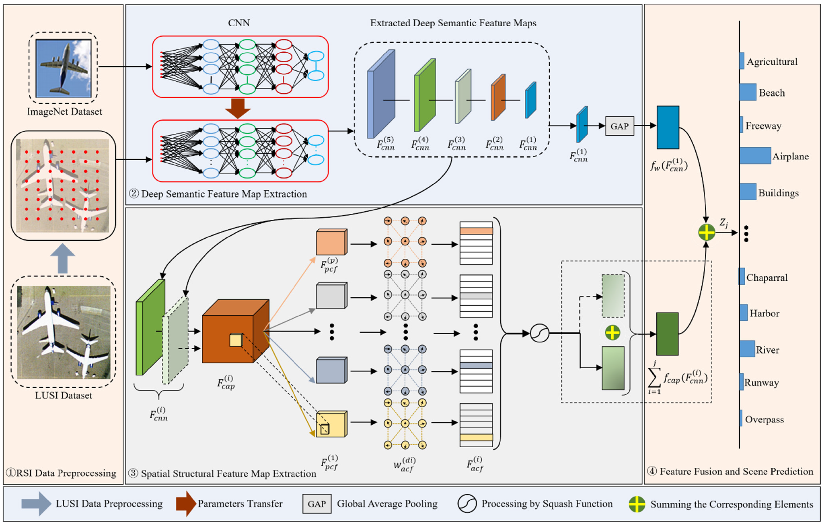
HFCC-Net is a novel scene classifier with a two-branch network architecture (see Figure 3), which can classify the deep semantic and spatial structure features extracted by CNN and CapsNet at the same time after fusion, and has an outstanding performance in dealing with LUSC with complex background contents. The overall structure of HFCC-Net consists of three parts: the DSFM extraction branch built by the transfer-learning-based CNN, the SSFM extraction branch built by the graph routing-based CapsNet, and the DFM and prediction module generated by fusing the two branches.

Before inputting the RSI data into the network, the data are first processed to be classified by the model. That is, it mainly consists of three steps: the first step is to crop the image to match the input size of the model (we set the size of the image as 224 × 224); the second step is to decode the image data into tensor data; and the third step is to convert the pixel values into floating point data type and perform normalization.

In HFCC-Net, considering that the training cost of utilizing CapsNet is higher than utilizing CNN, for example, utilizing CapsNet requires more computational resources and training time when dealing with a large number of high-resolution RSIs, in order to achieve the task of model training faster and more accurately, instead of choosing to utilize the original image data directly for the computation, we chose to use the DSFMs extracted by CNNs in the upper branch as the input data to the lower branch of the CapsNet. Inspired by the literature [27], we integrated the graph structure into the CapsNet in the lower branch, and utilized the multi-head attention graph-based pooling operation to replace the routing operation of the traditional method, which further reduced the training volume of HFCC-Net. Meanwhile, we utilized a transfer learning technique in computing DSFM, using pre-trained models from the ImageNet dataset.

In addition, we designed a new feature fusion algorithm to generate the DFM for improving the utilization efficiency of DSFM and SSFM. Finally, the DFM was fed into the classifier consisting of the SoftMax function to obtain the predicted probabilities.

4.2. Deep Semantic Feature Map Extraction

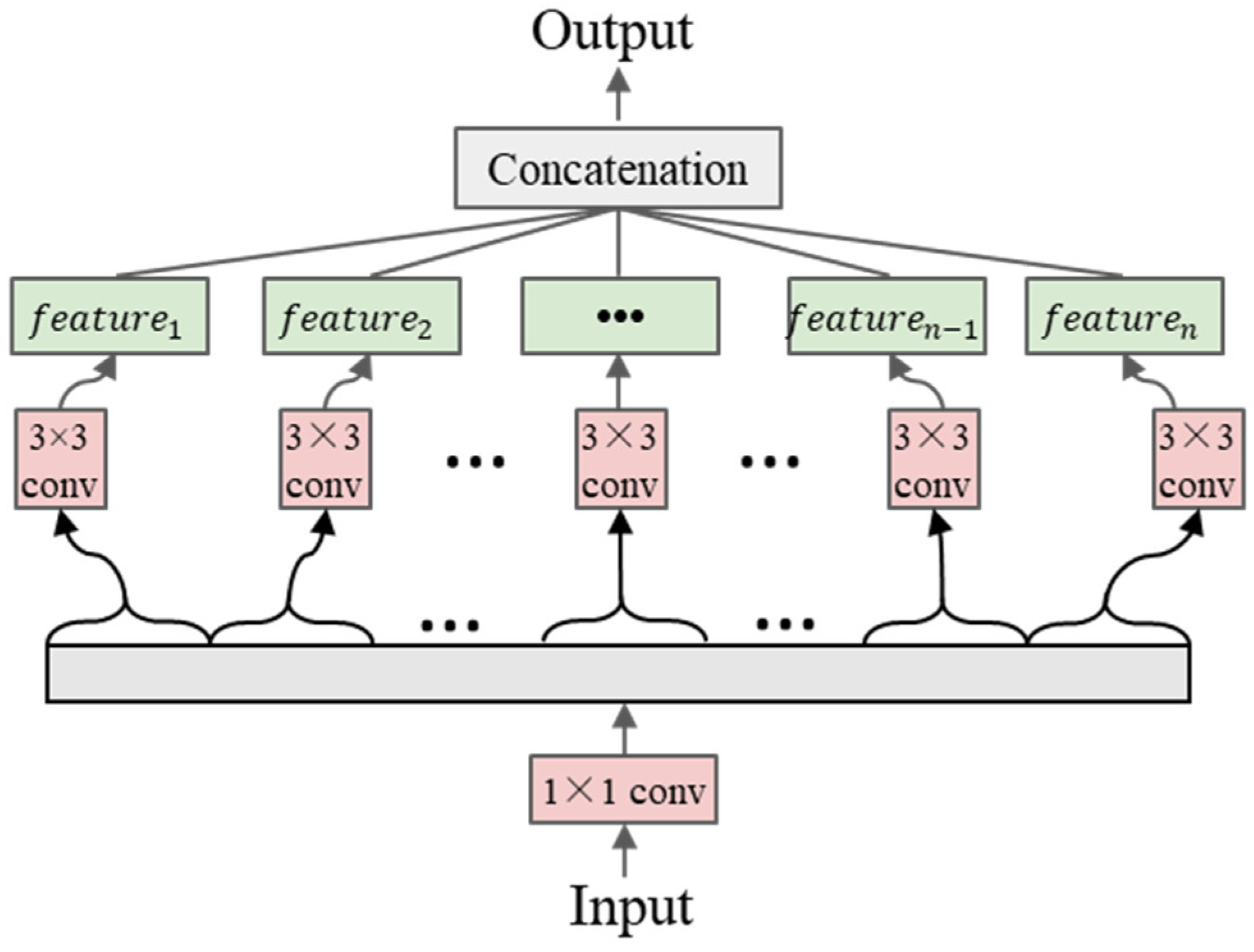
The deep semantic feature extraction module of the upper branch is based on CNN. To extract the rich semantic information of the LUSI data, a deep CNN, which is Xception [50], was used. As is known, CNN is used to extract semantic information by performing convolutional operations on the data obtained from the input layer. The traditional convolution is that the convolution kernel traverses the input data according to the step size, and each traversal multiplies the input value with the corresponding position of the convolution kernel and then adds the operation, and the feature matrix is obtained after traversal in turn. However, Xception is different. As shown in Figure 4, it designs the traditional convolution as a deeply separable convolution, i.e., point-by-point convolution and deep convolution. First, a convolution kernel of size 1 × 1 is used for point-by-point convolution to reduce the computational complexity; then, a 3 × 3 deep convolution is applied to disassemble and reorganize the feature map; simultaneously, ReLUs are not added to ensure that data are not corrupted. The whole network structure is stacked by multiple deep separable convolutions.

Compared to the traditional structure, Xception has four advantages: first, it uses cross-layer connections in the deep network to avoid the problem of degradation of the deep network, to make the network easier to train, and to improve the accuracy of the network; second, it uses the maximum pooling layer, which reduces the loss of information and improves the accuracy of the network; third, it uses the depth-separable convolutional layer, which reduces the number of parameters and improves the computational efficiency; and fourth, different sized images are used for training during the training process, which improves the robustness of the network.

Figure 5 shows a schematic of the flow of Xception to extract deep semantic features from the input data. The size of each DSFM is set to $h\times w\times d$, where $h$ denotes the height, $w$ donates the width of the DSFM, and $d$ denotes the channel dimension of the DSFM. Furthermore, we modified the last two layers of the Xception to use the new global average pooling (GAP) and fully connected layer (FCL).

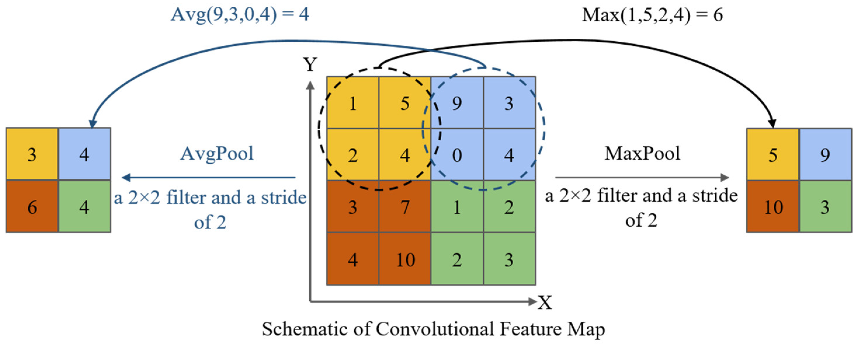
In the structure of Xception, the convolutional layer and the pooling layer generally appear at the same time. There are two main approaches to pooling: maximum pooling and average pooling. Maximum pooling retains the maximum value of each region as the result of the calculation, while average pooling is calculated by calculating the average value of each region as the result of the calculation. As shown in Figure 6, the 4 × 4 convolutional feature traversal is computed using the 2 × 2 filter according to the size of the step size of 2. Retaining the maximum value gives the maximum pooled feature map, and retaining the average value gives the average pooled feature map. Xception usually chooses a filter of size 3 × 3, traversed in 2 steps, to achieve maximum pooling.

The last DSFM processed by GAP is converted into an n-dimensional vector for easy classification by FCL. Its calculation is:

$$y_{out}(x_{in})=f(w^T{x}_{in}+b)$$

(2)

where $y_{out}$ is the output vector, $f$ is the activation function, $x_{in}$ is the input data with flattening the pooled DSFM to one-dimensional form, $w$ is the weight vector, and $b$ is the offset vector.

4.3. Spatial Structural Feature Map Extraction

As is known, CapsNet consists of an encoder and a decoder. The encoder consists of three layers, which serves to perform feature extraction on the input data; in addition, a routing process for computation between capsule layers and an activation function for capsule feature classification are included. The decoder is mainly composed of three FCLs and is used to ensure that the encoded information is reduced to the original input features. For the LUSC task, we mainly utilized the encoder part with adaptations.

For the rapid extraction of the rich structural information of the LUSI data while reducing the network parameters, inspired by the literature [27], the SSFM extraction module of the lower branch was built by using the graph routing-based CapsNet.

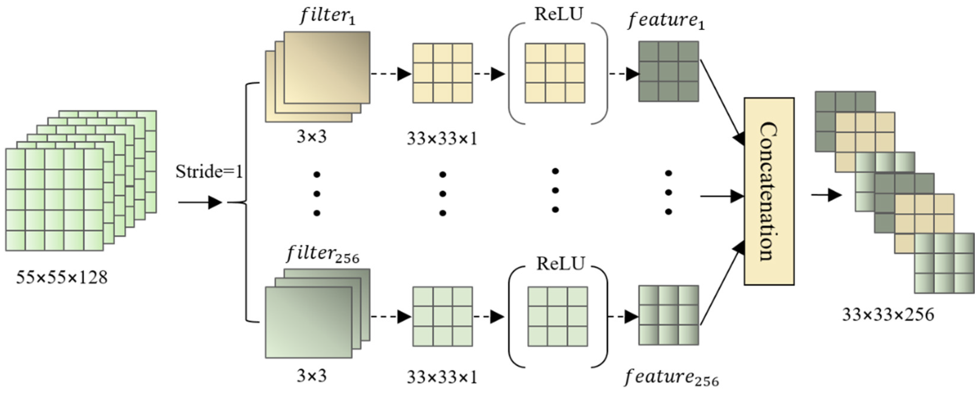
Specifically, it includes three important parts. The first part is to modify the original input layer to process the DSFMs of the upper branch. As shown in Figure 7, the shallow semantic feature map $F_{cnn}^{(i)}$ extracted by CNN are fine-tuned in size with convolutional operations to fit the input requirements of the CapsNet. The specific method is to use 256 convolution kernels of size 3 × 3 to perform convolution operations on the shallow semantic feature map in a traversal manner by step size 1. The ReLU function is also utilized to retain the values of the elements in the output features that are greater than 0, and the values of the other elements are set to 0. Finally, the 256 feature maps are stitched together by the cat function to form the input feature map $F_{cap}^{(i)}$ of the next layer.

The second part is to compute the primary capsule feature $F_{pcf}^{(i)}$ using the output feature map $F_{cap}^{(i)}$ of the previous layer. First, $N_{filter}$ convolution kernels of size 3 × 3 are utilized to carry out convolution operations in a traversal manner with a step size of 2 to obtain feature maps $F_{cap}^{(i_1)}$, where $N_{filter}=512/d_{incap}$; then, the output feature maps $F_{cap}^{(i_1)}$ are converted into a feature matrix $F_{cap}^{(i_2)}$ of the shape of $(b,p,d_{incap})$, where $d_{incap}$ denotes the number of primary capsules, the value of $p$ is the product of the square of the size of the feature after the convolution and the value of $N_{filter}$. Finally, the squash function is utilized to perform normalization on the new form of feature map $F_{cap}^{(i_2)}$ to obtain the main capsule feature map $F_{pcf}^{(i)}$, which is calculated as follows:

$$F_{pcf}^{(i)}=\frac{{‖F_{cap}^{(i_2)}‖}^2}{1+{‖F_{cap}^{(i_2)}‖}^2}\frac{F_{cap}^{(i_2)}}{‖F_{cap}^{(i_2)}‖}$$

(3)

When the modulus length of $F_{cap}^{(i_2)}$ tends to positive infinity, $F_{pcf}^{(i)}$ tends to 1; when the modulus length of $F_{cap}^{(i_2)}$ tends to 0, $F_{pcf}^{(i)}$ tends to 0. $F_{cap}^{(i_2)}/‖F_{cap}^{(i_2)}‖$ denotes the unit vector, which compresses the range of values of the modulus length of $F_{pcf}^{(i)}$ between [0, 1], keeping the feature direction unchanged, i.e., keeping the attributes of the image features represented by the feature unchanged.

The third part is the calculation of advanced capsule feature maps $F_{acf}^{(i)}$ using primary capsule feature maps $F_{pcf}^{(i)}$. After adding a dimension to the third dimension of feature map $F_{pcf}^{(i)}$, we obtain $F_{pcf}^{(i_1)}=(b,p,1,d_{incap})$, then we perform matrix multiplication operation with randomly initialized weight parameters $w_{pcf}^{(i_1)}=(b,p,d_{outcap})$ to get $F_{pcf}^{(i_2)}=(b,p,1,d_{outcap})$, where $d_{outcap}=2\times d_{incap}$, and then, we convert the feature map $F_{pcf}^{(i_2)}$ to $F_{pcf}^{(d_i)}=(b,p,d_{outcap})$, and finally input $F_{pcf}^{(d_i)}$ into the multiple graphs pooling module to obtain $F_{acf}^{(i)}$.

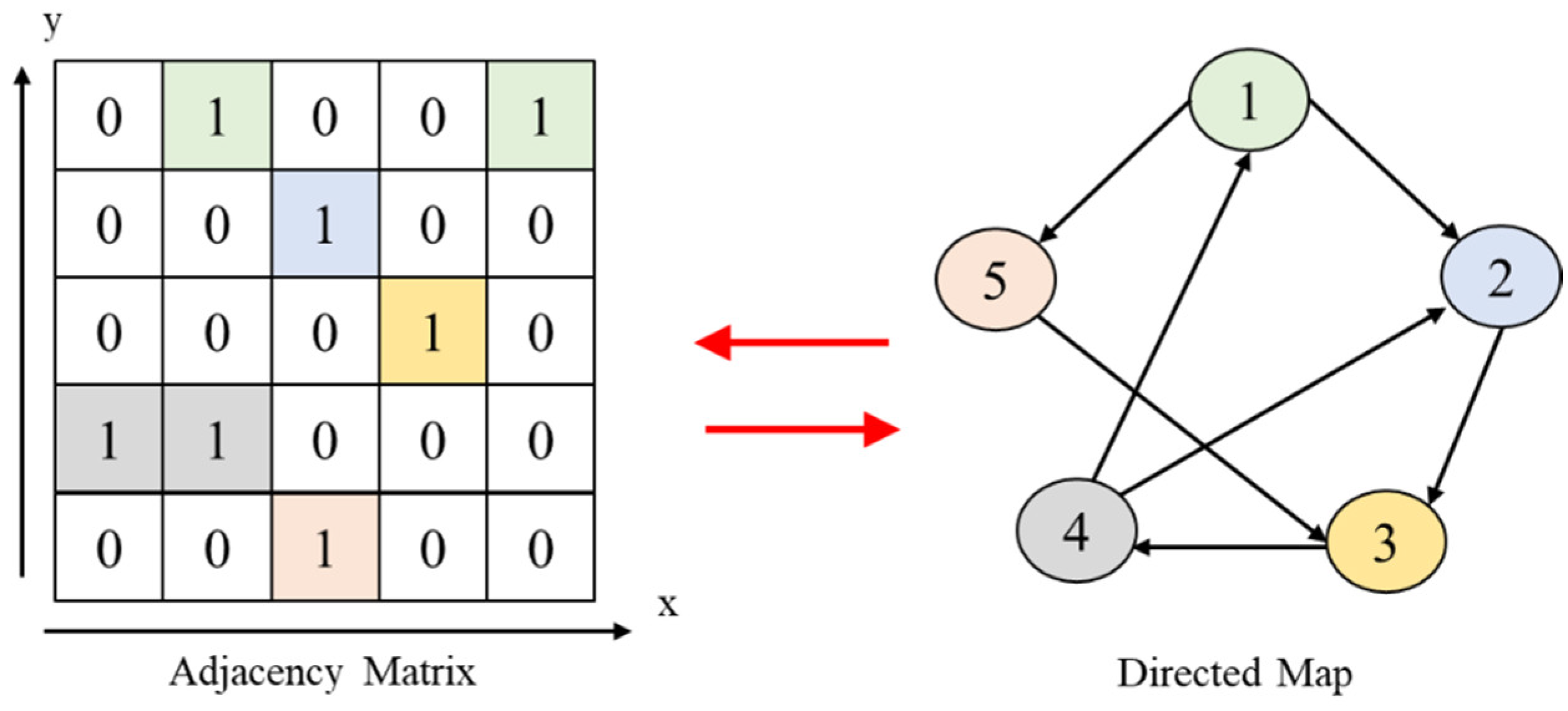
The multiple graphs pooling module serves to transform the primary capsule feature map $F_{pcf}^{(i)}$ into advanced capsule feature map $F_{acf}^{(i)}$, and the key technique is to calculate the weight coefficients $w_{acf}^{(i)}$ of each primary capsule feature map. Figure 8 shows a simple relationship between a two-dimensional array and an image.

The first step is to compute the nodes and edges of feature map $F_{pcf}^{(d_i)}$. Consider feature map $F_{pcf}^{(d_i)}=(b,p,d_{outcap})$ as $d_{outcap}$ graphs, where each single graph consists of $p$ nodes, and the vector $p$ can be seen as the feature map of the corresponding node.

The second step is to calculate the attention coefficients of the $d_{outcap}$ unigraph. Matrix multiplication of the adjacency matrix of the $d_{outcap}^{(i)}$ unigram is performed with the node features of the $d_{outcap}^{(i)}$ unigram, and then multiplied with the random initialization weight parameter $w$, and then the calculation result is inputted into the softmax function to obtain the attention coefficient $w_{acf}^{(d_i)}$ of the feature $F_{pcf}^{(d_i)}$.

$$w_{acf}^{(d_i)}=softmax(e^{-\frac{‖F_{pcf}^{(d_{ix})}‖-‖F_{pcf}^{(d_{iy})}‖}{2{\delta }^2}}\cdot F_{pcf}^{(d_i)}\cdot w)$$

(4)

where $F_{pcf}^{(d_i)}$ denotes the feature map of the $d_{outcap}^{(i)}$ dimension, and $d_{ix}$ and $d_{iy}$ denote the index of the feature map $F_{pcf}^{(d_i)}$ node, respectively.

The third step is to use multiply the attention coefficient with the node feature to obtain the attention feature, then the squash function is used to perform the normalization disposal to obtain the advanced capsule feature map $F_{acf}^{(i)}$.

$$F_{acf}^{(i)}=squash\left(\frac{1}{p}{\displaystyle \sum \left({(w_{acf}^{(d_i)})}^T\cdot F_{pcf}^{(d_i)}\right)}\right)$$

(5)

4.4. Feature Map Fusion and Scene Prediction

To obtain both DSFMs and SSFMs of the LUSIs, we designed a simple two-branch fusion module with different characteristics, where the feature maps extracted from the upper-branch CNN and the lower-branch CapsNet are integrated and inputted to the recognizer. The computational formulae used in this fusion module are as follows:

$$Z_j=f_w(F_{cnn}^{(1)})\oplus \left(\lambda \cdot \left({\displaystyle \sum _{i=1}^j{f}_{cap}(F_{cnn}^{(i)})}\right)\right)$$

(6)

where $Z_j$ denotes the fused feature, called DFM, $F_{cnn}^{(1)}$ denotes the last layer of semantic feature map extracted by the CNN, $f_w$ denotes the mean GAP and FCL, $\oplus$ denotes the use of summing according to the values of the corresponding elements one by one, $\lambda$ is the control coefficient, which denotes the key parameter controlling the deep fusion of the two-branch feature maps, and ${\displaystyle \sum _{i=1}^j{f}_{cap}(F_{cnn}^{(i)})}$ denotes the new spatial structure feature map formed by the CNN extracted feature maps input to the CapsNet after summing the corresponding elements.

After obtaining the DFM $Z_j$, it is first fed into the softmax function to calculate the probability of the image belonging to each class, and then the obtained probability values are used to calculate the predicted loss together with the probability values of the data labels after the image has been encoded by one-hot coding. While training the model using the HFCC-Net method, we used the cross-entropy loss function to obtain the minimum loss in both the training and validation datasets, achieving the task of optimizing the weight parameters of the model. Equation (7) lists the loss values obtained for a batch size of land-use data after softmax function and cross-entropy loss calculation.

$$loss(b,c)=-\frac{1}{b}{\displaystyle \sum _{i=1}^b{\displaystyle \sum _{j=1}^c{y}_{ij}\log \left(e^{z_i}/{\displaystyle \sum _{j=1}^c{e}^{z_{ij}}}\right)}}$$

(7)

where $b$ denotes the number of the LUSI, $c$ denotes the number of categories of land-use scenes, $j$ denotes the true probability value of the $i$-th scene data label (if the true category of the $i$-th scene data label is equal to $j$ then, $y_{ij}$ is equal to 1, otherwise 0), and $y_{ij}$ denotes the predicted probability that the $i$-th scene image data belongs to category $j$-th.

5. Results

5.1. Experimental Conditions

5.1.1. Platform Settings

To verify the outstanding performance of our proposed method in the LUSC task, we used Python3.7 language to build the HFCC-Net network framework under Pytorch framework, and fully trained on a Windows 10 operating system using each of the four classification datasets talked about in Section 3 to verify the advancement of HFCC-Net. Specifically, we use NVIDIA GPU acceleration during the training process to increase the speed of model training and inference. The specific environment configuration is shown in

Table 3. Parameters for the platforms.

Platforms		Parameters
Hardware	Processor	Intel(R) Xeon(R) W-2245 CPU
	RAM	128 GB
	Graphics card	NVIDIA RTX A6000
	Memory	48 GB
Software	Operating system	Windows 10
	Operational environment	Python 3.7
	Deep learning framework	Pytorch

below:

5.1.2. Training Details

To facilitate the comparison and analysis of the classification performance of HFCC-Net, we randomly selected 20%, 50%, and 80% of the four datasets as the training data, and the corresponding 80%, 50%, and 20% of the data as the test data, respectively. When inputting the data into the HFCC-Net model, we set the size of the images to 224 × 224, and the number of images inputted in each batch was set to 64, and each dataset was trained five times, with 200 rounds each time, and the mean and standard deviation of SCA were counted.

In the training process, we choose the cross-entropy loss function to describe the difference between the image category results predicted by HFCC-Net and the real image categories; in order to effectively deal with the gradient noise and non-smoothness in the learning process, we used Adam’s algorithm to update the parameters of the HFCC-Net network. In addition, for speeding up the convergence speed while avoiding overfitting, the learning rate takes the value of 0.0001 and the weight decay coefficient takes the value of 0.0005.

5.2. Experimental Results

5.2.1. Results on the RSSCN

Table 4. SCA on the RSSCN.

Practical Method	Classification Results (SCA, %)
	50% for Training	20% for Training
GoogleNet [29]	85.84 ± 0.92	82.55 ± 1.11
Two-stage fusion [36]	92.37 ± 0.72	-
VGG-VD-16 [29]	87.18 ± 0.94	83.98 ± 0.87
TEX-Net-LF [34]	94.00 ± 0.55	92.45 ± 0.45
Dual-attention [35]	93.25 ± 0.28	91.07 ± 0.65
CaffeNet [29]	88.25 ± 0.62	85.57 ± 0.95
Deep filter banks [37]	90.40 ± 0.60	-
LCNN-BFF [51]	94.64 ± 0.21	-
EfficientNetB3-Attn-2 [52]	96.17 ± 0.23	93.30 ± 0.19
EfficientNetB3-Basic [52]	94.39 ± 0.10	92.06 ± 0.39
HFCC-Net	95.30 ± 0.24	93.61 ± 0.47

shows the SCA obtained by 10 different algorithms trained on the RSSCN dataset. In order to achieve the best classification results, we set the structural parameters of HFCC-Net, i.e., $j$ takes the value of 2, $\lambda$ takes the value of 1, $d_{incaps}$ takes the value of 32, and $d_{outcaps}$ takes the value of 64. The experimental data obtained show that when 50% of the training data are used for learning, HFCC-Net can achieve 95.30% of the average accuracy for 50% of the test data; when 20% of the training data are used for learning, HFCC-Net can achieve 93.61% of the average accuracy for 80% of the test data. Comparing the SCA values under similar experimental conditions, it can be seen that the SCAs obtained by HFCC-Net with different training data are all significantly competitive. Specifically, the average accuracy using HFCC-Net is improved by 0.66 compared with the method [51] that only fuses different DSFMs, and the SCA of HFCC-Net is relatively high when LUSI is used for training with relatively less data compared to the method that enhances DSFMs with attentional mechanisms [52].

To further analyze the ability of HFCC-Net to classify images of each category, we utilize the best model obtained from training data of the RSSCN to classify the test data and view the misclassification between images of each category.

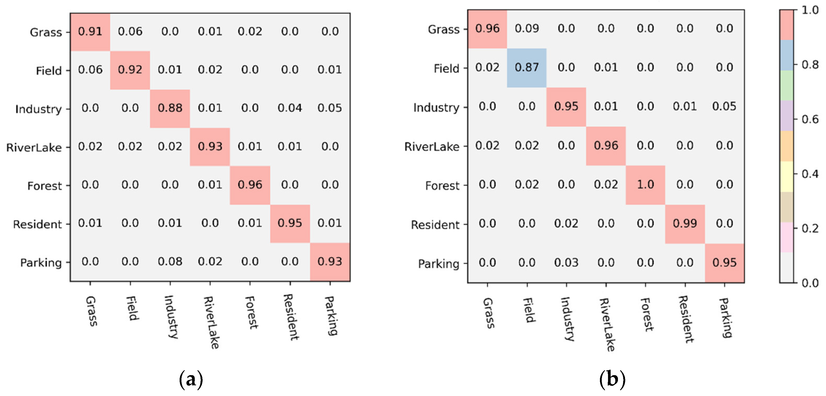
Figure 9a shows the image category misclassification obtained by classifying the test data with a 50% share of the data using the best model obtained after training in the data with a 50% share of the data. Among the seven image categories of the RSSCN, the most accurately classified category is ‘Forest’, which has a classification probability of 0.96; ‘Industry’ and ‘parking’ because of their similar structure. ‘Industry’ is classified with a probability of 0.88 because of its similar structure; however, the average probability of the overall classification accuracy of the images in the other categories is greater than 0.90; Figure 9b illustrates the best model obtained by using the model trained on 20% of the test data, and the best model obtained by using the model trained on 80% of the test data. The most accurately classified category is ‘Forest’, with a probability of accuracy of 1. ‘Grass’ and ‘Field’ have similar structure, which causes the model to classify ‘Grass’ as grass, however, the average probability of other categories of images being classified accurately is greater than 0.95, which also proves the sophistication of our method.

5.2.2. Results on the SIRI

Table 5. SCA on the SIRI.

Practical Method	Classification Results (SCA, %)
	50% for Training	80% for Training
ResNet-50 [25]	94.67	95.63
AlexNet [25]	82.50	88.33
VGG-16 [25]	94.42	96.25
Fine-tuning MobileNetV2 [32]	95.77 ± 0.16	96.21 ± 0.31
Siamese ResNet-50 [33]	95.75	97.50
Siamese AlexNet [33]	83.25	88.96
Siamese VGG-16 [33]	94.50	97.30
Siamese CapsNet [25]	94.37	96.99
DenseNet + DenseNet [54]	-	96.37
DenseNet + VGG-16 [54]	-	94.16
MSAA-Net [53]	-	95.21 ± 0.65
HFCC-Net	96.72 ± 0.43	97.78 ± 0.41

shows the SCA obtained by 11 different algorithms trained on the SIRI dataset. In order to achieve the best classification results, we set the structural parameters of HFCC-Net, i.e., $j$ takes the value of 2, $\lambda$ takes the value of 1, $d_{incaps}$ takes the value of 32, and $d_{outcaps}$ takes the value of 64. While using 50% of the training data for learning, HFCC-Net can achieve an average accuracy of 96.72% with 50% of the testing data; comparing the values of SCA, it can be seen that our method has higher accuracy under similar experimental conditions. e.g., 0.97 improvement over the average accuracy obtained by using the Siamese ResNet-50 [33], 2.35 improvement over the average accuracy obtained with the Siamese CapsNet [25], etc. When learning with 80% of the training data, HFCC-Net can achieve an average accuracy of 97.78% with 20% of the test data. Similarly, our method achieves better classification results, e.g., 0.28 improvement in average accuracy over the Siamese ResNet-50 [33], 0.79 improvement in average accuracy over the Siamese CapsNet [25], and better SCA for HFCC-Net compared to the state-of-the-art methods [53,54].

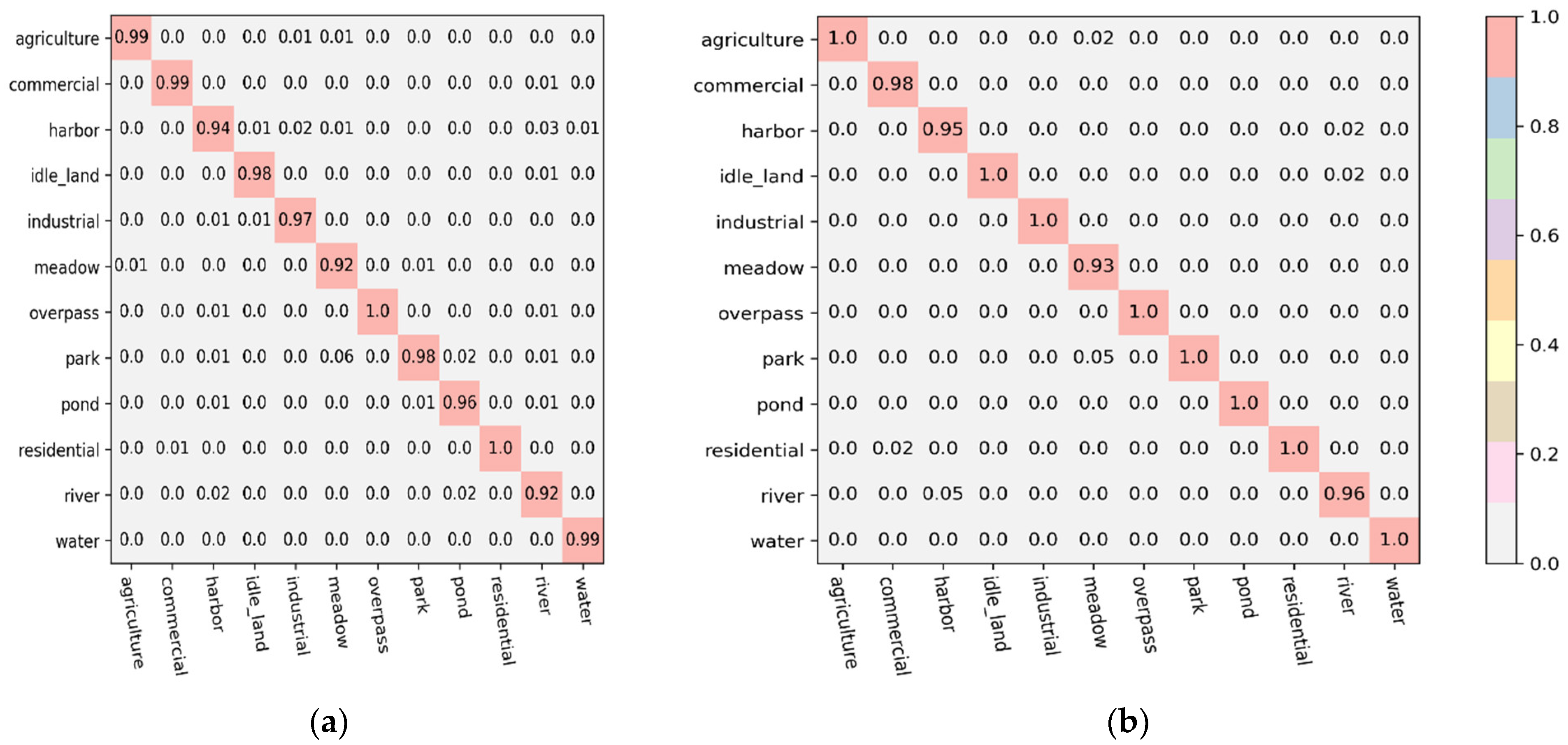
Figure 10a shows the misclassification of image categories obtained by classifying the test data with a 50% share of the data using the best model obtained after training in the data with a 50% share of the data. Among the 12 image categories of the SIRI, the most accurately classified are “Overpass” and “residential”, whose classification probability is 1; the average probability of overall classification accuracy for all categories of images is not less than 0.92; Figure 9b shows the average probability of overall classification accuracy for all categories, 0.92; Figure 10b shows the image category misclassification obtained by classifying 20% of the test data using the best model obtained after training on 80% of the data. The most accurately classified categories are “idle_land”, “industrial”, “overpass”, “park”, “pond”, “residential” and “water”, the probability of accuracy is 1; the average probability of an image being accurately classified for all categories is not less than 0.93.

5.2.3. Results on the UCM

Table 6. SCA on the UCM.

Practical Method	Classification Results (SCA, %)
	50% for Training	80% for Training
VGG-VD-16 [29]	94.14 ± 0.69	95.21 ± 1.20
GoogLeNet [29]	92.70 ± 0.60	94.31 ± 0.89
GBNET [30]	95.71 ± 0.19	96.90 ± 0.23
GBNET+Global feature [30]	97.05 ± 0.19	98.57 ± 0.48
CaffeNet [29]	93.98 ± 0.67	95.02 ± 0.81
Two-stream fusion [31]	96.97 ± 0.75	98.02 ± 1.03
ARCNET-VGG16 [38]	96.81 ± 0.14	99.12 ± 0.40
Inception-v3-CapsNet [16]	97.59 ± 0.16	99.05 ± 0.24
LCNN-BFF [51]	-	99.29 ± 0.24
EfficientNetB3-Attn-2 [52]	97.90 ± 0.36	99.21 ± 0.22
EfficientNetB3-Basic [52]	97.63 ± 0.06	98.73 ± 0.20
VGG-16-CapsNet [16]	95.33 ± 0.18	98.81 ± 0.22
HFCC-Net	98.38 ± 0.18	99.20 ± 0.46

shows the SCA obtained by 12 different algorithms trained on the UCM dataset. To achieve the best classification results, we set the structural parameters of HFCC-Net, i.e., $j$ takes the value of 2, $\lambda$ takes the value of 1, $d_{incaps}$ takes the value of 32, and $d_{outcaps}$ takes the value of 64. The experimental data obtained show that when using 50% of the training data for learning, HFCC-Net in 50% of the test data can achieve an average accuracy of 98.38%; a comparison of the values of SCA shows that under similar experimental conditions, our method has a higher SCA, e.g., an increase of 0.79 over the average accuracy obtained using Inception-v3-CapsNet [16] and the average accuracy improvement over the average accuracy obtained using VGG-16-CapsNet [16] is 3.05. When learning with 80% of the training data, HFCC-Net achieves 99.20% with 20% of the test data; similarly, our method improves the average accuracy over Inception-v3-CapsNet [16] by 0.15, and over VGG-16-CapsNet [16] by average accuracy by 0.39. In addition, HFCC-Net is more competitive compared to state-of-the-art methods [51,52] in classification.

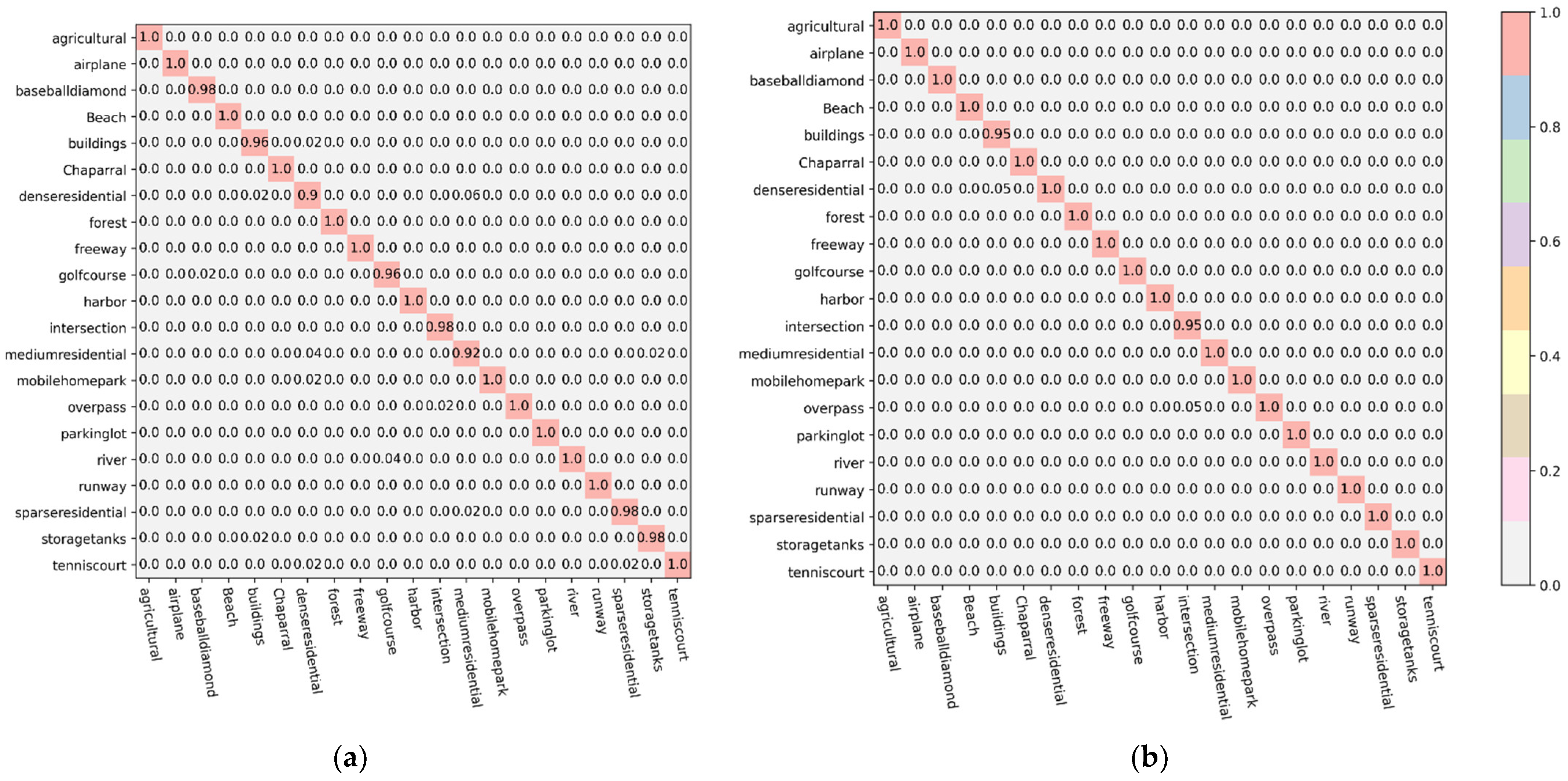
The best model obtained using the training data of the UCM was utilized to classify the test data and to see the misclassification between each category of images. Figure 11a shows the misclassification of image categories obtained by classifying the test data with a 50% share of the data using the best model obtained after training in the data with a 50% share of the data. Among the 21 image categories of the UCM, “baseball diamond”, “buildings”, “dense residential”, “golf course”, “intersection”, “medium residential”, “sparse residential”, and “storage tanks” are accurately classified with a probability close to 1, while the other categories are classified with a probability of 1. Figure 11b shows the best model obtained using the data trained on 80% of the data. Figure 11b shows the image category misclassification obtained by classifying the test data with 20% of the data using the best model obtained after training on 80% of the data. The probability of accurately classifying “buildings” and “intersection” is close to 1, while the probability of classifying the other categories is 1.

5.2.4. Results on the OPTIMAL

Table 7. SCA on the OPTIMAL.

Practical Method	Classification Results (SCA, %)
	80% for Training
Fine-tuning VGGNet16 [29]	87.45 ± 0.45
Fine-tuning GoogLeNet [29]	82.57 ± 0.12
GBNET [30]	91.40 ± 0.27
GBNET+Global feature [30]	93.28 ± 0.27
Fine-tuning AlexNet [38]	81.22 ± 0.19
VGG-VD-16 [29]	87.45 ± 0.45
ARCNET-ResNet34 [38]	91.28 ± 0.45
ARCNET-VGGNet16 [38]	92.70 ± 0.35
ARCNET-AlEXNET [38]	85.75 ± 0.35
SopNet-GCN-ResNet50 [39]	93.37 ± 0.68
SopNet-GAT-ResNet50 [39]	93.55 ± 0.74
EfficientNetB3-Attn-2 [52]	95.86 ± 0.22
EfficientNetB3-Basic [52]	94.76 ± 0.26
HFCC-Net	94.80 ± 0.89

shows the SCA obtained by 13 different algorithms trained on the OPTIMAL dataset. To achieve the best classification results, we set the structural parameters of HFCC-Net, i.e., $j$ takes the value of 2, $\lambda$ takes the value of 0.2, $d_{incaps}$ takes the value of 32, and $d_{outcaps}$ takes the value of 64. The obtained experimental data show that HFCC-Net can achieve an average accuracy of 94.80% with 20% of the test data when learning with 80% of the training data. Comparing the values of SCA, it can be seen that under similar experimental conditions, our method has a higher SCA, e.g., HFCC-Net improves the average accuracy by 1.43 over the average accuracy obtained by SopNet-GCN-ResNet50 [39], and 1.25 over the average accuracy obtained by using SopNet-GCN-ResNet50 [39], and even reaches the level of a CNN-based state-of-the-art method [52].

Using the best model obtained from the training data of the OPTIMAL, we classify the test data and see the misclassification between each category of images. Figure 12 shows the misclassification of image categories obtained by using the best model obtained after training in the data with a share of 80% to classify the test data with a share of 20%. Among the 31 image categories of the OPTIMAL, “intersection” and “commercial area” have a similar structure, resulting in some “intersection” being classified as “commercial area”; “mountain” and “desert” have similar structures, resulting in some “mountain” being classified as “desert”; “railway” and “runway” have similar structures, resulting in some “railway” being classified as “runway”. Surprisingly enough, the probability of classification for the other 28 categories is close to 1.

5.3. Discussion

5.3.1. Combinatorial Patterns of DSFMs

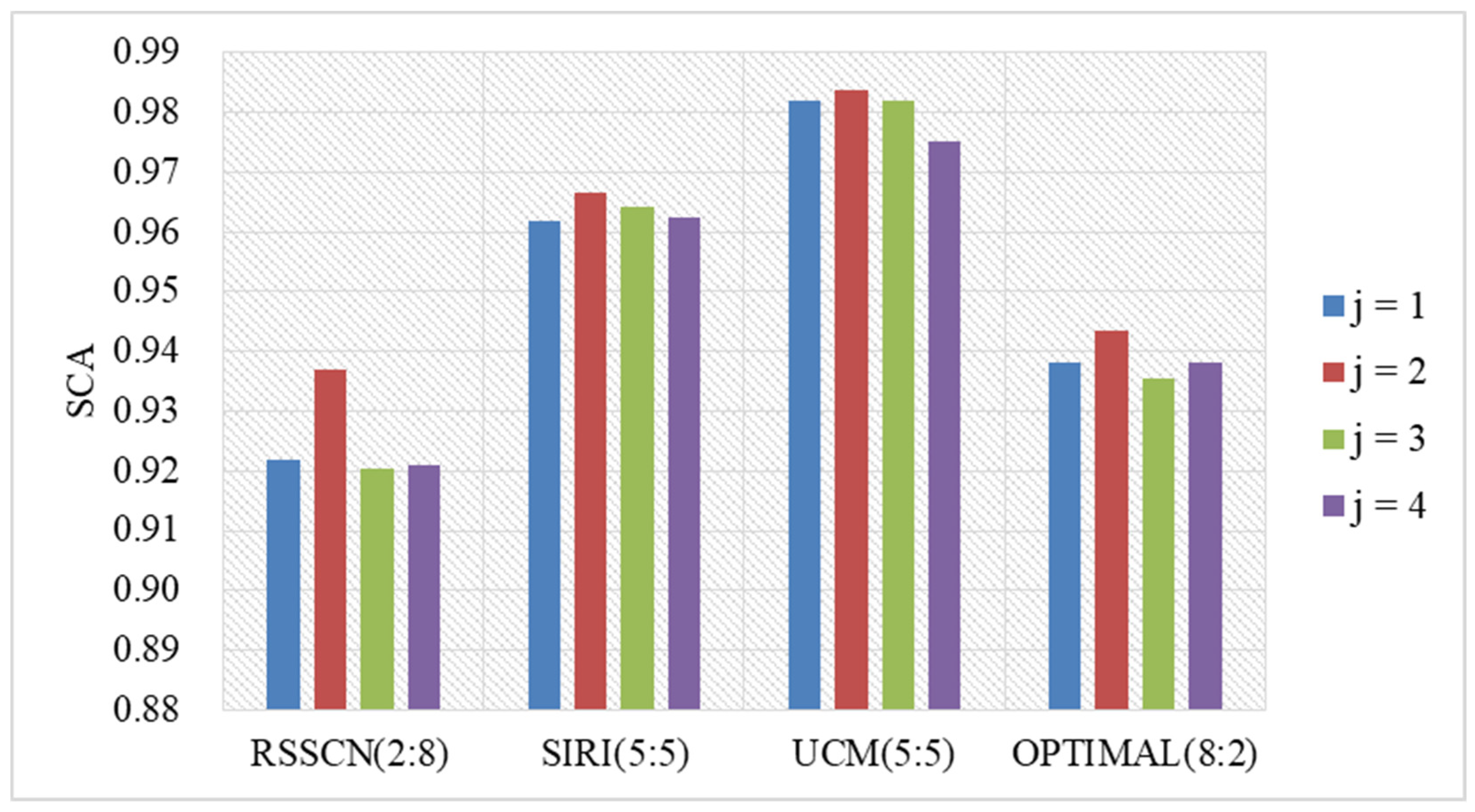
As can be seen from Figure 2, the SSFMs of the lower branch of HFCC-Net are obtained by inputting the deep semantic features of the upper branch into the graph routing-based CapsNet. In order to further verify the outstanding contribution of our selected DSFMs to the classification performance of HFCC-Net, we conducted an ablation study on the inputs of the lower-branch CapsNet. The specific idea is to select one, two, three, and four feature maps as the input feature maps of the lower branch. Considering that the increasing number of convolutional layers tends to cause layer-by-layer loss of image information and that the current CapsNet is more suitable for small-size image features, we focus on the middle- and high-level features of the upper branch when selecting semantic feature maps. The specific input feature maps are shown in

Table 8. Input feature maps for the lower branch.

Total	DSFMs	Discriminative Feature Maps
1	$F_{cnn}^{(4)}$	$Z_1=f_w(F_{cnn}^{(1)})\oplus (\lambda \cdot f_{cap}(F_{cnn}^{(4)}))$
2	$F_{cnn}^{(4)}$,$F_{cnn}^{(3)}$	$Z_2=f_w(F_{cnn}^{(1)})\oplus (\lambda \cdot f_{cap}(F_{cnn}^{(4)},F_{cnn}^{(3)}))$
3	$F_{cnn}^{(4)}$, $F_{cnn}^{(3)}$, $F_{cnn}^{(2)}$	$Z_3=f_w(F_{cnn}^{(1)})\oplus (\lambda \cdot f_{cap}(F_{cnn}^{(4)},F_{cnn}^{(3)},F_{cnn}^{(2)}))$
4	$F_{cnn}^{(4)}$, $F_{cnn}^{(3)}$, $F_{cnn}^{(2)}$, $F_{cnn}^{(1)}$	$Z_4=f_w(F_{cnn}^{(1)})\oplus (\lambda \cdot f_{cap}(F_{cnn}^{(4)},F_{cnn}^{(3)},F_{cnn}^{(2)},F_{cnn}^{(1)}))$

.

Under the premise that other experimental conditions remain unchanged, we utilized four kinds of the LUSI to start training separately. Based on the experience, the value of $\lambda$ is tentatively set to 1. By selecting the best training model under the four inputs, we performed classification prediction on the test data, and obtained the accuracy of HFCC-Net for the four datasets under four different inputs of DSFMs. As shown in Figure 13, when the input method of $j=2$, better classification results can be obtained.

5.3.2. Control Coefficient for Dual-Branch Feature Fusion

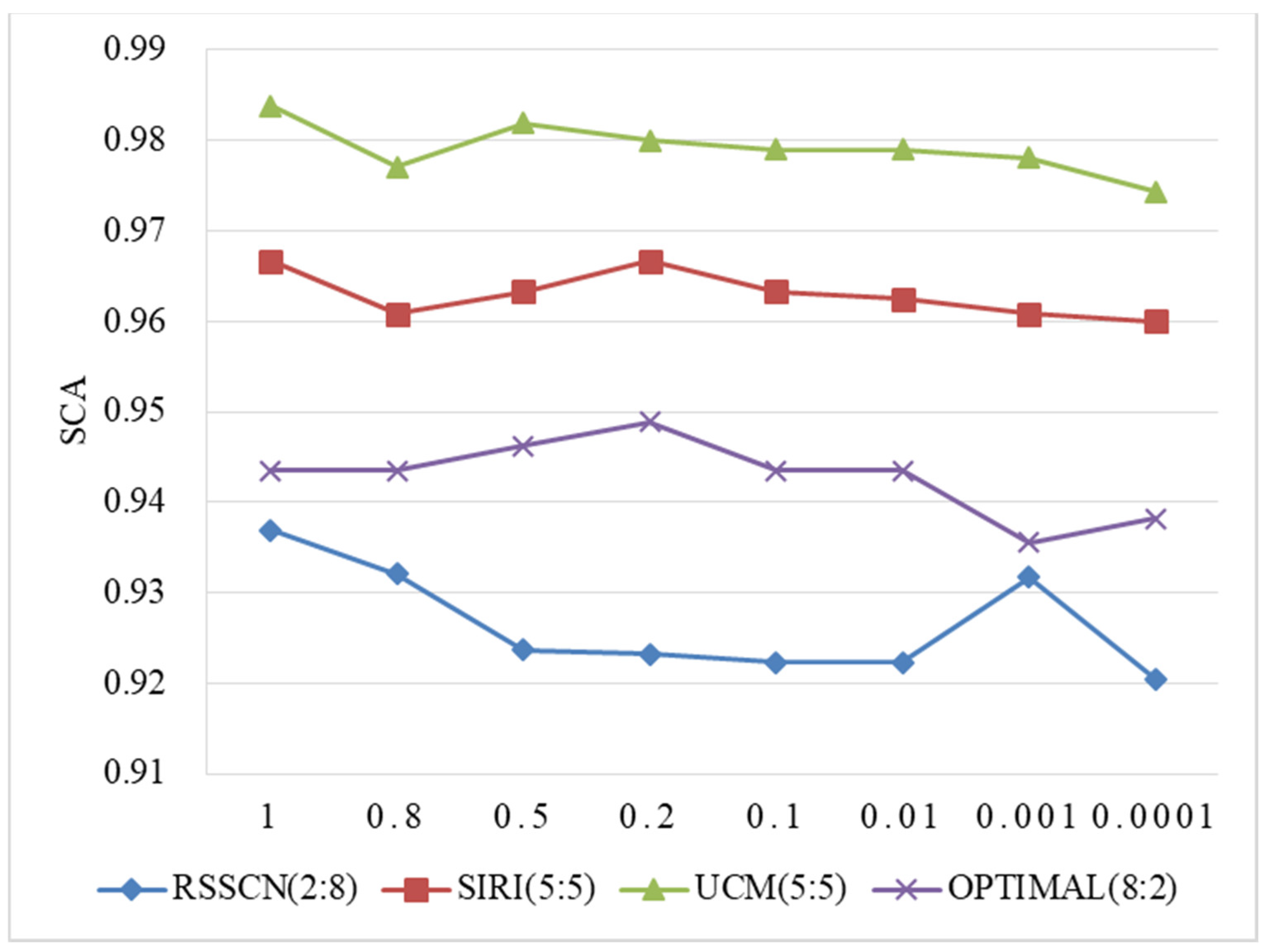
There are three main fusion methods for DSFMs: one is to splice different convolutional feature maps in channel dimension; one is to add different convolutional feature maps element-by-element; and one is to multiply two convolutional feature maps element-by-element. After extensive experiments using HFCC-Net in different fusion ways, we find that the element-by-element summation has an important contribution to the classification of the model. In addition, in order to speed up the network convergence and maximize the advantages of the DSFM and SSFM, we discuss the performance of the HFCC-Net model with different fusion control coefficients.

When performing the fusion of the corresponding elements of discriminative feature maps, considering that the SSFMs are special and the values of the elements are large relative to the DSFMs, we discuss how the different control coefficients $\lambda$ of all the elements of the SSFMs affect the fusion effect. Specifically, the discussion process is divided into two steps: first the order of magnitude of $\lambda$ is determined, in accordance with the multiples of 10 to deflate, and we found that when the control coefficient takes 1, a higher classification accuracy can be obtained; and then we determined more specific control coefficients, and following with the law of the equivariant series, we chose to carry out experiments on the three special values of 0.8, 0.5, and 0.2.

The optimal fusion control coefficients for HFCC-Net differ across the four datasets because of the variability in the image content of the land-use scenes and because of the differences in the amount of data in the categories of the scene images. Under the premise that other experimental conditions remain unchanged, the SCA we obtained on the predicted datasets of the four datasets are shown in Figure 14, which shows that when $\lambda$ takes the value of 1, the effect of feature map fusion can promote HFCC-Net to achieve the better classification performance on the RSSCN, SIRI, and UCM datasets; when the value is taken as 0.2, the effect of feature map fusion is more suitable for the OPTIMAL dataset.

5.3.3. Input and Output Dimensions of Capsules

A capsule is the basic unit of CapsNet, similar to a neuron, which is able to extract richer feature representation. Specifically, each capsule represents a feature map, and increasing the number of capsules increases the expressive power of the network, allowing it to capture more details and complex feature maps. However, the increase also increases the computational and storage overhead of the network. Too many capsules may cause the network to overfit the training data, reducing its ability to generalize to new data. In addition, if the number of capsules is not set properly, it may lead to training difficulties such as gradient vanishing or gradient explosion.

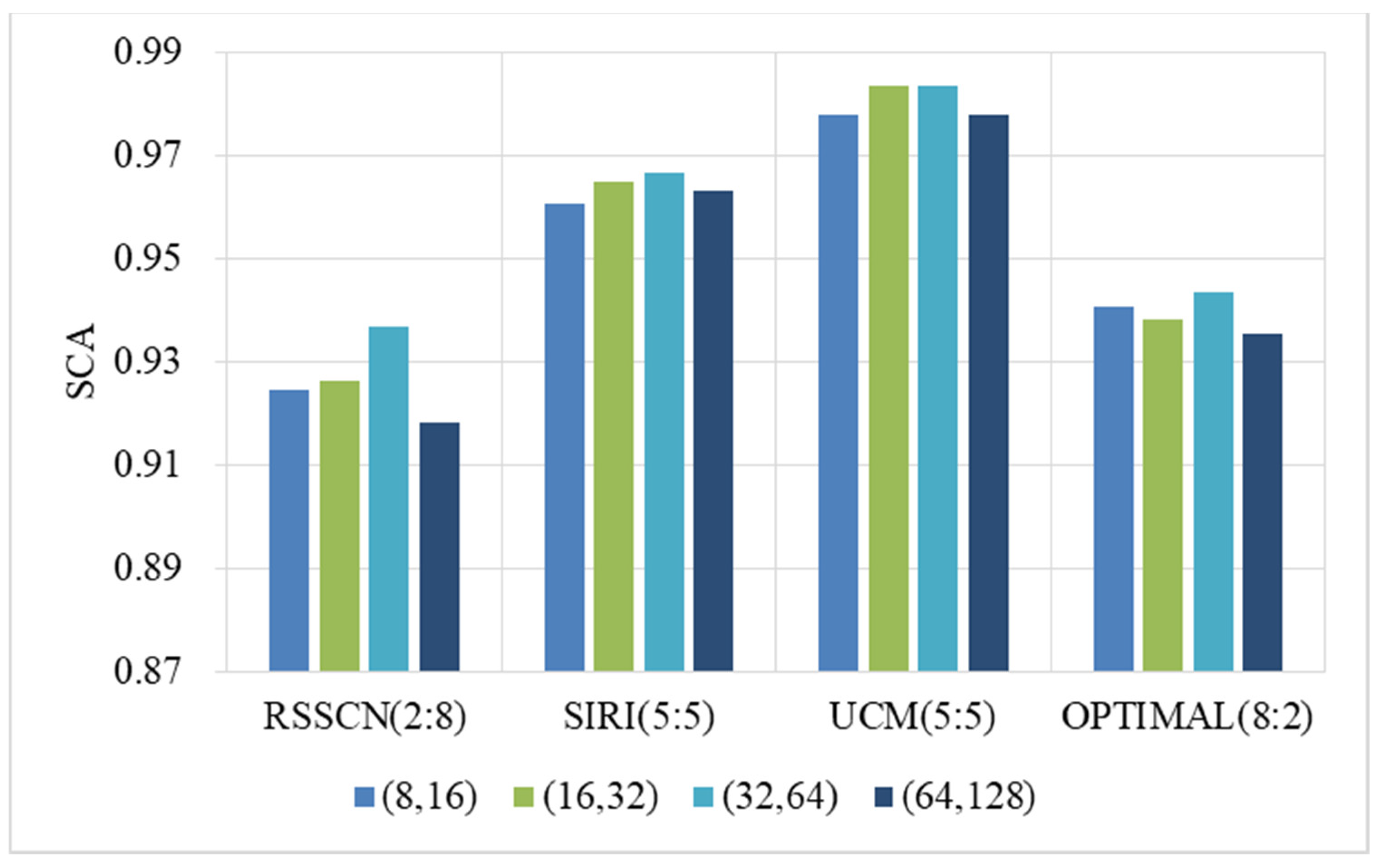
We have designed four different combinations of capsule sizes in HFCC-Net based on the characteristics of the down-branch network and the input data. Specifically, the dimensions of the input capsules $d_{incaps}$ are sequentially designed as 8, 16, 32, and 64, and the dimensions of the output capsules $d_{outcaps}$ are correspondingly designed as 16, 32, 64, and 128. Other conditions are kept unchanged, and the SCA of the HFCC-Net model is obtained after training on four LUSI datasets as shown in Figure 15. It can be seen that HFCC-Net can achieve a better classification performance when the dimension of the input capsules $d_{incaps}$ is set to 32 and the dimension of the output capsules $d_{outcaps}$ is set to 64.

5.3.4. Different Backbone Network Architecture

The backbone network can capture local information such as spatial structure, texture, and edges of the input data, as well as higher-level semantic and contextual information, and the goodness of the backbone network is directly related to the performance and performance of the whole deep learning system.

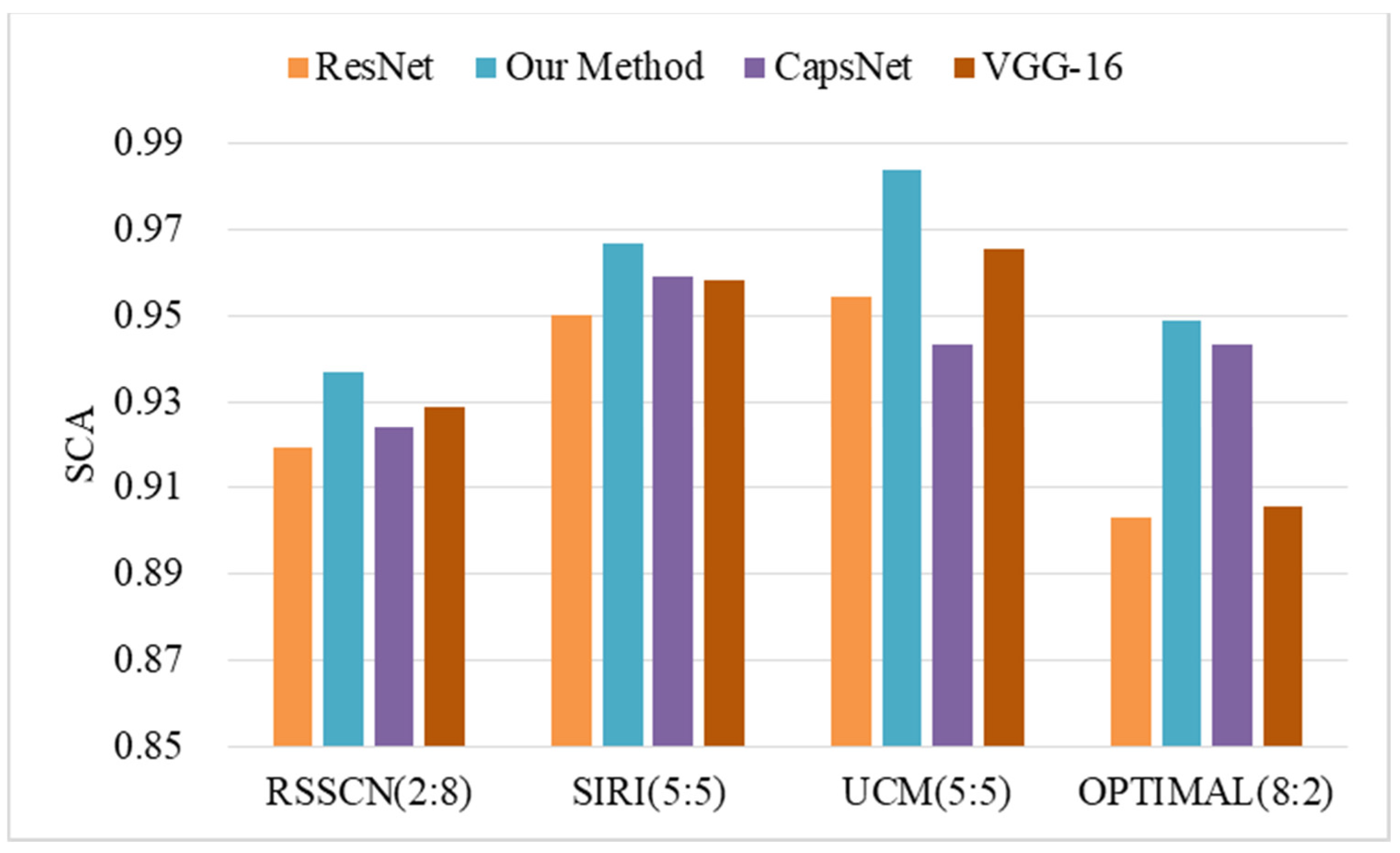
To analyze the goodness of the HFCC-Net backbone network, we conducted a comparative experiment. Specifically, we first selected two powerful feature extraction CNNs as the upper-branch backbone networks. The first time, we extracted the semantic features of the conv2_x and conv3_x layers using ResNet-50 [55], and used the two features as the input information of the HFCC-Net under-branch network; the second time, we extracted the semantic features of the conv3_256 and conv4_512 layers using VGG-16 [56], and used them as the HFCC-Net under-branch network’s inputs; other experimental conditions are kept constant, and our obtained SCAs on the four datasets are shown in Figure 16. It can be seen that compared with the two typical backbones, the upper branching network of HFCC-Net has a more obvious promotion effect on SCA. Similarly, we selected the most popular CapsNet as the lower-branch backbone network to compare and verify the feature extraction ability of the lower branch of HFCC-Net. Different from the method adopted by HFCC-Net, CapsNet [12] uses a dynamic routing mechanism as the information transfer method. We take $F_{cnn}^{(3)}$ and $F_{cnn}^4$ of the Xception network as the input of CapsNet, and obtain the spatial structure features of the image through the dynamic routing mechanism. After the experiments, it can be seen that compared with CapsNet, the lower branch network of HFCC-Net promotes SCA more obviously in the LUSI datasets.

6. Conclusions

CNN-based techniques for the LUSC are techniques that have emerged in recent years, which could autonomously learn information-rich features from the original pixels of RSI, and automatically complete the classification with high accuracy. However, the pooling layer of CNN leads to more data loss the more convolutional layers it has. Moreover, CNN does not utilize the spatial structure features between individual objects in the image content. Therefore, it is extremely challenging to improve the classification accuracy of CNN for complex LUSI. CapsNet is a novel neural network that better captures the structural relationships between the contents in an image through capsule units. To improve the SCA of the LUSC and make up for the shortcomings of CNN methods, we propose a dual-branch hybrid framework, HFCC-Net, which makes more complete use of the LUSI’s global semantic and local structural information. DSFM of RSI is extracted by using the transfer learning technique, SSFM is obtained by using the shallow DSFM as the input of CapsNet, and the DFMs of the two branches are fused in turn by using the newly designed fusion function and finally the DFMs are input into the classifier to obtain the predictive probability of the LUSI. The experimental results on four public datasets prove the effectiveness of HFCC-Net, and in future work, we plan to improve the CNN, such as adding the attention mechanism, to further improve the classification accuracy of the model.

References

1. Dutta, S.; Das, M. Remote sensing scene classification under scarcity of labelled samples—A survey of the state-of-the-arts. Comput. Geosci. 2023, 171, 105295. [Google Scholar] [CrossRef]
2. Cheng, G.; Xie, X.; Han, J.; Guo, L.; Xia, G.-S. Remote sensing image scene classification meets deep learning: Challenges, methods, benchmarks, and opportunities. IEEE J. Sel. Top. Appl. Earth Obs. Remote Sens. 2020, 13, 3735–3756. [Google Scholar] [CrossRef]
3. Wang, J.; Li, W.; Zhang, M.; Tao, R.; Chanussot, J. Remote Sensing Scene Classification via Multi-Stage Self-Guided Separation Network. IEEE Trans. Geosci. Remote Sens. 2023, 61, 5615312. [Google Scholar]
4. Huang, X.; Liu, F.; Cui, Y.; Chen, P.; Li, L.; Li, P. Faster and Better: A Lightweight Transformer Network for Remote Sensing Scene Classification. Remote Sens. 2023, 15, 3645. [Google Scholar] [CrossRef]
5. Zhang, J.; Zhao, H.; Li, J. TRS: Transformers for remote sensing scene classification. Remote Sens. 2021, 13, 4143. [Google Scholar] [CrossRef]
6. Thapa, A.; Horanont, T.; Neupane, B.; Aryal, J. Deep Learning for Remote Sensing Image Scene Classification: A Review and Meta-Analysis. Remote Sens. 2023, 15, 4804. [Google Scholar] [CrossRef]
7. Khatami, R.; Mountrakis, G.; Stehman, S.V. A meta-analysis of remote sensing research on supervised pixel-based land-cover image classification processes: General guidelines for practitioners and future research. Remote Sens. Environ. 2016, 177, 89–100. [Google Scholar] [CrossRef]
8. Kavzoglu, T.; Tonbul, H. An experimental comparison of multi-resolution segmentation, SLIC and K-means clustering for object-based classification of VHR imagery. Int. J. Remote Sens. 2018, 39, 6020–6036. [Google Scholar] [CrossRef]
9. Maurya, K.; Mahajan, S.; Chaube, N. Remote sensing techniques: Mapping and monitoring of mangrove ecosystem—A review. Complex Intell. Syst. 2021, 7, 2797–2818. [Google Scholar] [CrossRef]
10. Ma, L.; Liu, Y.; Zhang, X.; Ye, Y.; Yin, G.; Johnson, B.A. Deep learning in remote sensing applications: A meta-analysis and review. ISPRS J. Photogramm. Remote Sens. 2019, 152, 166–177. [Google Scholar] [CrossRef]
11. Song, J.; Gao, S.; Zhu, Y.; Ma, C. A survey of remote sensing image classification based on CNNs. Big Earth Data 2019, 3, 232–254. [Google Scholar] [CrossRef]
12. Sabour, S.; Frosst, N.; Hinton, G.E. Dynamic routing between capsules. In Proceedings of the Advances in Neural Information Processing Systems 30 (NIPS 2017), Long Beach, CA, USA, 4–9 December 2017; Volume 30. [Google Scholar]
13. Afshar, P.; Mohammadi, A.; Plataniotis, K.N. Brain tumor type classification via capsule networks. In Proceedings of the 2018 25th IEEE International Conference on Image Processing (ICIP), Athens, Greece, 7–10 October 2018; pp. 3129–3133. [Google Scholar]
14. Xu, Z.; Lu, W.; Zhang, Q.; Yeung, Y.; Chen, X. Gait recognition based on capsule network. J. Vis. Commun. Image Represent. 2019, 59, 159–167. [Google Scholar] [CrossRef]
15. Zhao, T.; Liu, Y.; Huo, G.; Zhu, X. A deep learning iris recognition method based on capsule network architecture. IEEE Access 2019, 7, 49691–49701. [Google Scholar] [CrossRef]
16. Zhang, W.; Tang, P.; Zhao, L. Remote sensing image scene classification using CNN-CapsNet. Remote Sens. 2019, 11, 494. [Google Scholar] [CrossRef]
17. Patrick, M.K.; Adekoya, A.F.; Mighty, A.A.; Edward, B.Y. Capsule networks–a survey. J. King Saud Univ.-Comput. Inf. Sci. 2022, 34, 1295–1310. [Google Scholar]
18. Goceri, E. Analysis of capsule networks for image classification. In Proceedings of the International Conference on Computer Graphics Visualization, Computer Vision and Image Processing, Online, 21–23 July 2021. [Google Scholar]
19. Hinton, G.E.; Sabour, S.; Frosst, N. Matrix capsules with EM routing. In Proceedings of the International Conference on Learning Representations, Vancouver, BC, Canada, 30 April–3 May 2018. [Google Scholar]
20. Li, Y.; Zhao, W.; Cambria, E.; Wang, S.; Eger, S. Graph routing between capsules. Neural Netw. 2021, 143, 345–354. [Google Scholar] [CrossRef]
21. Tao, J.; Zhang, X.; Luo, X.; Wang, Y.; Song, C.; Sun, Y. Adaptive capsule network. Comput. Vis. Image Underst. 2022, 218, 103405. [Google Scholar] [CrossRef]
22. Phaye, S.S.R.; Sikka, A.; Dhall, A.; Bathula, D. Dense and diverse capsule networks: Making the capsules learn better. arXiv 2018, arXiv:1805.04001. [Google Scholar]
23. Xiong, Y.; Su, G.; Ye, S.; Sun, Y.; Sun, Y. Deeper capsule network for complex data. In Proceedings of the 2019 International Joint Conference on Neural Networks (IJCNN), Budapest, Hungary, 14–19 July 2019; pp. 1–8. [Google Scholar]
24. Jia, B.; Huang, Q. DE-CapsNet: A diverse enhanced capsule network with disperse dynamic routing. Appl. Sci. 2020, 10, 884. [Google Scholar] [CrossRef]
25. Zhou, S.; Zhou, Y.; Liu, B. Using Siamese capsule networks for remote sensing scene classification. Remote Sens. Lett. 2020, 11, 757–766. [Google Scholar] [CrossRef]
26. Hoogi, A.; Wilcox, B.; Gupta, Y.; Rubin, D.L. Self-attention capsule networks for object classification. arXiv 2019, arXiv:1904.12483. [Google Scholar]
27. Gu, J. Interpretable graph capsule networks for object recognition. In Proceedings of the AAAI Conference on Artificial Intelligence, Online, 2–9 February 2021; pp. 1469–1477. [Google Scholar]
28. Yu, Y.; Liu, C.; Guan, H.; Wang, L.; Gao, S.; Zhang, H.; Zhang, Y.; Li, J. Land cover classification of multispectral lidar data with an efficient self-attention capsule network. IEEE Geosci. Remote Sens. Lett. 2021, 19, 1–5. [Google Scholar] [CrossRef]
29. Xia, G.-S.; Hu, J.; Hu, F.; Shi, B.; Bai, X.; Zhong, Y.; Zhang, L.; Lu, X. AID: A benchmark data set for performance evaluation of aerial scene classification. IEEE Trans. Geosci. Remote Sens. 2017, 55, 3965–3981. [Google Scholar] [CrossRef]
30. Sun, H.; Li, S.; Zheng, X.; Lu, X. Remote sensing scene classification by gated bidirectional network. IEEE Trans. Geosci. Remote Sens. 2019, 58, 82–96. [Google Scholar] [CrossRef]
31. Yu, Y.; Liu, F. A two-stream deep fusion framework for high-resolution aerial scene classification. Comput. Intell. Neurosci. 2018, 2018, 8639367. [Google Scholar] [CrossRef]
32. Zhang, B.; Zhang, Y.; Wang, S. A lightweight and discriminative model for remote sensing scene classification with multidilation pooling module. IEEE J. Sel. Top. Appl. Earth Obs. Remote Sens. 2019, 12, 2636–2653. [Google Scholar] [CrossRef]
33. Yang, L.; Zhang, R.-Y.; Li, L.; Xie, X. Simam: A simple, parameter-free attention module for convolutional neural networks. In Proceedings of the International Conference on Machine Learning, Online, 18–24 July 2021; pp. 11863–11874. [Google Scholar]
34. Anwer, R.M.; Khan, F.S.; Van De Weijer, J.; Molinier, M.; Laaksonen, J. Binary patterns encoded convolutional neural networks for texture recognition and remote sensing scene classification. ISPRS J. Photogramm. Remote Sens. 2018, 138, 74–85. [Google Scholar] [CrossRef]
35. Gao, Y.; Shi, J.; Li, J.; Wang, R. Remote sensing scene classification with dual attention-aware network. In Proceedings of the 2020 IEEE 5th International Conference on Image, Vision and Computing (ICIVC), Beijing, China, 10–12 July 2020; pp. 171–175. [Google Scholar]
36. Liu, Y.; Liu, Y.; Ding, L. Scene classification based on two-stage deep feature fusion. IEEE Geosci. Remote Sens. Lett. 2017, 15, 183–186. [Google Scholar] [CrossRef]
37. Wu, H.; Liu, B.; Su, W.; Zhang, W.; Sun, J. Deep filter banks for land-use scene classification. IEEE Geosci. Remote Sens. Lett. 2016, 13, 1895–1899. [Google Scholar] [CrossRef]
38. Wang, Q.; Liu, S.; Chanussot, J.; Li, X. Scene classification with recurrent attention of VHR remote sensing images. IEEE Trans. Geosci. Remote Sens. 2018, 57, 1155–1167. [Google Scholar] [CrossRef]
39. Peng, F.; Lu, W.; Tan, W.; Qi, K.; Zhang, X.; Zhu, Q. Multi-output network combining GNN and CNN for remote sensing scene classification. Remote Sens. 2022, 14, 1478. [Google Scholar] [CrossRef]
40. Phaye, S.S.R.; Sikka, A.; Dhall, A.; Bathula, D.R. Multi-level dense capsule networks. In Proceedings of the Computer Vision–ACCV 2018: 14th Asian Conference on Computer Vision, Perth, Australia, 2–6 December 2018; Revised Selected Papers, Part V 14. pp. 577–592. [Google Scholar]
41. Xiang, C.; Zhang, L.; Tang, Y.; Zou, W.; Xu, C. MS-CapsNet: A novel multi-scale capsule network. IEEE Signal Process. Lett. 2018, 25, 1850–1854. [Google Scholar] [CrossRef]
42. Jampour, M.; Abbaasi, S.; Javidi, M. CapsNet regularization and its conjugation with ResNet for signature identification. Pattern Recognit. 2021, 120, 107851. [Google Scholar] [CrossRef]
43. Wang, A.; Wang, M.; Wu, H.; Jiang, K.; Iwahori, Y. A novel LiDAR data classification algorithm combined capsnet with resnet. Sensors 2020, 20, 1151. [Google Scholar] [CrossRef]
44. Yousra, D.; Abdelhakim, A.B.; Mohamed, B.A. A novel model for detection and classification coronavirus (COVID-19) based on Chest X-Ray images using CNN-CapsNet. In Proceedings of the Sustainable Smart Cities and Territories, Doha, Qatar, 27–29 April 2021; pp. 187–199. [Google Scholar]
45. Zhang, J.; Yu, X.; Lei, X.; Wu, C. A novel CapsNet neural network based on MobileNetV2 structure for robot image classification. Front. Neurorobotics 2022, 16, 1007939. [Google Scholar] [CrossRef]
46. Wang, P.; Wang, J.; Li, Y.; Li, P.; Li, L.; Jiang, M. Automatic classification of breast cancer histopathological images based on deep feature fusion and enhanced routing. Biomed. Signal Process. Control 2021, 65, 102341. [Google Scholar] [CrossRef]
47. Zou, Q.; Ni, L.; Zhang, T.; Wang, Q. Deep learning based feature selection for remote sensing scene classification. IEEE Geosci. Remote Sens. Lett. 2015, 12, 2321–2325. [Google Scholar] [CrossRef]
48. Zhao, B.; Zhong, Y.; Xia, G.-S.; Zhang, L. Dirichlet-derived multiple topic scene classification model for high spatial resolution remote sensing imagery. IEEE Trans. Geosci. Remote Sens. 2015, 54, 2108–2123. [Google Scholar] [CrossRef]
49. Yang, Y.; Newsam, S. Bag-of-visual-words and spatial extensions for land-use classification. In Proceedings of the 18th SIGSPATIAL International Conference on Advances in Geographic Information Systems, San Jose, CA, USA, 2–5 November 2010; pp. 270–279. [Google Scholar]
50. Chollet, F. Xception: Deep learning with depthwise separable convolutions. In Proceedings of the IEEE Conference on Computer Vision and Pattern Recognition, Honolulu, HI, USA, 21–26 July 2017; pp. 1251–1258. [Google Scholar]
51. Shi, C.; Wang, T.; Wang, L. Branch feature fusion convolution network for remote sensing scene classification. IEEE J. Sel. Top. Appl. Earth Obs. Remote Sens. 2020, 13, 5194–5210. [Google Scholar] [CrossRef]
52. Alhichri, H.; Alswayed, A.S.; Bazi, Y.; Ammour, N.; Alajlan, N.A. Classification of remote sensing images using EfficientNet-B3 CNN model with attention. IEEE Access 2021, 9, 14078–14094. [Google Scholar] [CrossRef]
53. Li, L.; Liang, P.; Ma, J.; Jiao, L.; Guo, X.; Liu, F.; Sun, C. A multiscale self-adaptive attention network for remote sensing scene classification. Remote Sens. 2020, 12, 2209. [Google Scholar] [CrossRef]
54. Khan, S.D.; Basalamah, S. Multi-Branch Deep Learning Framework for Land Scene Classification in Satellite Imagery. Remote Sens. 2023, 15, 3408. [Google Scholar] [CrossRef]
55. He, K.; Zhang, X.; Ren, S.; Sun, J. Deep residual learning for image recognition. In Proceedings of the IEEE Conference on Computer Vision and pattern Recognition, Las Vegas, NV, USA, 26 June–1 July 2016; pp. 770–778. [Google Scholar]
56. Tammina, S. Transfer learning using vgg-16 with deep convolutional neural network for classifying images. Int. J. Sci. Res. Publ. IJSRP 2019, 9, 143–150. [Google Scholar] [CrossRef]
Figure 1. Schematic of land-use scene confusion.
Remotesensing 15 05044 g001
Figure 2. Instances of the scenes within LUSI datasets. (a) Sample examples of the UCM; (b) sample examples of the OPTIMAL; (c) sample examples of the RSSCN; (d) sample examples of the SIRI.
Remotesensing 15 05044 g002aRemotesensing 15 05044 g002b
Figure 3. The structure of HFCC-Net.
Remotesensing 15 05044 g003
Figure 4. Examples of deeply separable convolution.
Remotesensing 15 05044 g004
Figure 5. DSFMs, modified from Xception.
Remotesensing 15 05044 g005
Figure 6. Schematic of the pooling process.
Remotesensing 15 05044 g006
Figure 7. Convolutional operation process for image data.
Remotesensing 15 05044 g007
Figure 8. Schematic diagram of directed graph with adjacency matrix.
Remotesensing 15 05044 g008
Figure 9. CMs on the RSSCN. (a) 50% for training. (b) 20% for training.
Remotesensing 15 05044 g009
Figure 10. CMs on the SIRI. (a) 50% for training. (b) 80% for training.
Remotesensing 15 05044 g010
Figure 11. CMs on the UCM. (a) 50% for training. (b) 80% for training.
Remotesensing 15 05044 g011
Figure 12. CM on the OPTIMAL, 80% for training.
Remotesensing 15 05044 g012
Figure 13. Results of SCA for CapsNet with various inputs.
Remotesensing 15 05044 g013
Figure 14. Results of SCA with different control coefficients.
Remotesensing 15 05044 g014
Figure 15. Results of SCA with various dimensions.
Remotesensing 15 05044 g015
Figure 16. Results of SCA with different backbones.
Remotesensing 15 05044 g016