Article

GF-2 Data for Lithological Classification Using Texture Features and PCA/ICA Methods in Jixi, Heilongjiang, China

College of Geo-Exploration Science and Technology, Jilin University, Changchun 130026, China
*
Author to whom correspondence should be addressed.
Remote Sens. 2023, 15(19), 4676; https://doi.org/10.3390/rs15194676
Submission received: 6 July 2023 / Revised: 18 September 2023 / Accepted: 21 September 2023 / Published: 24 September 2023

Abstract

:
Lithological classification is a pivotal aspect in the field of geology, and traditional field surveys are inefficient and challenging in certain areas. Remote sensing technology offers advantages such as high efficiency and wide coverage, providing a solution to the aforementioned issues. The aim of this study is to apply remote sensing technology for lithological classification and attempt to enhance the accuracy of classification. Taking a study area in Jixi, Heilongjiang Province, China, as an example, lithological classification is conducted using high-resolution satellite remote sensing data from GF-2 and texture data based on gray-level co-occurrence matrix (GLCM). By comparing the accuracy of lithological classification using different methods, the support vector machine (SVM) method with the highest overall accuracy is selected for further investigation. Subsequently, this study compares the effects of combining GF-2 data with different texture data, and the results indicate that combining textures can effectively improve the accuracy of lithological classification. In particular, the combination of GF-2 and the Dissimilarity index performs the best among single-texture combinations, with an overall accuracy improvement of 7.8630% (increasing from 74.6681% to 82.5311%) compared to using only GF-2 data. In the multi-texture combination dataset, the Mean index is crucial for enhancing classification accuracy. Selecting appropriate textures for combination can effectively improve classification accuracy, but it is important to note that excessive overlaying of textures may lead to a decrease in accuracy. Furthermore, this study employs principal component analysis (PCA) and independent component analysis (ICA) to process the GF-2 data and combines the resulting PCA and ICA datasets with different texture data for lithological classification. The results demonstrate that combining PCA and ICA with texture data further enhances classification accuracy. In conclusion, this study demonstrates the application of remote sensing technology in lithological classification, with a focus on exploring the application value of different combinations of multispectral data, texture data, PCA data, and ICA data. These findings provide valuable insights for future research in this field.

1. Introduction

Geological research holds undeniable significance for human society, with close ties to socioeconomic development and numerous benefits for various aspects of human production and life. Geological maps, serving as vital instruments for communicating geological research findings, have witnessed continuous advancement and refinement since the early 19th century, when British geologist William Smith laid the groundwork for modern geological mapping.
A key aspect of geological mapping is the identification and classification of lithology. Although traditional field investigation and mapping are relatively accurate, they are inefficient and difficult to implement in certain areas [1,2,3]. Remote sensing technology possesses advantages, such as high efficiency, cost-effectiveness, and wide coverage, providing a solution to the aforementioned issues [4,5,6,7,8,9,10,11,12,13,14]. By utilizing remote sensing technology, a broad range of surface information can be obtained, enabling large-scale lithological classification and providing fundamental data for geological research. Remote sensing lithological classification can also guide mineral resource exploration, improving efficiency and accuracy in exploration efforts. Additionally, remote sensing lithological classification can facilitate the prediction and assessment of potential geological hazards, allowing for the timely implementation of corresponding disaster prevention and mitigation measures, thereby reducing the impact of geological disasters on human activities and the ecological environment. Furthermore, remote sensing lithological classification can be employed in environmental monitoring, such as detecting rock dissolution pollution in water bodies and mapping wetland vegetation distribution, among others. In conclusion, the use of remote sensing technology for lithological classification holds significant practical importance in geological research, resource exploration, disaster prediction and prevention, and environmental monitoring [15,16,17,18,19,20,21].
Theoretically, each type of rock has its own unique spectral characteristics, but in practical remote sensing applications, these spectra are affected by many factors, such as atmospheric effects, coverage of soil and vegetation, and resolution of multispectral data [22]. These factors can limit the accuracy of lithological classification.
Some studies have found that combining texture information can enhance classification accuracy [23,24]. Texture, as an important spatial feature of images, has been widely used in various image processing fields [25,26]. However, texture does not have a precise mathematical definition [27], which is also why there are various texture analysis methods [28]. Although there are many studies on image texture, few have focused on the effect of different combinations of texture information from remote sensing data on improving lithological mapping accuracy.
The GF-2 satellite is China’s first civil optical remote sensing satellite with a spatial resolution of over 1 m [29]. Since its launch in August 2014, GF-2 has continuously provided remote sensing data for relevant work. Regrettably, the potential of GF-2 data in the field of lithological classification has remained largely unexplored.
This passage aims to explore the contribution of different texture features to lithological classification by comparing their effects. By utilizing various combinations of texture features and evaluating their impact on lithological classification, this study may provide methods and criteria for feature selection and combination in future research. The GF-2 data were processed using principal component analysis (PCA) and independent component analysis (ICA) techniques, in conjunction with texture features, to explore the potential value of these method combinations in lithological classification. This will assist in guiding the selection of data processing techniques in similar future studies and provide additional options for lithological classification.
This study uses GF-2 satellite data to conduct lithological classification research in Jixi City, Heilongjiang Province, China. The objectives of this study are: (1) to compare the classification accuracy of four methods, including minimum distance classification, maximum likelihood classification, neural network classification, and support vector machine classification, and select the method with the highest accuracy for lithological classification using GF-2 data; (2) to use GF-2 data combined with different texture features for lithological classification and compare the effects of different texture features on lithological classification; (3) to use multiple-texture features for different combinations and evaluate the effects of different combination methods on lithological classification; (4) to process GF-2 data using PCA and ICA methods and combine them with texture features for lithological classification. The effectiveness of PCA and ICA in lithological classification and the impact of different data combinations on lithological classification will be evaluated.

2. Materials and Methods

2.1. Description of Study Area

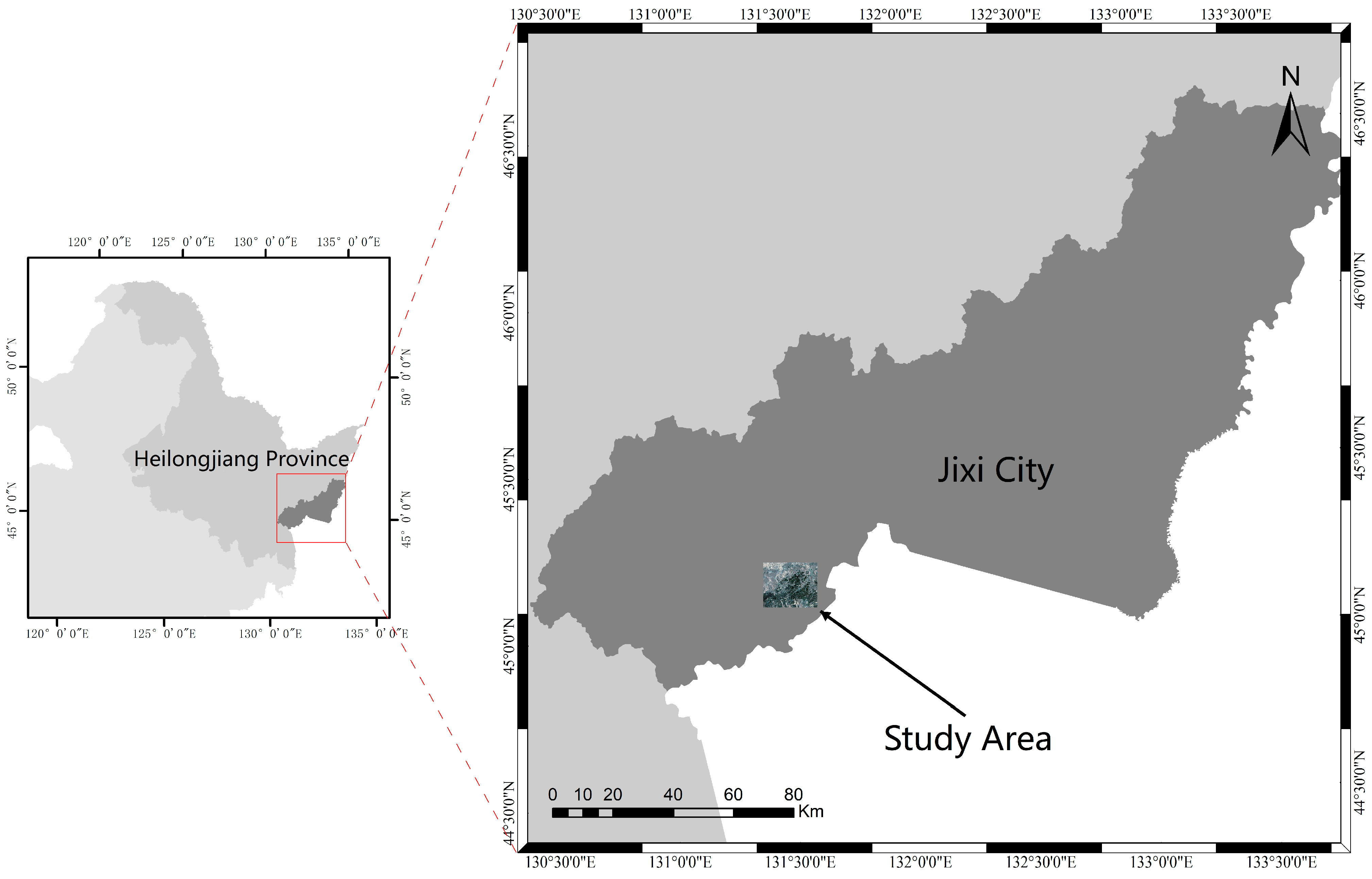
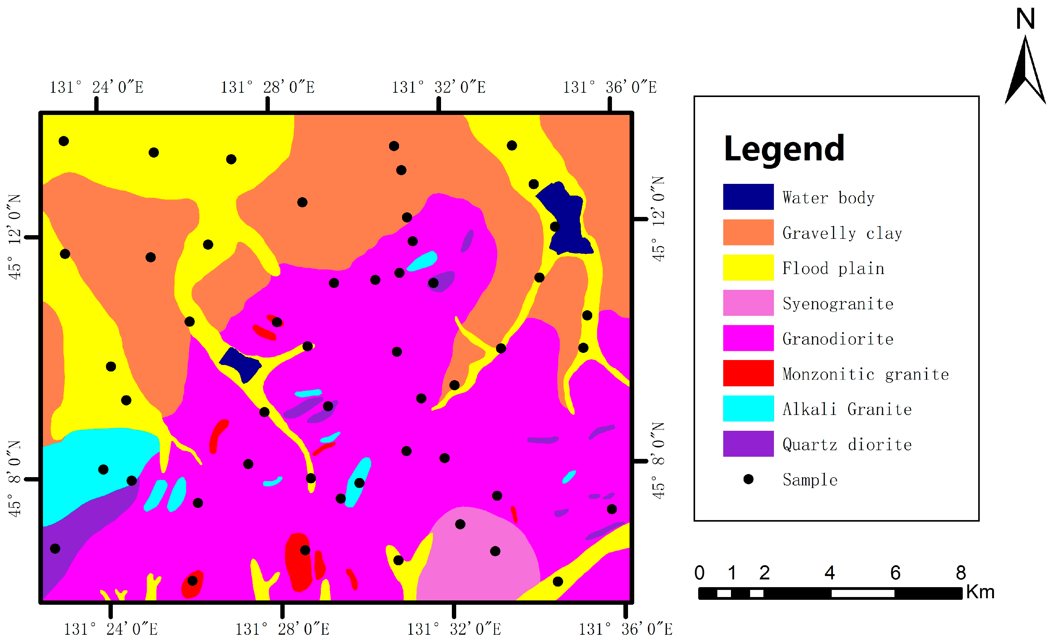
The study area was located in Jixi City, southeastern Heilongjiang Province, China, as shown in Figure 1. Jixi City is connected to Shuangyashan City and Qitaihe City in the north, Russia in the east and south, and Mudanjiang City in the southwest. The geomorphology of Jixi City primarily consists of the Songnen Plain, hills, low mountains, and some mountainous areas. The Songnen Plain is the dominant landform in the region, with relatively flat terrain. The area belongs to the temperate zone, with a monsoon climate characterized by short and warm summers and long and cold winters. Precipitation is concentrated in the summer, and the average annual rainfall is abundant. The vegetation types in the area mainly include coniferous forests, broad-leaved forests, grasslands, and wetlands [30]. The northwestern, northern, and northeastern regions of the study area are primarily characterized by sediments, including gravel, sand, silt, and clay. In the remaining areas, igneous rocks, such as Syenogranite and Granodiorite, predominate.
The geological map shown in Figure 2 was generated through multiple steps. Firstly, field investigations were conducted in the study area to collect preliminary geological information. Secondly, the obtained field data were integrated and supplemented with existing geological maps and remote sensing data. Lastly, the integrated data were digitized and processed using a geographic information system (GIS) to generate the geological map with a scale of 1:250,000. The samples used in this study were derived from the results of the field investigations.

2.2. Data and Data Preprocessing

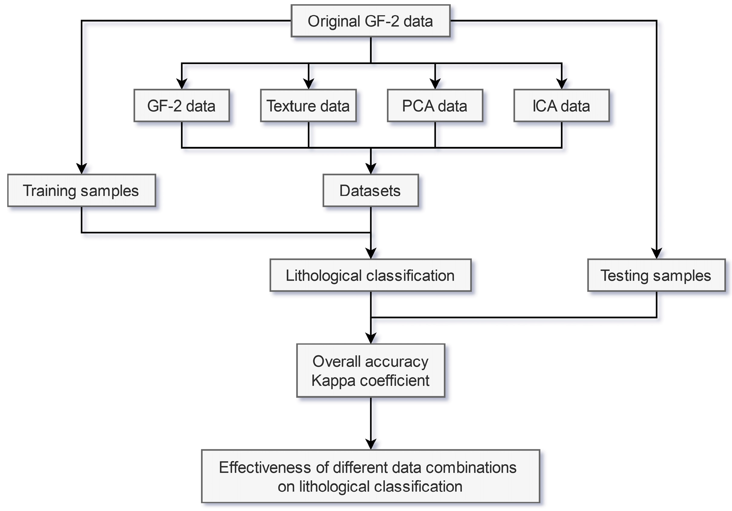
GF-2 image data consist of one panchromatic band and four multispectral bands [31], with spectral characteristics shown in Table 1. The GF-2 image data used in this study were acquired on 25 October 2020 and projected using the Universal Transverse Mercator (WGS 1984 datum, Zone 52N). The multispectral images were radiometrically calibrated, followed by atmospheric correction and orthorectification. The panchromatic image was also radiometrically calibrated and orthorectified. The nearest neighbor diffusion (NNDiffuse) pan sharpening algorithm was used to fuse the calibrated multispectral images with the panchromatic image, which was recently proposed by the Rochester Institute of Technology (RIT) with a suitable image fusion effect [29]. The fused images were then resampled to a 15 m resolution and cropped to obtain a study area of 1000 rows and 1200 columns. All these preprocessing steps were performed in ENVI 5.3 software. Figure 3 shows the flow chart of the lithological classification process.

2.3. Training and Testing Samples

The careful selection of training and testing samples was conducted utilizing the geological map shown in Figure 2 and field survey samples, in combination with visual interpretation. A total of 10 classes were chosen, as presented in Table 2. To minimize the possibility of overfitting, the training samples for each class were ensured to be at least several times the number of data layers to be used for classification.

2.4. Lithological Classification Methods

Four methods were used for lithological classification in this study, including minimum distance classification, maximum likelihood classification, neural network classification, and support vector machine classification. All these four methods were implemented in ENVI 5.3 software, and a brief introduction to these four algorithms is provided below.

2.4.1. Minimum Distance Classification

Minimum distance classification is the most basic classification method and assigns an unknown pixel to the class with the smallest Euclidean distance to it [6,32].

2.4.2. Maximum Likelihood Classification

Maximum likelihood classification is one of the most commonly used supervised classification methods in remote sensing. It uses statistical analysis to calculate probability density functions and assigns an unknown pixel to the class with the highest probability [33,34].

2.4.3. Neural Network Classification

Neural network classification is one of the mainstream machine learning methods and establishes a model by simulating the way the human neural system recognizes and learns [35]. This neural network model consists of many nodes, which are connected by weighted connections and adjust the weights continuously during the training process until the best output is obtained.

2.4.4. Support Vector Machine Classification

Support vector machine classification is one of the most widely used machine learning methods. It maximizes the margin between classes by seeking an optimal separating hyperplane [36,37]. Soft margin techniques and penalty parameters are introduced to improve the generalization ability when the data contain outliers and classes are not linearly separable [22].

2.5. Texture Analysis Methods

Texture is an important feature for identifying image classes [38,39], and there are many methods for defining texture. Among them, the gray-level co-occurrence matrix (GLCM) has been proven to be effective in rock texture analysis [40]. The principle of GLCM is to quantize the gray levels of the original grayscale matrix, establish a GLCM based on the frequency of specific pixel pairs, and calculate different indicators based on the GLCM [41,42,43]. This paper uses 8 different GLCM indicators, which are briefly introduced below (where g (i,j) is the normalized value of the frequency of pixel pair (i,j) and μ and σ2 are the mean and variance of the GLCM, respectively).

2.5.1. Contrast

The Contrast index is used to measure the drastic changes in image grayscale. The clearer and finer the texture of an image, the higher the Contrast value.
The Contrast index provides information about the brightness contrast in rock textures. The Contrast index is of significant importance in describing the details, edges, and variability of rock textures.
The Contrast index measures the degree of difference between adjacent gray-level pixels in rock textures. It helps us understand the contrast and texture variation between gray-level pixels in rock textures. A higher Contrast value indicates a greater difference between adjacent gray-level pixels and a more noticeable texture variation in the rock texture. Conversely, a lower Contrast value indicates relatively similar adjacent gray-level pixels and a smaller texture variation in the rock texture.
In rock texture analysis, the Contrast index can be used to assess the texture variation and edge features of rock textures. Different types of rocks or textures often exhibit different texture features, which are reflected in different Contrast values in terms of the contrast and texture variation between gray-level pixels. Rock textures with complex texture variations and rich edges tend to have higher Contrast values, while relatively uniform and smooth rock textures exhibit lower Contrast values.
The corresponding Contrast data are obtained through calculations using GF-2 data. In subsequent research, the Contrast data will be combined with other data to explore the contribution of this texture index to lithological classification.
C o n t r a s t = j i j 2 g i , j

2.5.2. Correlation

The Correlation index is used to measure the linear correlation of image grayscale. The higher the linear correlation between the grayscale levels of adjacent pixels in an image, the larger the Correlation value.
The Correlation index provides information about the correlation of grayscale values between pixels in rock textures. The Correlation index is highly useful for describing the linearity, directionality, and regularity of rock textures.
The Correlation index measures the linear correlation of pixel values in rock textures. It helps us understand the linear relationship between different grayscale-level pixels in rock textures. A Correlation value closer to 1 indicates a strong linear correlation between pixel values in the rock texture, suggesting a tendency toward a regular and orderly texture. Conversely, a Correlation value closer to 0 indicates less correlation between pixel values in the rock texture, suggesting a tendency toward randomness and disorder in the texture.
In rock texture analysis, the Correlation index can be used to assess the directionality of rock textures. Different types of rocks often exhibit different degrees of linearity and regularity, which are reflected in different correlation characteristics of their texture features. A higher Correlation value implies the presence of significant directional features in the rock texture, while a lower Correlation value indicates a weaker directionality. Directionality is an important distinguishing factor for certain types of rocks.
The corresponding Correlation data are obtained through calculations using GF-2 data. In subsequent research, the Correlation data will be combined with other data to explore the contribution of this texture index to lithological classification.
C o r r e l a t i o n = j ( i μ ) ( j μ ) g i , j σ 2

2.5.3. Dissimilarity

The Dissimilarity index is used to measure the changes in image grayscale, similar to Contrast, but with a difference in that exponential weighting is used in Contrast, whereas linear weighting is used in Dissimilarity.
The Dissimilarity index provides information about the degree of difference between pixels of different grayscale levels in rock textures. The Dissimilarity index is highly useful for describing the level of variation, roughness, and granularity of rock textures.
The Dissimilarity index measures the degree of difference between pixels of different grayscale levels in rock textures. It helps us understand the level of variation between pixels of different grayscale levels in rock textures, i.e., the differences in pixel values. A higher Dissimilarity value indicates a greater difference between different regions in the rock texture, suggesting a tendency toward roughness and granularity. Conversely, a lower Dissimilarity value indicates less difference between different regions in the rock texture, suggesting a tendency toward uniformity and smoothness.
In rock texture analysis, the Dissimilarity index can be used to identify different types of rock textures. Different rock types often exhibit different levels of variation and granularity, which are reflected in different characteristics of their texture features. Rough rock textures tend to have higher Dissimilarity values, indicating larger differences in pixel values within the texture. On the other hand, smooth rock textures exhibit lower Dissimilarity values, indicating relatively smaller differences in pixel values within the texture.
The corresponding Dissimilarity data are obtained through calculations using GF-2 data. In subsequent research, the Dissimilarity data will be combined with other data to explore the contribution of this texture index to lithological classification.
D i s s i m i l a r i t y = j i j g , j

2.5.4. Entropy

The Entropy index is used to measure the disorderliness of image grayscale. The more disorderly and complex the grayscale distribution of an image, the higher the Entropy value. When the values in the GLCM are uniformly distributed, the Entropy value is higher.
The Entropy index provides information about the complexity, uncertainty, and information content in rock textures. The Entropy index is highly useful for describing the texture richness, variation, and level of detail in rock textures.
The Entropy index measures the degree of chaos in the distribution of grayscale levels in rock textures. It helps us understand the uncertainty and complexity of the texture in rock textures. A higher Entropy value indicates a more uniform and complex distribution of grayscale levels in the rock texture, suggesting a tendency toward richness and variation in the texture. Conversely, a lower Entropy value indicates a more concentrated distribution of grayscale levels in the rock texture, suggesting a tendency toward simplicity and uniformity.
In rock texture analysis, the Entropy index can be used to evaluate the level of detail in rock textures. Different rock types often exhibit different levels of complexity and texture richness, which are reflected in different degrees of uncertainty in the distribution of grayscale levels. Rock textures with abundant details tend to have higher Entropy values, indicating a more complex distribution of grayscale levels. On the other hand, rocks with simpler textures exhibit lower Entropy values, indicating a relatively concentrated distribution of grayscale levels.
The corresponding Entropy data are obtained through calculations using GF-2 data. In subsequent research, the Entropy data will be combined with other data to explore the contribution of this texture index to lithological classification.
E n t r o p y = j log g ( i , j ) g , j

2.5.5. Homogeneity

The Homogeneity index, also known as the inverse difference moment, is used to measure the homogeneity of an image. When the grayscale of an image is uniform, Homogeneity value is at its maximum.
The Homogeneity index provides information about the similarity and consistency between pixels of different grayscale levels in rock textures. The Homogeneity index is highly useful for describing the uniformity, smoothness, and proximity between pixels in rock textures.
The Homogeneity index measures the degree of proximity between pixels of different grayscale levels in rock textures. It helps us understand the similarity and consistency between adjacent grayscale-level pixels in rock textures. A higher Homogeneity value indicates smaller differences in grayscale between adjacent pixels in the rock texture, suggesting a tendency toward uniformity and smoothness in the texture. Conversely, a lower Homogeneity value indicates larger differences in grayscale between adjacent pixels in the rock texture, suggesting a tendency toward non-uniformity and roughness in the texture.
In rock texture analysis, the Homogeneity index can be used to evaluate the roughness and granularity of rock textures. Different rock types often exhibit different levels of uniformity and smoothness, which are reflected in different characteristics of grayscale differences between adjacent pixels. Rough rock textures tend to have lower Homogeneity values, indicating larger differences in grayscale between adjacent pixels. On the other hand, smooth rock textures exhibit higher Homogeneity values, indicating relatively smaller differences in grayscale between adjacent pixels.
The corresponding Homogeneity data are obtained through calculations using GF-2 data. In subsequent research, the Homogeneity data will be combined with other data to explore the contribution of this texture index to lithological classification.
H o m o g e n e i t y = j g , j 1 + i j 2

2.5.6. Mean

The Mean index is used to measure the average grayscale of an image.
The Mean index provides information about the average grayscale value in rock textures. The Mean index is highly useful for describing the brightness and grayscale distribution in rock textures.
The Mean index measures the average value of grayscale levels in rock textures. It helps us understand the overall brightness of grayscale levels in rock textures. The Mean value reflects the central position of the pixel grayscale distribution in the rock texture. A higher Mean value indicates a higher overall brightness, while a lower Mean value indicates a lower overall brightness.
In rock texture analysis, the Mean index can be used to evaluate the brightness level of rock textures. Different rock types often exhibit different brightness and grayscale distribution characteristics. Rock textures with higher brightness tend to have higher Mean values, while rock textures with lower brightness exhibit lower Mean values.
Furthermore, it is important to note that the Mean index can only provide overall brightness information about grayscale levels in rock textures and cannot provide detailed information about the distribution range or shape of grayscale levels. Therefore, in rock texture analysis, it is common to combine other GLCM indices or image processing methods for comprehensive analysis.
The corresponding Mean data are obtained through calculations using GF-2 data. In subsequent research, the Mean data will be combined with other data to explore the contribution of this texture index to lithological classification.
M e a n = j i g , j

2.5.7. Second Moment

The Second Moment index is used to measure the regularity of grayscale distribution in an image. Second Moment is negatively correlated with Entropy, and the more uniform and regular the texture of an image, the higher the value of Second Moment. When the values of GLCM are uniformly distributed, the Second Moment value is lower.
The Second Moment index provides information about the uniformity of grayscale-level pixel distribution and texture details in rock textures. The Second Moment index is highly useful for describing the uniformity, level of detail, and smoothness of rock textures.
The Second Moment index measures the uniformity of grayscale-level pixel distribution or the smoothness of texture in rock textures. It helps us understand the overall distribution characteristics of grayscale-level pixels in rock textures. A higher Second Moment value indicates a more uniform distribution of grayscale-level pixels in the rock texture, indicating a tendency toward smoothness in the texture. Conversely, a lower Second Moment value suggests an uneven distribution of grayscale-level pixels in the rock texture, indicating a tendency toward roughness and potentially more texture details and variations.
In rock texture analysis, the Second Moment index can be used to evaluate the level of detail and variability in rock textures. Different rock types or texture types often exhibit different texture characteristics, which are reflected in the energy or Second Moment values of grayscale-level distributions and texture details. Rock textures with rich details and high variability tend to have lower Second Moment values, while relatively uniform and smooth rock textures exhibit higher Second Moment values.
The corresponding Second Moment data are obtained through calculations using GF-2 data. In subsequent research, the Second Moment data will be combined with other data to explore the contribution of this texture index to lithological classification.
S e c o n d   M o m e n t = j g 2 , j

2.5.8. Variance

The Variance index is used to measure the variance of image grayscale. The higher the discreteness of grayscale distribution, the larger the Variance value.
The Variance index provides information about the variability and texture roughness of grayscale-level pixels in rock textures. The Variance index is highly useful for describing the differences, roughness, and dispersion of grayscale-level pixels in rock textures.
The Variance index measures the differences and dispersion of grayscale-level pixels in rock textures. It helps us understand the variability of grayscale-level pixels and the roughness of the texture in rock textures. A higher Variance value indicates greater differences and dispersion of grayscale-level pixels in the rock texture, indicating a rougher texture. Conversely, a lower Variance value suggests a relatively uniform and dense distribution of grayscale-level pixels in the rock texture, indicating smoother texture.
In rock texture analysis, the Variance index can be used to evaluate the roughness and variability of rock textures. Different rock types or texture types often exhibit different detail characteristics, which are reflected in the differences and dispersion of grayscale-level pixels and the resulting Variance values. Rock textures with rougher surfaces and higher variability tend to have higher Variance values, while relatively smooth and consistent rock textures exhibit lower Variance values.
Furthermore, it is important to note that the Variance index can only provide information about the dispersion of grayscale-level pixels in rock textures and cannot provide specific details about grayscale-level distributions and texture morphology. Therefore, in rock texture analysis, it is common to combine other GLCM indices or image processing methods for comprehensive analysis.
The corresponding Variance data are obtained through calculations using GF-2 data. In subsequent research, the Variance data will be combined with other data to explore the contribution of this texture index to lithological classification.
V a r i a n c e = j μ 2 g , j

2.6. Image Processing Methods

This paper employs two image enhancement processing algorithms, namely principal component analysis (PCA) and independent component analysis (ICA). The following provides a brief introduction to these two methods.

2.6.1. Principal Component Analysis

The core idea of PCA is to reduce the complexity of high-dimensional data while preserving the original trends and patterns as much as possible [44,45]. PCA projects the data onto a new principal component space by a linear transformation. From a geometric point of view, the coordinate system of the transformed principal component space rotates at an angle compared to the original coordinate system. The direction of the new axes points toward the direction with large amounts of data information. These axis directions are the principal component directions, which are mutually independent and maintain the same sum of variances before and after transformation. Research shows that PCA has great potential in identifying lithology in multispectral remote sensing images [4,46,47,48].

2.6.2. Independent Component Analysis

Similar to PCA, ICA projects the data onto a new space. However, ICA is based on the non-Gaussian assumption of independent sources. The projected axes are directed toward independent directions, and these independent components provide an approximate estimation of source signals [49]. Statistically speaking, the concept of statistical independence adopted by ICA is stronger than that of uncorrelatedness. Essentially, if two variables are independent, then any value of one variable cannot provide any information about the value of the other variable. If two variables are uncorrelated, however, the value of one variable can provide information about the value of the other variable [50]. Evidence suggests that ICA performs well in feature extraction of remote sensing data [51,52,53,54].

2.7. Data Combination

Eight different texture indices were employed for lithological classification, and different combinations of data were evaluated, as shown in Table 3. Firstly, the GF-2 data were combined with each of the eight different texture indices separately to classify lithology and evaluate the role of different texture indices in lithological classification. Secondly, the eight different texture indices were combined in pairs to obtain 28 different combinations of data. The GF-2 data were combined with these 28 different datasets respectively to classify lithology, and the effects of different combinations were evaluated to identify the better-performing texture indices. Thirdly, various further combinations of data were evaluated based on the results of the first two experiments to assess the effect of different combination methods on lithological classification.
3. Results

This section evaluated the performance of lithological classification using a confusion matrix, with measures such as overall accuracy, Kappa coefficient, producer’s accuracy, and user’s accuracy. Overall accuracy is obtained by dividing the number of correctly classified pixels by the total number of pixels. The Kappa coefficient is a measure of consistency that accounts well for small samples. The producer’s accuracy is the probability of correctly classifying pixels with the true class X, while the user’s accuracy is the probability of pixels classified as X being truly of class X.

3.1. Lithological Classification Based on Different Methods

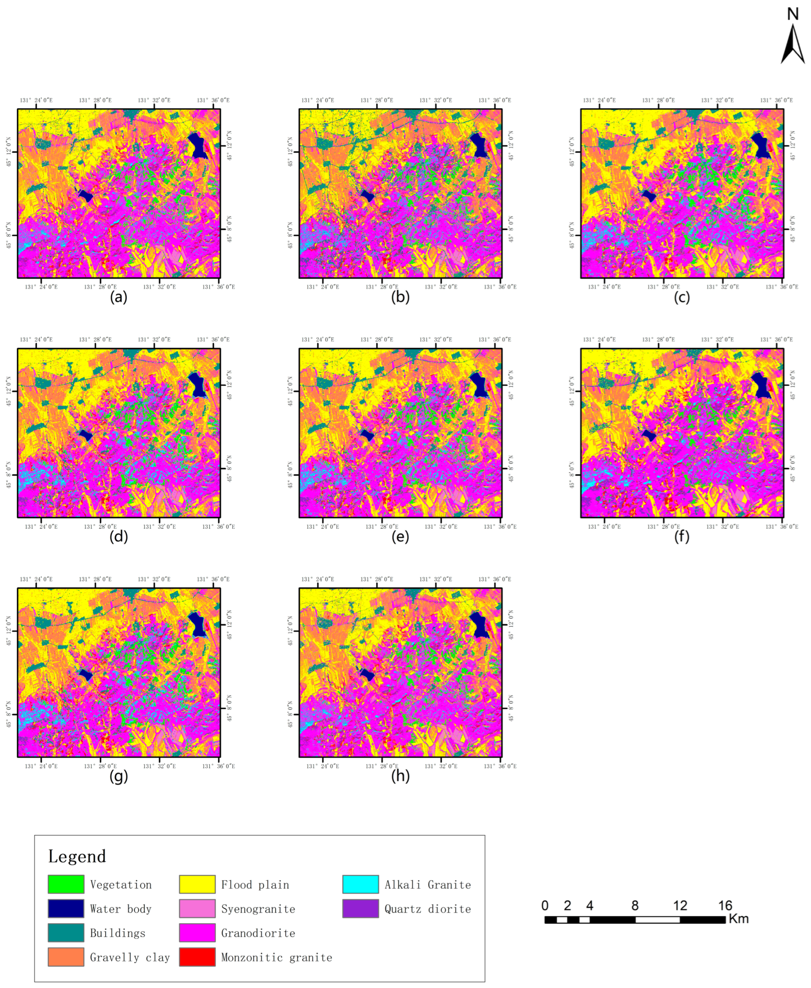
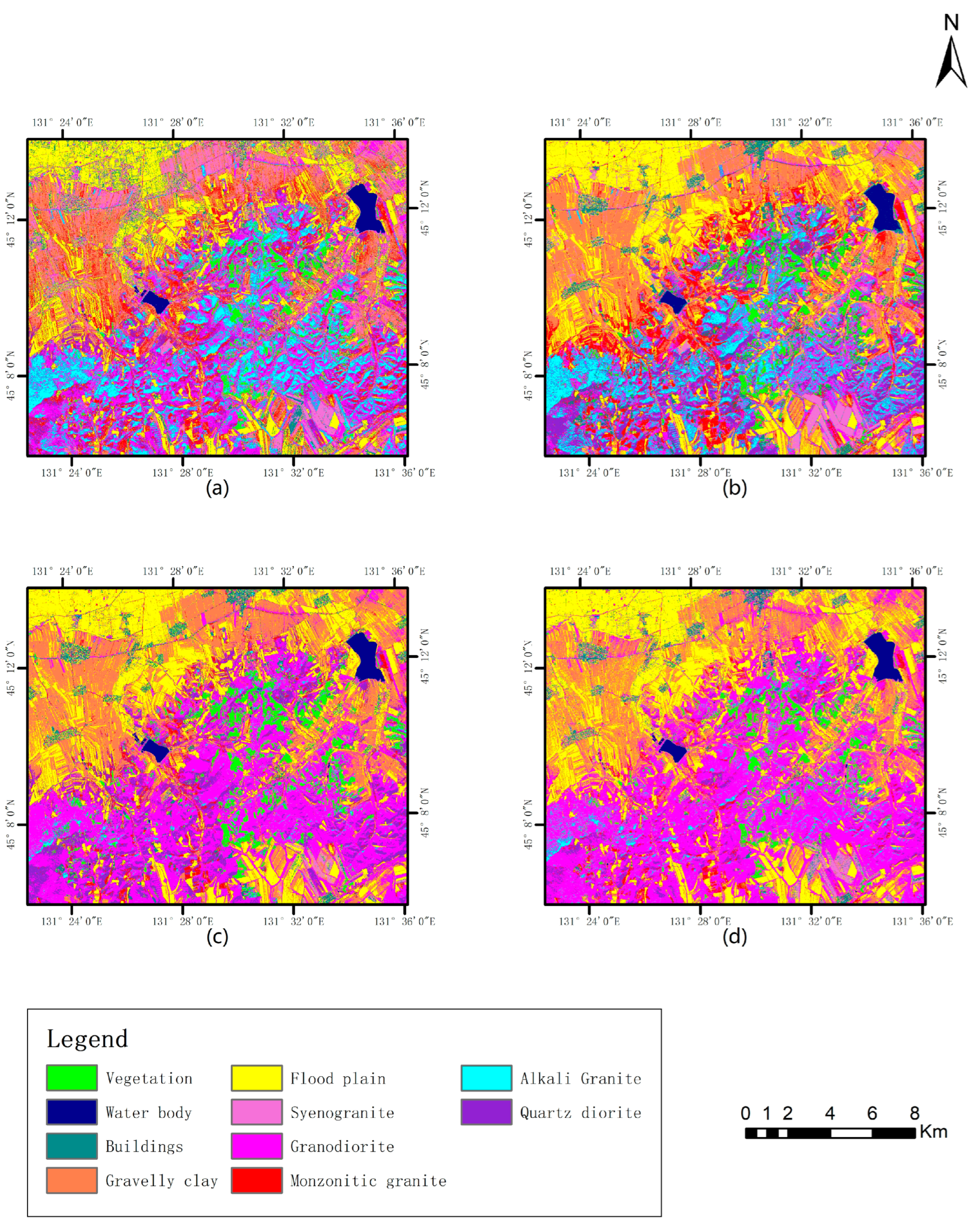
Figure 4 shows the results of lithological classification on GF-2 data using four different methods: minimum distance classification, maximum likelihood classification, neural network classification, and classification. Table 4 presents the overall accuracy and Kappa coefficient obtained using these methods. Results show that the overall accuracy and Kappa coefficient obtained using the minimum distance classification method are the lowest. From the comparison of the four figures, it can be observed that this method poorly separates Buildings, and there are many misclassifications for Gravelly clay and Flood plain, resulting in significant noise. The overall accuracy and Kappa coefficient obtained using the maximum likelihood classification method are better than those obtained using the minimum distance classification. Compared to the minimum distance classification, the maximum likelihood classification significantly improves the classification of Buildings, with many misclassifications corrected and some noise eliminated. However, the maximum likelihood classification method still exhibits noticeable problems of misclassification with Granodiorite and over-classification with Alkali granite. The overall accuracy and Kappa coefficient of neural network classification and support vector machine classification methods are similar and higher than those of the maximum likelihood classification method, indicating their superior classification performance. Due to its slightly higher overall accuracy, we adopted the support vector machine classification method for subsequent studies.

3.2. Lithological Classification Based on Different Texture Features

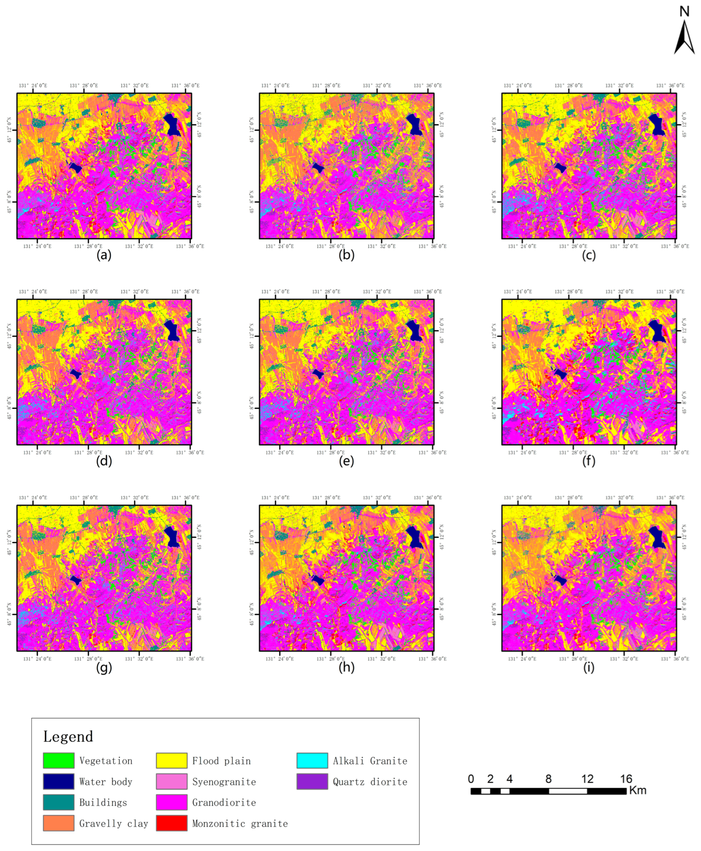
Figure 5 shows the results of lithological classification using the support vector machine classification method on nine different datasets. Table 5 presents the overall accuracy and Kappa coefficient obtained from these nine datasets for comparison. The results indicate that the incorporation of texture features generally improves the classification accuracy compared to using the GF-2 data alone, suggesting the effectiveness of texture features in lithological classification. Among the nine datasets, GF2_D has the highest overall accuracy at 82.5311%, followed by GF2_E (81.5712%), GF2_S (81.3125%), and GF2_M (81.1151%), which all exhibit significant improvements in classification accuracy. GF2_Corr has the lowest overall accuracy of 77.1257% among the eight datasets, including texture features.
Table 6 presents the producer accuracy and user accuracy for each class in the lithological classification of nine datasets. The results indicate that combining the GF2 dataset with texture can improve classification accuracy in most classes, although not all classes show improvements. For instance, in the Granodiorite class, the producer accuracy slightly decreases regardless of the texture combination, suggesting the misclassification of some Granodiorite pixels into other classes. Among these datasets, GF2_D demonstrates higher accuracy in the Buildings, Flood plain, and Syenogranite classes. On the other hand, GF2_M exhibits the most stable performance, with improved accuracy in all classes except for a slight decrease in producer accuracy in the Granodiorite class compared to GF2. GF2_E and GF2_S yield similar results in overall accuracy, Kappa coefficient, and accuracy of individual classes. Although GF2_Corr shows improved accuracy in certain classes compared to GF2, it has the highest number of classes with decreased accuracy compared to other texture-combined datasets.
For the Buildings, Gravelly clay, Flood plain, and Alkali granite classes, combining the GF2 dataset with different textures generally leads to noticeable improvements in both producer and user accuracy. For the Syenogranite, Granodiorite, and Monzonitic granite classes, user accuracy generally improves in different texture-combined datasets, while producer accuracy tends to decrease in most cases. Additionally, except for a slight decrease in user accuracy for the Quartz diorite class in most texture-combined datasets, the user accuracy improves generally for other classes after combining textures.

3.3. Lithological Classification Based on Different Texture Combinations

Table 7 shows the overall accuracy and Kappa coefficient of rock classification based on 28 dual-texture combination datasets. The results indicate that dual-texture overlay generally achieves better classification accuracy than single texture. It is observed that datasets with Mean texture have the highest accuracy ranking, indicating that Mean texture has an advantage in multi-texture overlay. Entropy and Second Moment generally perform well in multiple-texture overlays, consistent with their performance in single-texture analysis. However, the combination of Entropy and Second Moment results in poor performance for the GF2_E_S (81.4555%) dataset, even lower than the GF2_E (81.5712%), indicating that the combination of these two textures does not work well. The combination including Dissimilarity, except with Mean, reduces the accuracy compared to using a single Dissimilarity texture, indicating the poor performance of Dissimilarity in texture combinations. Despite the poor performance of Dissimilarity in texture combinations, its high accuracy in single texture makes the ranking of multi-texture combinations not low.
Contrast, Homogeneity, and Variance textures show poor performance in dual-texture overlays, generally ranking lower, and often even lower than individual texture datasets, such as GF2_H_V, GF2_Con_H, and GF2_S_V. Correlation, although having the worst performance in the single-texture dataset, surprisingly performs well in the dual-texture overlay dataset. Except for the GF2_Corr_D dataset, classification accuracy improves compared to a single texture. Next, we will try to combine more textures and select five textures: Correlation, Dissimilarity, Entropy, Second Moment, and Mean for further research of triple, quadruple, and quintuple texture combinations.
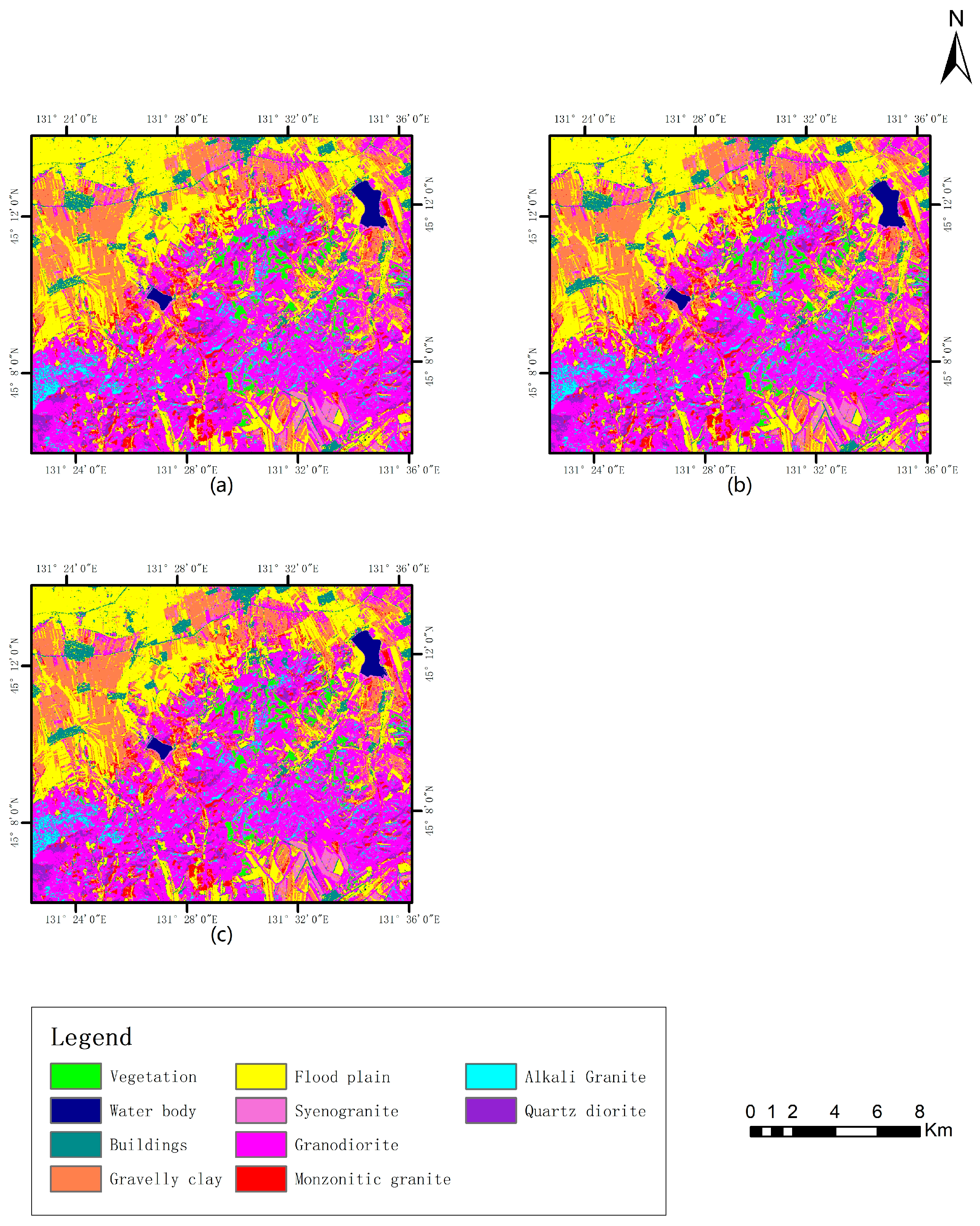
The lithology was classified based on the datasets with triple, quadruple, and quintuple textures obtained from combinations of Correlation, Dissimilarity, Entropy, Second Moment, and Mean using the SVM classification method. Among these datasets, GF2_Corr_E_M, GF2_Corr_D_E_M, and GF2_Corr_D_E_M_S showed the highest accuracy for the triple, quadruple, and quintuple texture datasets, respectively, with their classification results shown in Figure 6. It was observed that the classification results of the three datasets were very similar. Table 8 compares the overall accuracy and Kappa coefficient of the 16 different multiple-texture combination datasets for lithological classification. The results indicated that there was little difference in the accuracy of the datasets with the best performance among the triple, quadruple, and quintuple texture datasets, namely GF2_Corr_E_M (87.8889%), GF2_Corr_D_E_M (88.5220%), and GF2_Corr_D_E_M_S (88.6037%). The dataset with the highest overall accuracy was GF2_Corr_D_E_M_S (88.6037%), which combined all five textures. In addition, the accuracy of the datasets with four textures, such as GF2_Corr_D_M_S (88.4403%), GF2_Corr_E_M_S (88.2157%), and GF2_D_E_M_S (88.0795%), were not significantly different from that of GF2_Corr_D_E_M_S (88.6037%). However, the overall accuracy of the dataset without incorporating the Mean texture, GF2_Corr_D_E_S (82.3678%), was relatively low, indicating that Mean plays a critical role in improving classification accuracy.
Although with an increasing number of layers, the improvement in the highest accuracy gradually becomes weaker, the number of texture overlays seems to be positively correlated with classification accuracy. To verify whether this relationship still exists when more layers are added, we will try to add more layers.
Table 9 compares the overall accuracy and Kappa coefficient of seven different multiple-texture combination datasets for lithological classification. The results indicate that adding more textures does not always lead to better accuracy. Except for the GF2_Corr_D_E_H_M_S (88.6922%) dataset, which had slightly higher accuracy than GF2_Corr_D_E_M_S (88.6037%), the accuracy of the other datasets decreased as more textures were added and was lower than GF2_Corr_D_E_M_S. However, the poor performance of the texture combinations of Contrast, Homogeneity, and Variance themselves may be one of the reasons for the decrease in overall accuracy. Examples of GF2_Con (79.8080%), GF2_V (79.3791%), and GF2_Con_V (79.9033%) show that using the combination of Contrast + Variance produces higher accuracy than using either individually. However, the results of GF2_Con_Corr_D_E_M_S (88.4335%), GF2_Corr_D_E_M_S_V (88.4267%), and GF2_Con_Corr_D_E_M_S_V (88.1544%) indicate that the accuracy after combining Contrast + Variance was lower than using either individually, suggesting that the main reason for the decrease in accuracy was due to stacking too many layers of data. In summary, the number of layers of stacked textures needs to be controlled within a reasonable range, as exceeding this range can result in a decline in performance.

3.4. Lithological Classification Based on PCA and ICA Datasets

PCA and ICA were used to process GF-2 data, resulting in PCA and ICA datasets. The texture combination experiment was conducted using the PCA and ICA datasets as replacements for the original GF-2 data, evaluating the effects of PCA and ICA on lithological classification and the performance of different combination methods.
Figure 7 shows the results of lithological classification using the support vector machine classification method for PCA, ICA, and GF2. Table 10 compares the overall accuracy and Kappa coefficients of lithological classification for the three datasets. The results indicate that, compared to GF2 (74.6681%), both PCA (75.6553%) and ICA (74.7634%) increased the classification accuracy. This suggests that PCA and ICA processing indeed aid lithological classification.
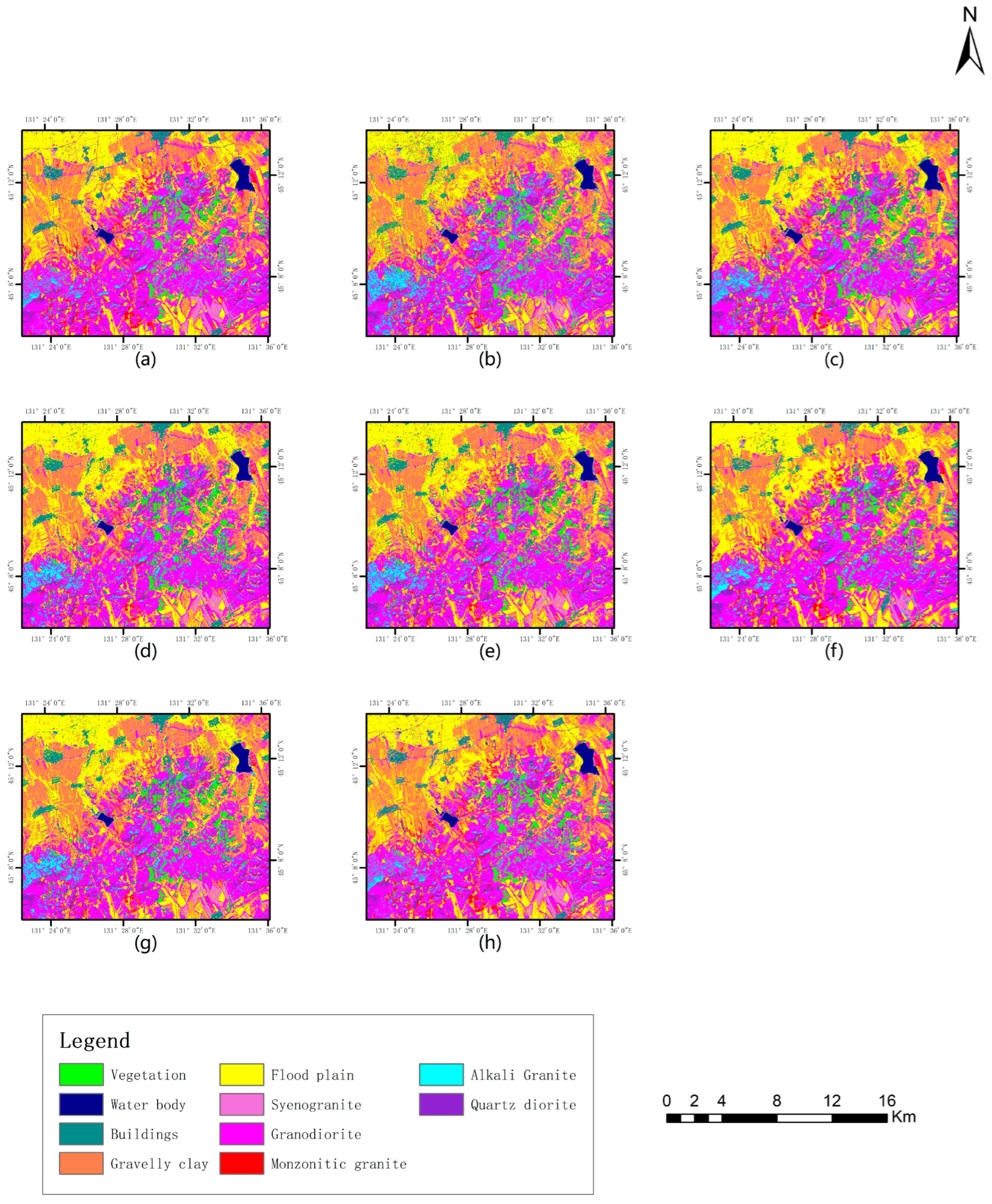
Figure 8 shows the results of lithological classification using the support vector machine classification method for different texture datasets processed by PCA. Figure 9 shows the corresponding results for ICA. Table 11 compares the overall accuracy of lithological classification for different datasets of GF2, PCA, and ICA. The results indicate that when combining textures, the dataset accuracy of both PCA and ICA is higher than that of GF2 with the corresponding textures. Although PCA alone has a higher accuracy (75.6553%) than ICA (74.7634%), when textures are combined, PCA and ICA have their respective strengths. For example, ICA_M (85.0228%) has a higher accuracy than PCA_M (83.0281%). Additionally, unlike GF2_D, which had the highest accuracy among GF2’s texture combinations, PCA_E and ICA_E had the highest accuracies in their respective texture combinations.
Table 12 compares the overall accuracy of lithological classification for different dual-texture datasets of GF2, PCA, and ICA. Due to the poor performance of Contrast and Variance texture combinations, they were not included in this experiment. The results show that the datasets of both PCA and ICA perform better than that of GF2, with PCA_E_M (90.6120%) having the highest accuracy among all 45 datasets. Generally, dataset performance was slightly better for PCA than ICA, particularly for high-accuracy combinations such as PCA_E_M (90.6120%). In contrast, the feature of ICA datasets lies in their consistency, as there is not much variation between the performance of different texture combinations.
Figure 10 and Table 13 present a comparison of the overall accuracies for lithological classification using different multiple-texture datasets, including GF2, PCA, and ICA. Undoubtedly, both the PCA and ICA datasets still outperform the GF2 dataset, with the PCA dataset consistently achieving higher overall accuracy compared to the ICA dataset. PCA_Corr_E_M (91.2860%) performs the best among all triple-texture combination datasets, while PCA_Corr_E_M_S (91.4562%) achieves the best performance among all quadruple-texture combination datasets. The slight difference between them indicates that the effect of texture combination on classification accuracy is small after triple combination. However, the accuracy of the quintuple texture combination PCA_Corr_D_E_M_S (91.3813%) decreases instead of increasing compared to PCA_Corr_E_M_S (91.4562%), which suggests that excessive texture combination not only increases computational complexity but also leads to reduced accuracy. Furthermore, the poor performance of Dissimilarity texture in the PCA dataset and the negative impact caused by its combination with other textures are observed. Continuing to combine textures on the basis of the quintuple texture combination will further demonstrate the drawbacks of excessive texture combination.
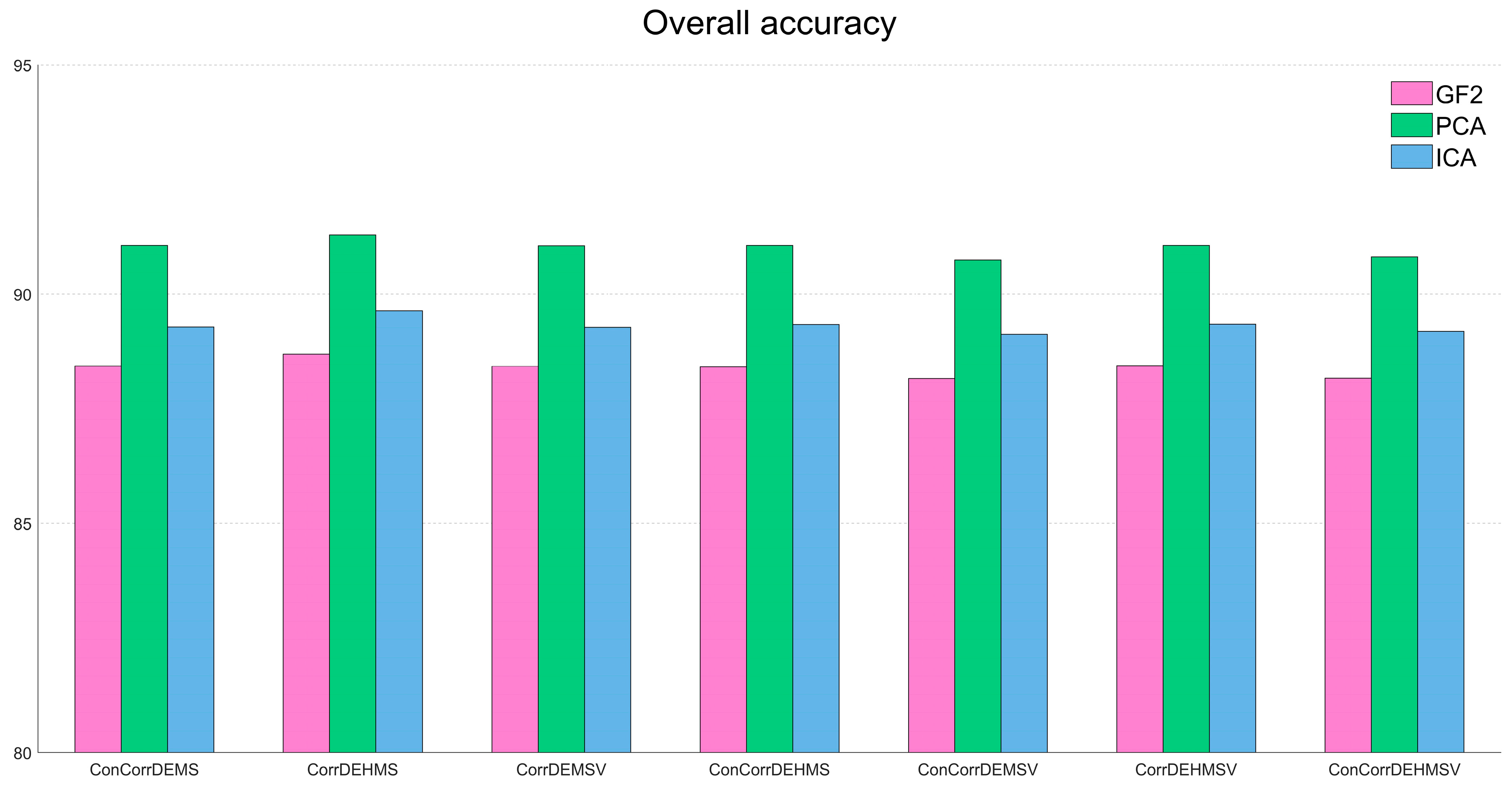
Figure 11 and Table 14 present a comparison of the overall accuracies for lithological classification using different multiple-texture datasets, including GF2, PCA, and ICA. The results demonstrate that the accuracy of various datasets has stabilized after combining multiple textures. All PCA datasets in the table have lower accuracy than the quintuple texture combination PCA_Corr_D_E_M_S (91.3813%) mentioned in previous paragraphs, while the GF2 and ICA datasets, except for GF2_Corr_D_E_H_M_S (88.6922%) and ICA_Corr_D_E_H_M_S (89.6385%), have lower accuracy compared to their corresponding GF2_Corr_D_E_M_S (88.6037%) and ICA_Corr_D_E_M_S (89.5432%). Generally speaking, the number of texture combinations needs to be controlled within a reasonable range.
Table 15 presents the relevant results of the accuracy assessment for the PCA_Corr_E_M dataset mentioned earlier using geological maps. However, the classification accuracy using geological maps is lower compared to using testing samples. This could be attributed to the various limitations associated with digitized geological maps, leading to some uncertainty in the information. In contrast, testing samples provide more accurate information. Furthermore, considering the remote sensing limitations discussed earlier, this level of accuracy is reasonable.

4. Discussion

In this study, different methods were used to classify lithology with GF-2 data, and the results showed that the support vector machine had the highest overall accuracy. Therefore, support vector machine was used for further research.
This study investigates the impact of eight GLCM-defined texture indices on lithological classification. The experimental findings demonstrate the superiority of datasets incorporating arbitrary texture overlays on GF-2 data over those using GF-2 data alone. This suggests a positive influence of all eight texture indices on lithological classification. Notably, the GF2_D dataset exhibited the highest accuracy (82.5311%) due to its sensitivity to grayscale changes. For instance, the Dissimilarity index effectively identifies the Buildings class by leveraging the distinctive grayscale variations associated with artificial structures. Compared to other datasets, GF2_D displayed higher producer and user accuracy for the Buildings class, except for the user accuracy of the GF2_Con dataset. This discrepancy arises from the exponential weighting employed by the Contrast index, making it more responsive to grayscale changes and thereby increasing user accuracy. Nevertheless, excessive sensitivity to grayscale variations can result in subpar classification performance for most classes, thus explaining the relatively low overall accuracy of the GF2_Con dataset.
The Entropy and Second Moment indices serve as complementary measures to assess the regularity of grayscale distribution, albeit from contrasting perspectives. Consequently, GF2_E and GF2_S exhibit consistent overall and individual class accuracy. Among them, GF2_M demonstrates the most stable performance, displaying a stable improvement in classification accuracy across various classes. This stability can be attributed to the smoothing filtering effect of the Mean index, which effectively eliminates noise and yields stable classification enhancement. On the other hand, the Homogeneity and Variance indices reflect grayscale homogeneity and dispersion, respectively. Unlike Entropy, they are not sensitive to grayscale distribution, resulting in the possibility of an image with a high Variance value having a regular grayscale distribution. Experimental results validate the superior classification performance of GF2_E compared to GF2_H and GF2_V. The Correlation index evaluates the linear correlation of grayscale in images, but its direct impact on classification appears to be insignificant, resulting in the poorest performance observed for GF2_Corr.
Considering the distinctive characteristics of each texture index, their combination is expected to enhance classification performance. The research findings demonstrate that dual-texture combinations generally outperform single textures in terms of classification accuracy. Combining the Mean index, which effectively eliminates noise, with other texture indices resulted in higher accuracy datasets. Both the Entropy and Second Moment indices exhibited strong performance in texture combinations, except for the GF2_E_S combination, which suffered from mutual interference stemming from their contrasting perspectives on grayscale distribution.
On the other hand, while the Correlation index did not demonstrate satisfactory performance when used alone, it exhibited suitable results in dual-texture combinations. In contrast, the Dissimilarity index showed excellent performance when used alone, but its effectiveness in dual-texture combinations varied depending on the case. As for the Homogeneity, Variance, and Contrast indices, neither their individual performance nor their performance in combination met the desired standards. Therefore, these three indices were not included in further texture combinations.
Based on the experimental results, incorporating the Mean metric proves essential to enhance classification accuracy. The accuracy of the triple-texture dataset containing Mean exhibits minimal variation, while the accuracy of the quadruple-texture dataset, also including Mean, demonstrates stable performance. When the number of texture combinations is limited to five, there seems to be a positive correlation between the number of combinations and accuracy. However, beyond five combinations, as the number of textures increases, the accuracy of the dataset shows a downward trend. This decline is known as the “curse of dimensionality”, where classification performance initially improves with increasing dimensionality but eventually deteriorates due to overfitting caused by excessive dimensions [55,56]. To mitigate overfitting, increasing the number of training datasets is effective. However, as the dimensionality increases, the required number of training datasets also increases rapidly while the amount of data is limited. Consequently, selecting an appropriate number of layers is crucial in practical classification scenarios.
The paper also explores the impact of PCA and ICA on lithological classification, evaluating their effectiveness in combination with different textures. Experimental findings reveal that datasets combining PCA or ICA with textures achieve higher classification accuracy compared to those combining GF2 with corresponding textures. Among these approaches, PCA displays superior performance in high-accuracy texture combination datasets compared to ICA. ICA has the characteristic that accuracy changes little between various combinations.
Multispectral data are typically collected to acquire spectral information in specific wavelength bands, which reflect the fundamental spectral characteristics of objects on the Earth’s surface. Through the analysis and pattern recognition of spectral information, it is possible to classify and identify different types of rocks. Multispectral sensors are cost-effective and have higher spatial resolution, making data acquisition and processing relatively straightforward. As a result, multispectral data finds wide applications in remote sensing-based lithological classification and has reached a relatively mature stage of development [57,58,59,60,61,62,63,64,65,66]. However, there is still untapped potential for further advancements in the use of multispectral data in lithological classification. With continuous improvements in remote sensing technology and image processing algorithms, the application of multispectral data is becoming more accurate and reliable. For instance, the application of more suitable machine learning methods can enhance the accuracy of lithological classification results. Additionally, combining multispectral data with data processed through different algorithms can further increase the value of multispectral data in lithological classification.
The integration of multispectral data with texture data, PCA data, and ICA data for lithological classification is rare in previous studies. In this research, the combination of multispectral data, texture data, PCA data, and ICA data is explored, and the application value of their integration in lithological classification is investigated. The comprehensive utilization of multiple data sources contributes to improved accuracy and reliability in lithological classification, providing more reliable information support for geological research and resource development. Due to experimental conditions and time limitations, only one study area was selected, and only a subset of texture defined by GLCM was used, which limits the scope of our study.
Despite being in a relatively mature stage of development, there are still new trends emerging in the remote sensing lithological classification of multispectral data. For instance, in the future, we can further integrate data from other sensors, such as radar, to extract additional feature information and enhance the discriminative ability of multispectral data in lithological classification. Additionally, the adoption of high-resolution image decomposition techniques can be employed to decompose and reconstruct multispectral data, aiming to achieve results and accuracy closer to that of hyperspectral data.

5. Conclusions

This study applies a support vector machine to classify lithology in the research area of Jixi City, Heilongjiang Province, China, using GF-2 data. The research aims to evaluate the impact of different texture indices and combinations on lithological classification. Additionally, the effects of combining PCA and ICA with textures on lithological classification were investigated. Based on the experimental results, the following conclusions were drawn:
(1)
In this study, the support vector machine was most suitable for classifying GF-2 data for lithological classification. In addition to this, neural network classification was superior to minimum distance classification and maximum likelihood classification.
(2)
When GF-2 data were combined with single-texture data, the accuracy of datasets combining GF-2 data with any texture generally surpassed that of using GF-2 data alone. Notably, the GF2_D(82.5311%) dataset incorporating the Dissimilarity index achieved the highest overall accuracy, while the GF2_M(81.1151%) dataset employing the Mean index demonstrated stable accuracy improvement for each class.
(3)
The combination of GF-2 data with multiple textures generally resulted in higher classification accuracy compared to using a single texture. The Mean index played a pivotal role in enhancing dataset accuracy. However, excessive texture overlap led to reduced classification accuracy. Considering the performance and limitations of training datasets, utilizing a triple-texture dataset is a reasonable option. In the triple-texture dataset, the GF2_Corr_E_M dataset had the highest accuracy of 87.8889%.
(4)
Both PCA and ICA had a positive effect on the accuracy of lithological classification, with PCA performing better than ICA in high-accuracy texture combination datasets. The accuracy of PCA_Corr_E_M (91.2860%) improved by 3.3971% relative to GF2_Corr_E_M (87.8889%).
Through the integration of multiple data sources, this study holds the potential to enhance the accuracy of lithological classification. Texture data can provide information about the morphological characteristics of rock surfaces, while PCA and ICA can extract the principal and independent components from the original data, further enhancing the feasibility and effectiveness of classification. Lithological classification plays a vital role in geological investigations and resource exploration. By comprehensively utilizing diverse data sources for lithological classification, it can provide more accurate and comprehensive geological information for geological investigations and resource exploration, offering a scientific basis for related decisions.
This article only studied the effects of textures defined by GLCM on lithological classification. In future research, it will be possible to compare the effects of different definitions of texture on lithological classification. Moreover, GF-2 data can be combined with DEM data, gravity-magnetic data, and other multispectral data for further study on the impact of different combinations on lithological classification.

Author Contributions

Conceptualization, T.C. and C.Y.; methodology, T.C. and C.Y.; software, T.C.; validation, T.C.; formal analysis, T.C.; investigation, C.Y.; resources, C.Y. and L.H.; data curation, T.C. and C.Y.; writing—original draft preparation, T.C.; writing—review and editing, T.C., C.Y., L.H., and S.G.; supervision, C.Y. and L.H.; All authors have read and agreed to the published version of the manuscript.

Funding

This research was funded by the Natural Science Foundation of China, grant numbers 42130805 and 42074154, and the China Geological Survey, grant numbers DD20211579.

Data Availability Statement

The GF-2 satellite data were downloaded from the China Centre for Resources Satellite Data and Application (https://data.cresda.cn/#/2dMap (accessed on 25 October 2020)).

Acknowledgments

The authors thank all those students and teachers from Jilin University who actively participated in the field and laboratory work. The authors thank the support of Chunhai Li in editing the paper. The authors thank the China Centre for Resources Satellite Data and Application (https://data.cresda.cn/#/2dMap (accessed on 25 October 2020)) (e-mail: [email protected] and [email protected]) for providing the GF-2 satellite data.

Conflicts of Interest

The authors declare no conflict of interest.

References

  1. Masoumi, F.; Eslamkish, T.; Abkar, A.A.; Honarmand, M.; Harris, J.R. Integration of Spectral, Thermal, and Textural Features of ASTER Data Using Random Forests Classification for Lithological Mapping. J. Afr. Earth Sci. 2017, 129, 445–457. [Google Scholar] [CrossRef]
  2. Alexandridis, T.K.; Topaloglou, C.A.; Lazaridou, E.; Zalidis, G.C. The Performance of Satellite Images in Mapping Aquacultures. Ocean Coast. Manag. 2008, 51, 638–644. [Google Scholar] [CrossRef]
  3. Li, X.; Damen, M.C.J. Coastline Change Detection with Satellite Remote Sensing for Environmental Management of the Pearl River Estuary, China. J. Mar. Syst. 2010, 82, S54–S61. [Google Scholar] [CrossRef]
  4. Amer, R.; Kusky, T.; Ghulam, A. Lithological Mapping in the Central Eastern Desert of Egypt Using ASTER Data. J. Afr. Earth Sci. 2010, 56, 75–82. [Google Scholar] [CrossRef]
  5. Aydal, D.; Arda1, E.; Dumanlilar, Ö. Application of the Crosta Technique for Alteration Mapping of Granitoidic Rocks Using ETM+ Data: Case Study from Eastern Tauride Belt (SE Turkey). Int. J. Remote Sens. 2007, 28, 3895–3913. [Google Scholar] [CrossRef]
  6. Chen, X.; Warner, T.A.; Campagna, D.J. Integrating Visible, near-Infrared and Short-Wave Infrared Hyperspectral and Multispectral Thermal Imagery for Geological Mapping at Cuprite, Nevada. Remote Sens. Environ. 2007, 110, 344–356. [Google Scholar] [CrossRef]
  7. Gad, S.; Kusky, T. Lithological Mapping in the Eastern Desert of Egypt, the Barramiya Area, Using Landsat Thematic Mapper (TM). J. Afr. Earth Sci. 2006, 44, 196–202. [Google Scholar] [CrossRef]
  8. Grebby, S.; Field, E.; Tansey, K. Evaluating the Use of an Object-Based Approach to Lithological Mapping in Vegetated Terrain. Remote Sens. 2016, 8, 843. [Google Scholar] [CrossRef]
  9. Guo, S.; Yang, C.; He, R.; Li, Y. Improvement of Lithological Mapping Using Discrete Wavelet Transformation from Sentinel-1 SAR Data. Remote Sens. 2022, 14, 5824. [Google Scholar] [CrossRef]
  10. Lu, Y.; Yang, C.; Jiang, Q. Evaluation of the Performance of Time-Series Sentinel-1 Data for Discriminating Rock Units. Remote Sens. 2021, 13, 4824. [Google Scholar] [CrossRef]
  11. Ninomiya, Y.; Fu, B.; Cudahy, T.J. Detecting Lithology with Advanced Spaceborne Thermal Emission and Reflection Radiometer (ASTER) Multispectral Thermal Infrared “Radiance-at-Sensor” Data. Remote Sens. Environ. 2005, 99, 127–139. [Google Scholar] [CrossRef]
  12. Pour, A.B.; Hashim, M.; Hong, J.K.; Park, Y. Lithological and Alteration Mineral Mapping in Poorly Exposed Lithologies Using Landsat-8 and ASTER Satellite Data: North-Eastern Graham Land, Antarctic Peninsula. Ore Geol. Rev. 2019, 108, 112–133. [Google Scholar] [CrossRef]
  13. Pour, A.B.; Park, Y.; Park, T.-Y.S.; Hong, J.K.; Hashim, M.; Woo, J.; Ayoobi, I. Evaluation of ICA and CEM Algorithms with Landsat-8/ASTER Data for Geological Mapping in Inaccessible Regions. Geocarto Int. 2019, 34, 785–816. [Google Scholar] [CrossRef]
  14. Rowan, L.C.; Mars, J.C. Lithologic Mapping in the Mountain Pass, California Area Using Advanced Spaceborne Thermal Emission and Reflection Radiometer (ASTER) Data. Remote Sens. Environ. 2003, 84, 350–366. [Google Scholar] [CrossRef]
  15. Hajaj, S.; El Harti, A.; Jellouli, A.; Pour, A.B.; Mnissar Himyari, S.; Hamzaoui, A.; Hashim, M. Evaluating the Performance of Machine Learning and Deep Learning Techniques to HyMap Imagery for Lithological Mapping in a Semi-Arid Region: Case Study from Western Anti-Atlas, Morocco. Minerals 2023, 13, 766. [Google Scholar] [CrossRef]
  16. Karimzadeh, S.; Tangestani, M.H. Evaluating the VNIR-SWIR Datasets of WorldView-3 for Lithological Mapping of a Metamorphic-Igneous Terrain Using Support Vector Machine Algorithm; a Case Study of Central Iran. Adv. Space Res. 2021, 68, 2421–2440. [Google Scholar] [CrossRef]
  17. Shirmard, H.; Farahbakhsh, E.; Müller, R.D.; Chandra, R. A Review of Machine Learning in Processing Remote Sensing Data for Mineral Exploration. Remote Sens. Environ. 2022, 268, 112750. [Google Scholar] [CrossRef]
  18. Sekandari, M.; Masoumi, I.; Pour, A.B.; Muslim, A.M.; Hossain, M.S.; Misra, A. ASTER and WorldView-3 Satellite Data for Mapping Lithology and Alteration Minerals Associated with Pb-Zn Mineralization. Geocarto Int. 2022, 37, 1782–1812. [Google Scholar] [CrossRef]
  19. Zhou, Y.; Zheng, S.; An, Y.; Lai, C. ASTER VNIR-SWIR Based Lithological Mapping of Granitoids in the Western Junggar Orogen (NW Xinjiang): Improved Inputs to Random Forest Method. Earth Space Sci. 2023, 10, 2877. [Google Scholar] [CrossRef]
  20. Harris, J.R.; Rogge, D.; Hitchcock, R.; Ijewliw, O.; Wright, D. Mapping Lithology in Canada’s Arctic: Application of Hyperspectral Data Using the Minimum Noise Fraction Transformation and Matched Filtering. Can. J. Earth Sci. 2005, 42, 2173–2193. [Google Scholar] [CrossRef]
  21. Ge, W.; Cheng, Q.; Jing, L.; Armenakis, C.; Ding, H. Lithological Discrimination Using ASTER and Sentinel-2A in the Shibanjing Ophiolite Complex of Beishan Orogenic in Inner Mongolia, China. Adv. Space Res. 2018, 62, 1702–1716. [Google Scholar] [CrossRef]
  22. Yu, L.; Porwal, A.; Holden, E.-J.; Dentith, M.C. Towards Automatic Lithological Classification from Remote Sensing Data Using Support Vector Machines. Comput. Geosci. 2012, 45, 229–239. [Google Scholar] [CrossRef]
  23. Weszka, J.S.; Dyer, C.R.; Rosenfeld, A. A Comparative Study of Texture Measures for Terrain Classification. IEEE Trans. Syst. Man Cybern. 1976, SMC-6, 269–285. [Google Scholar] [CrossRef]
  24. Conners, R.W.; Harlow, C.A. A Theoretical Comparison of Texture Algorithms. IEEE Trans. Pattern Anal. Mach. Intell. 1980, PAMI-2, 204–222. [Google Scholar] [CrossRef]
  25. Yang, P.; Yang, G. Feature Extraction Using Dual-Tree Complex Wavelet Transform and Gray Level Co-Occurrence Matrix. Neurocomputing 2016, 197, 212–220. [Google Scholar] [CrossRef]
  26. Wang, S.; Xia, Y.; Liu, Q.; Luo, J.; Zhu, Y.; Feng, D.D. Gabor Feature Based Nonlocal Means Filter for Textured Image Denoising. J. Vis. Commun. Image Represent. 2012, 23, 1008–1018. [Google Scholar] [CrossRef]
  27. Rafi, M.; Mukhopadhyay, S. Texture Description Using Multi-Scale Morphological GLCM. Multimed. Tools Appl. 2018, 77, 30505–30532. [Google Scholar] [CrossRef]
  28. Silva, L.E.V.; Duque, J.J.; Felipe, J.C.; Murta Jr, L.O.; Humeau-Heurtier, A. Two-Dimensional Multiscale Entropy Analysis: Applications to Image Texture Evaluation. Signal Process. 2018, 147, 224–232. [Google Scholar] [CrossRef]
  29. Zhang, D.-D.; Xie, F.; Zhang, L. Preprocessing and Fusion Analysis of GF-2 Satellite Remote-Sensed Spatial Data. In Proceedings of the 2018 International Conference on Information Systems and Computer Aided Education (ICISCAE), Changchun, China, 6–8 July 2018; pp. 24–29. [Google Scholar]
  30. Cao, J.; Deng, Z.; Li, W.; Hu, Y. Remote Sensing Inversion and Spatial Variation of Land Surface Temperature over Mining Areas of Jixi, Heilongjiang, China. PeerJ 2020, 8, e10257. [Google Scholar] [CrossRef]
  31. Zheng, Y.; Dai, Q.; Tu, Z.; Wang, L. Guided Image Filtering-Based Pan-Sharpening Method: A Case Study of GaoFen-2 Imagery. ISPRS Int. J. Geo-Inf. 2017, 6, 404. [Google Scholar] [CrossRef]
  32. Jia, K.; Liu, J.; Tu, Y.; Li, Q.; Sun, Z.; Wei, X.; Yao, Y.; Zhang, X. Land Use and Land Cover Classification Using Chinese GF-2 Multispectral Data in a Region of the North China Plain. Front. Earth Sci. 2019, 13, 327–335. [Google Scholar] [CrossRef]
  33. Sun, J.; Yang, J.; Zhang, C.; Yun, W.; Qu, J. Automatic Remotely Sensed Image Classification in a Grid Environment Based on the Maximum Likelihood Method. Math. Comput. Model. 2013, 58, 573–581. [Google Scholar] [CrossRef]
  34. Liu, K.; Shi, W.; Zhang, H. A Fuzzy Topology-Based Maximum Likelihood Classification. ISPRS J. Photogramm. Remote Sens. 2011, 66, 103–114. [Google Scholar] [CrossRef]
  35. Cracknell, M.J.; Reading, A.M. Geological Mapping Using Remote Sensing Data: A Comparison of Five Machine Learning Algorithms, Their Response to Variations in the Spatial Distribution of Training Data and the Use of Explicit Spatial Information. Comput. Geosci. 2014, 63, 22–33. [Google Scholar] [CrossRef]
  36. Awad, M.; Khanna, R. Support Vector Machines for Classification. In Efficient Learning Machines; Apress: Berkeley, CA, USA, 2015; pp. 39–66. [Google Scholar]
  37. Mountrakis, G.; Im, J.; Ogole, C. Support Vector Machines in Remote Sensing: A Review. ISPRS J. Photogramm. Remote Sens. 2011, 66, 247–259. [Google Scholar] [CrossRef]
  38. Haralick, R.M.; Shanmugam, K.; Dinstein, I. Textural Features for Image Classification. IEEE Trans. Syst. Man Cybern. 1973, SMC-3, 610–621. [Google Scholar] [CrossRef]
  39. Julesz, B. Visual Pattern Discrimination. IRE Trans. Inf. Theory 1962, 8, 84–92. [Google Scholar] [CrossRef]
  40. Lobos, R.; Silva, J.F.; Ortiz, J.M.; Díaz, G.; Egaña, A. Analysis and Classification of Natural Rock Textures Based on New Transform-Based Features. Math. Geosci. 2016, 48, 835–870. [Google Scholar] [CrossRef]
  41. Park, Y.; Guldmann, J.-M. Measuring Continuous Landscape Patterns with Gray-Level Co-Occurrence Matrix (GLCM) Indices: An Alternative to Patch Metrics? Ecol. Indic. 2020, 109, 105802. [Google Scholar] [CrossRef]
  42. Iqbal, N.; Mumtaz, R.; Shafi, U.; Zaidi, S.M.H. Gray Level Co-Occurrence Matrix (GLCM) Texture Based Crop Classification Using Low Altitude Remote Sensing Platforms. PeerJ Comput. Sci. 2021, 7, e536. [Google Scholar] [CrossRef]
  43. Srivastava, D.; Rajitha, B.; Agarwal, S.; Singh, S. Pattern-Based Image Retrieval Using GLCM. Neural Comput. Appl. 2020, 32, 10819–10832. [Google Scholar] [CrossRef]
  44. Lever, J.; Krzywinski, M.; Altman, N. Principal Component Analysis. Nat. Methods 2017, 14, 641–642. [Google Scholar] [CrossRef]
  45. Deng, J.S.; Wang, K.; Deng, Y.H.; Qi, G.J. PCA-based Land-use Change Detection and Analysis Using Multitemporal and Multisensor Satellite Data. Int. J. Remote Sens. 2008, 29, 4823–4838. [Google Scholar] [CrossRef]
  46. Pour, A.B.; Park, T.-Y.S.; Park, Y.; Hong, J.K.; Muslim, A.M.; Läufer, A.; Crispini, L.; Pradhan, B.; Zoheir, B.; Rahmani, O.; et al. Landsat-8, Advanced Spaceborne Thermal Emission and Reflection Radiometer, and WorldView-3 Multispectral Satellite Imagery for Prospecting Copper-Gold Mineralization in the Northeastern Inglefield Mobile Belt (IMB), Northwest Greenland. Remote Sens. 2019, 11, 2430. [Google Scholar] [CrossRef]
  47. Amer, R.; Kusky, T.; El Mezayen, A. Remote Sensing Detection of Gold Related Alteration Zones in Um Rus Area, Central Eastern Desert of Egypt. Adv. Space Res. 2012, 49, 121–134. [Google Scholar] [CrossRef]
  48. Liu, L.; Zhou, J.; Jiang, D.; Zhuang, D.; Mansaray, L.R.; Zhang, B. Targeting Mineral Resources with Remote Sensing and Field Data in the Xiemisitai Area, West Junggar, Xinjiang, China. Remote Sens. 2013, 5, 3156–3171. [Google Scholar] [CrossRef]
  49. Li, C.-F.; Yin, J.-Y. Variational Bayesian Independent Component Analysis-Support Vector Machine for Remote Sensing Classification. Comput. Electr. Eng. 2013, 39, 717–726. [Google Scholar] [CrossRef]
  50. Stone, J.V. Independent Component Analysis: An Introduction. Trends Cogn. Sci. 2002, 6, 59–64. [Google Scholar] [CrossRef] [PubMed]
  51. Pour, A.B.; Park, T.-Y.S.; Park, Y.; Hong, J.K.; Zoheir, B.; Pradhan, B.; Ayoobi, I.; Hashim, M. Application of Multi-Sensor Satellite Data for Exploration of Zn–Pb Sulfide Mineralization in the Franklinian Basin, North Greenland. Remote Sens. 2018, 10, 1186. [Google Scholar] [CrossRef]
  52. Gholami, R.; Moradzadeh, A.; Yousefi, M. Assessing the Performance of Independent Component Analysis in Remote Sensing Data Processing. J. Indian Soc. Remote Sens. 2012, 40, 577–588. [Google Scholar] [CrossRef]
  53. Liu, L.; Li, C.; Lei, Y.; Yin, J.; Zhao, J. Feature Extraction for Hyperspectral Remote Sensing Image Using Weighted PCA-ICA. Arab. J. Geosci. 2017, 10, 307. [Google Scholar] [CrossRef]
  54. Pour, A.B.; Park, Y.; Crispini, L.; Läufer, A.; Kuk Hong, J.; Park, T.-Y.S.; Zoheir, B.; Pradhan, B.; Muslim, A.M.; Hossain, M.S.; et al. Mapping Listvenite Occurrences in the Damage Zones of Northern Victoria Land, Antarctica Using ASTER Satellite Remote Sensing Data. Remote Sens. 2019, 11, 1408. [Google Scholar] [CrossRef]
  55. Altman, N.; Krzywinski, M. The Curse(s) of Dimensionality. Nat. Methods 2018, 15, 399–400. [Google Scholar] [CrossRef] [PubMed]
  56. Kavzoglu, T.; Tonbul, H.; Yildiz Erdemir, M.; Colkesen, I. Dimensionality Reduction and Classification of Hyperspectral Images Using Object-Based Image Analysis. J. Indian Soc. Remote Sens. 2018, 46, 1297–1306. [Google Scholar] [CrossRef]
  57. Baid, S.; Tabit, A.; Algouti, A.; Algouti, A.; Nafouri, I.; Souddi, S.; Aboulfaraj, A.; Ezzahzi, S.; Elghouat, A. Lithological Discrimination and Mineralogical Mapping Using Landsat-8 OLI and ASTER Remote Sensing Data: Igoudrane Region, Jbel Saghro, Anti Atlas, Morocco. Heliyon 2023, 9, e17363. [Google Scholar] [CrossRef] [PubMed]
  58. Pereira, J.; Pereira, A.J.S.C.; Gil, A.; Mantas, V.M. Lithology Mapping with Satellite Images, Fieldwork-Based Spectral Data, and Machine Learning Algorithms: The Case Study of Beiras Group (Central Portugal). Catena 2023, 220, 106653. [Google Scholar] [CrossRef]
  59. Goodarzi Mehr, S.; Ahadnejad, V.; Abbaspour, R.A.; Hamzeh, M. Using the Mixture-Tuned Matched Filtering Method for Lithological Mapping with Landsat TM5 Images. Int. J. Remote Sens. 2013, 34, 8803–8816. [Google Scholar] [CrossRef]
  60. Xi, Y.; Mohamed Taha, A.M.; Hu, A.; Liu, X. Accuracy Comparison of Various Remote Sensing Data in Lithological Classification Based on Random Forest Algorithm. Geocarto Int. 2022, 37, 14451–14479. [Google Scholar] [CrossRef]
  61. Lin, J.; Wang, R.; Zhao, B.; Cheng, S. A Comprehensive Scheme for Lithological Mapping Using Sentinel-2A and ASTER GDEM in Weathered and Vegetated Coastal Zone, Southern China. Open Geosci. 2019, 11, 982–996. [Google Scholar] [CrossRef]
  62. Kumar, C.; Chatterjee, S.; Oommen, T.; Guha, A.; Mukherjee, A. Multi-Sensor Datasets-Based Optimal Integration of Spectral, Textural, and Morphological Characteristics of Rocks for Lithological Classification Using Machine Learning Models. Geocarto Int. 2022, 37, 6004–6032. [Google Scholar] [CrossRef]
  63. Mars, J.C. Mineral and Lithologic Mapping Capability of Worldview 3 Data at Mountain Pass, California, Using True- and False-Color Composite Images, Band Ratios, and Logical Operator Algorithms. Econ. Geol. 2018, 113, 1587–1601. [Google Scholar] [CrossRef]
  64. Shebl, A.; Csámer, Á. Stacked Vector Multi-Source Lithologic Classification Utilizing Machine Learning Algorithms: Data Potentiality and Dimensionality Monitoring. Remote Sens. Appl. Soc. Environ. 2021, 24, 100643. [Google Scholar] [CrossRef]
  65. Ninomiya, Y.; Fu, B. Regional Lithological Mapping Using ASTER-TIR Data: Case Study for the Tibetan Plateau and the Surrounding Area. Geosci. Switz. 2016, 6, 39. [Google Scholar] [CrossRef]
  66. Wang, Z.; Zuo, R.; Dong, Y. Mapping Himalayan Leucogranites Using a Hybrid Method of Metric Learning and Support Vector Machine. Comput. Geosci. 2020, 138, 104455. [Google Scholar] [CrossRef]
Figure 1. Location map. The study area is located in Jixi City, Heilongjiang Province, China.
Remotesensing 15 04676 g001
Figure 2. Geological map of the study area.
Remotesensing 15 04676 g002
Figure 3. Flow chart of the lithological classification process.
Remotesensing 15 04676 g003
Figure 4. The lithological classification of the GF-2 dataset using different methods. (a) Minimum distance classification; (b) maximum likelihood classification; (c) neural network classification; (d) support vector machine classification.
Remotesensing 15 04676 g004
Figure 5. The lithological classification of nine different datasets. (a) GF2_Con; (b) GF2_Corr; (c) GF2_D; (d) GF2_E; (e) GF2_H; (f) GF2_M; (g) GF2_S; (h) GF2_V; (i) GF2.
Remotesensing 15 04676 g005
Figure 6. The lithological classification of three different datasets. (a) GF2_Corr_E_M; (b) GF2_Corr_D_E_M; (c) GF2_Corr_D_E_M_S.
Remotesensing 15 04676 g006
Figure 7. The lithological classification of different datasets. (a) PCA; (b) ICA; (c) GF2.
Remotesensing 15 04676 g007
Figure 8. The lithological classification of different datasets. (a) PCA_Con; (b) PCA_Corr; (c) PCA_D; (d) PCA_E; (e) PCA_H; (f) PCA_M; (g) PCA_S; (h) PCA_V.
Remotesensing 15 04676 g008
Figure 9. The lithological classification of different datasets. (a) ICA_Con; (b) ICA_Corr; (c) ICA_D; (d) ICA_E; (e) ICA_H; (f) ICA_M; (g) ICA_S; (h) ICA_V.
Remotesensing 15 04676 g009
Figure 10. Overall accuracy of 48 different datasets.
Remotesensing 15 04676 g010
Figure 11. Overall accuracy of 21 different datasets.
Remotesensing 15 04676 g011
Table 1. Spectral characteristics of GaoFen-2 (GF-2) data.
BandsSpectral Range (nm)Spatial Resolution (m)
Pan450–9000.8
Blue450–5203.2
Green520–590
Red630–690
NIR770–890
Table 2. The training and testing samples.
Class NameTraining Sample (Pixels)Testing Sample (Pixels)
Vegetation325344
Water body18881185
Buildings12691583
Gravelly clay17101460
Flood plain33103066
Syenogranite552506
Granodiorite48274520
Monzonitic granite579507
Alkali granite1200869
Quartz diorite896649
Table 3. Datasets for lithological classification.
DatasetAbbreviationNumber of Data Layers
GF-2 + ContrastGF2_Con8
GF-2 + CorrelationGF2_Corr8
GF-2 + DissimilarityGF2_D8
GF-2 + EntropyGF2_E8
GF-2 + HomogeneityGF2_H8
GF-2 + MeanGF2_M8
GF-2 + Second MomentGF2_S8
GF-2 + VarianceGF2_V8
GF-2 + Contrast + CorrelationGF2_Con_Corr12
GF-2 + Contrast + DissimilarityGF2_Con_D12
GF-2 + Contrast + EntropyGF2_Con_E12
GF-2 + Contrast + HomogeneityGF2_Con_H12
GF-2 + Contrast + MeanGF2_Con_M12
GF-2 + Contrast + Second MomentGF2_Con_S12
GF-2 + Contrast + VarianceGF2_Con_V12
GF-2 + Correlation + DissimilarityGF2_Corr_D12
GF-2 + Correlation + EntropyGF2_Corr_E12
GF-2 + Correlation + HomogeneityGF2_Corr_H12
GF-2 + Correlation + MeanGF2_Corr_M12
GF-2 + Correlation + Second MomentGF2_Corr_S12
GF-2 + Correlation + VarianceGF2_Corr_V12
GF-2 + Dissimilarity + EntropyGF2_D_E12
GF-2 + Dissimilarity + HomogeneityGF2_D_H12
GF-2 + Dissimilarity + MeanGF2_D_M12
GF-2 + Dissimilarity + Second MomentGF2_D_S12
GF-2 + Dissimilarity + VarianceGF2_D_V12
GF-2 + Entropy + HomogeneityGF2_E_H12
GF-2 + Entropy + MeanGF2_E_M12
GF-2 + Entropy + Second MomentGF2_E_S12
GF-2 + Entropy + VarianceGF2_E_V12
GF-2 + Homogeneity + MeanGF2_H_M12
GF-2 + Homogeneity + Second MomentGF2_H_S12
GF-2 + Homogeneity + VarianceGF2_H_V12
GF-2 + Mean + Second MomentGF2_M_S12
GF-2 + Mean + VarianceGF2_M_V12
GF-2 + Second Moment + VarianceGF2_S_V12
GF-2 + Correlation + Dissimilarity + EntropyGF2_Corr_D_E16
GF-2 + Correlation + Dissimilarity + MeanGF2_Corr_D_M16
GF-2 + Correlation + Dissimilarity + Second MomentGF2_Corr_D_S16
GF-2 + Correlation + Entropy + MeanGF2_Corr_E_M16
GF-2 + Correlation + Entropy + Second MomentGF2_Corr_E_S16
GF-2 + Correlation + Mean + Second MomentGF2_Corr_M_S16
GF-2 + Dissimilarity + Entropy + MeanGF2_D_E_M16
GF-2 + Dissimilarity + Entropy + Second MomentGF2_D_E_S16
GF-2 + Dissimilarity + Mean + Second MomentGF2_D_M_S16
GF-2 + Entropy + Mean + Second MomentGF2_E_M_S16
GF-2 + Correlation + Dissimilarity + Entropy + MeanGF2_Corr_D_E_M20
GF-2 + Correlation + Dissimilarity + Entropy + Second MomentGF2_Corr_D_E_S20
GF-2 + Correlation + Dissimilarity + Mean + Second MomentGF2_Corr_D_M_S20
GF-2 + Correlation + Entropy + Mean + Second MomentGF2_Corr_E_M_S20
GF-2 + Dissimilarity + Entropy + Mean + Second MomentGF2_D_E_M_S20
GF-2 + Correlation + Dissimilarity + Entropy + Mean + Second MomentGF2_Corr_D_E_M_S24
GF-2 + Contrast + Correlation + Dissimilarity + Entropy + Mean + Second MomentGF2_Con_Corr_D_E_M_S28
GF-2 + Correlation + Dissimilarity + Entropy + Homogeneity + Mean + Second MomentGF2_Corr_D_E_H_M_S28
GF-2 + Correlation + Dissimilarity + Entropy + Mean + Second Moment + VarianceGF2_Corr_D_E_M_S_V28
GF-2 + Contrast + Correlation + Dissimilarity + Entropy + Homogeneity + Mean + Second MomentGF2_Con_Corr_D_E_H_M_S32
GF-2 + Contrast + Correlation + Dissimilarity + Entropy + Mean + Second Moment + VarianceGF2_Con_Corr_D_E_M_S_V32
GF-2 + Correlation + Dissimilarity + Entropy + Homogeneity + Mean + Second Moment + VarianceGF2_Corr_D_E_H_M_S_V32
GF-2 + Contrast + Correlation + Dissimilarity + Entropy + Homogeneity + Mean + Second Moment + VarianceGF2_Con_Corr_D_E_H_M_S_V36
Table 4. The lithological classification accuracies of the GF-2 dataset using different methods.
Classification MethodOverall Accuracy (%)Kappa Coefficient
Minimum distance classification57.3218 0.5075
Maximum likelihood classification68.8066 0.6418
Neural network classification73.2317 0.6750
Support vector machine classification74.6681 0.6869
Table 5. The lithological classification accuracies of nine different datasets.
RankingDatasetOverall Accuracy (%)Kappa Coefficient
1GF2_D82.53110.7861
2GF2_E81.57120.7740
3GF2_S81.3125 0.7711
4GF2_M81.1151 0.7689
5GF2_H80.6045 0.7618
6GF2_Con79.8080 0.7521
7GF2_V79.3791 0.7471
8GF2_Corr77.1257 0.7175
9GF274.6681 0.6869
Table 6. The lithological classification accuracies of nine different datasets for different classes.
Class NameAccuracy (%)GF2_DGF2_EGF2_SGF2_MGF2_HGF2_ConGF2_VGF2_CorrGF2
VegetationProducer accuracy94.7792.15 93.60 95.06 92.15 93.02 93.02 91.28 93.02
User accuracy99.69 100.00 100.00 100.00 100.00 100.00 100.00 99.68 99.69
Water bodyProducer accuracy100.00 99.07 98.99 100.00 99.24 100.00 100.00 100.00 100.00
User accuracy100.00 100.00 99.91 99.16 100.00 99.16 98.91 100.00 94.20
BuildingsProducer accuracy81.30 76.82 75.68 57.61 74.23 76.94 71.95 48.64 37.84
User accuracy91.08 88.76 85.45 86.94 87.17 92.41 89.61 76.39 80.29
Gravelly clayProducer accuracy90.00 93.15 93.08 87.26 92.40 80.96 81.44 94.32 78.49
User accuracy87.83 83.23 83.53 84.93 83.17 80.74 81.83 76.04 74.13
Flood plainProducer accuracy88.39 87.83 86.89 87.44 86.53 80.59 80.53 85.45 81.05
User accuracy82.32 82.28 81.12 85.00 81.03 85.44 85.26 76.36 77.85
SyenograniteProducer accuracy68.77 53.16 53.95 76.09 51.98 79.25 81.03 27.87 63.83
User accuracy95.34 87.06 86.94 61.40 87.96 70.23 68.22 81.03 60.15
GranodioriteProducer accuracy85.40 85.86 85.15 87.94 85.75 88.12 87.65 87.35 88.54
User accuracy78.86 78.26 78.82 78.46 77.32 74.95 74.95 75.76 72.23
Monzonitic graniteProducer accuracy46.55 41.22 42.41 73.77 41.42 62.13 61.93 44.58 54.64
User accuracy73.75 75.72 78.75 73.48 76.92 58.55 58.47 84.96 60.75
Alkali graniteProducer accuracy53.28 51.44 55.47 39.13 50.86 35.33 36.82 41.89 34.41
User accuracy56.81 60.08 61.17 52.88 56.74 54.72 55.56 51.85 49.92
Quartz dioriteProducer accuracy60.71 64.10 63.02 71.19 58.40 52.54 54.24 59.17 51.16
User accuracy67.81 65.72 65.76 74.64 64.46 66.09 63.88 65.53 67.34
Table 7. The lithological classification accuracies of 28 different datasets.
RankingDatasetOverall Accuracy (%)Kappa Coefficient
1GF2_E_M87.17410.8441
2GF2_M_S86.97660.8418
3GF2_D_M86.50690.8357
4GF2_H_M86.34350.8338
5GF2_Corr_M84.34880.8089
6GF2_Con_M83.6000 0.7995
7GF2_M_V83.07580.7930
8GF2_D_V82.27240.7828
9GF2_Con_D82.1431 0.7812
10GF2_Corr_D82.0546 0.7801
11GF2_Corr_E81.9865 0.7791
12GF2_D_S81.91840.7784
13GF2_D_E81.88440.7779
14GF2_Corr_H81.87760.7772
15GF2_E_H81.69380.7756
16GF2_Corr_S81.63250.7748
17GF2_E_S81.45550.7725
18GF2_Con_E81.3602 0.7713
19GF2_D_H81.32620.7708
20GF2_Con_S81.2717 0.7704
21GF2_H_S81.26490.7701
22GF2_E_V81.06750.7676
23GF2_S_V80.82240.7649
24GF2_Con_H80.5909 0.7616
25GF2_H_V80.46840.7602
26GF2_Con_Corr80.2641 0.7569
27GF2_Con_V79.9033 0.7536
28GF2_Corr_V79.63780.7491
Table 8. The lithological classification accuracies of 16 different datasets.
RankingDatasetOverall Accuracy (%)Kappa Coefficient
1GF2_Corr_D_E_M_S88.6037 0.8615
2GF2_Corr_D_E_M88.5220 0.8605
3GF2_Corr_D_M_S88.4403 0.8596
4GF2_Corr_E_M_S88.2157 0.8568
5GF2_D_E_M_S88.0795 0.8552
6GF2_Corr_E_M87.8889 0.8529
7GF2_Corr_M_S87.8685 0.8527
8GF2_D_E_M87.8685 0.8526
9GF2_D_M_S87.7323 0.8510
10GF2_E_M_S87.6438 0.8499
11GF2_Corr_D_M87.0175 0.8419
12GF2_Corr_D_S82.4631 0.7850
13GF2_Corr_D_E_S82.3678 0.7839
14GF2_Corr_D_E82.2793 0.7827
15GF2_D_E_S82.0069 0.7792
16GF2_Corr_E_S81.9525 0.7787
Table 9. The lithological classification accuracies of seven different datasets.
RankingDatasetOverall Accuracy (%)Kappa Coefficient
1GF2_Corr_D_E_H_M_S88.6922 0.8626
2GF2_Corr_D_E_H_M_S_V88.4403 0.8595
3GF2_Con_Corr_D_E_M_S88.4335 0.8594
4GF2_Corr_D_E_M_S_V88.4267 0.8593
5GF2_Con_Corr_D_E_H_M_S88.4131 0.8592
6GF2_Con_Corr_D_E_H_M_S_V88.1612 0.8561
7GF2_Con_Corr_D_E_M_S_V88.1544 0.8560
Table 10. The lithological classification accuracies of different datasets.
Processing MethodOverall Accuracy (%)Kappa Coefficient
PCA75.6553 0.7015
ICA74.7634 0.6891
GF274.6681 0.6869
Table 11. The comparison of lithological classification accuracies of different datasets.
DatasetOverall Accuracy (%)DatasetOverall Accuracy (%)DatasetOverall Accuracy (%)
GF2_Con79.8080 PCA_Con79.9850 ICA_Con79.8693
GF2_Corr77.1257 PCA_Corr80.8632 ICA_Corr81.0130
GF2_D82.5311 PCA_D84.9888 ICA_D85.1113
GF2_E81.5712 PCA_E86.5546 ICA_E85.9419
GF2_H80.6045 PCA_H85.5810 ICA_H84.7369
GF2_M81.1151 PCA_M83.0281 ICA_M85.0228
GF2_S81.3125 PCA_S86.0099 ICA_S85.7649
GF2_V79.3791 PCA_V79.6923 ICA_V80.1620
Table 12. The comparison of lithological classification accuracies of 45 different datasets.
DatasetOverall Accuracy (%)DatasetOverall Accuracy (%)DatasetOverall Accuracy (%)
GF2_Corr_D82.0546 PCA_Corr_D85.7308 ICA_Corr_D86.0372
GF2_Corr_E81.9865 PCA_Corr_E86.8950 ICA_Corr_E86.3912
GF2_Corr_H81.8776 PCA_Corr_H86.6431 ICA_Corr_H85.9078
GF2_Corr_M84.3488 PCA_Corr_M86.7248 ICA_Corr_M85.9010
GF2_Corr_S81.6325 PCA_Corr_S86.7792 ICA_Corr_S86.3095
GF2_D_E81.8844 PCA_D_E86.1801 ICA_D_E86.0916
GF2_D_H81.3262 PCA_D_H85.2747 ICA_D_H84.8322
GF2_D_M86.5069 PCA_D_M88.7943 ICA_D_M88.2157
GF2_D_S81.9184 PCA_D_S85.8057 ICA_D_S86.3163
GF2_E_H81.6938 PCA_E_H86.1938 ICA_E_H86.0440
GF2_E_M87.1741 PCA_E_M90.6120 ICA_E_M88.8216
GF2_E_S81.4555 PCA_E_S86.1189 ICA_E_S85.6015
GF2_H_M86.3435 PCA_H_M89.4887 ICA_H_M88.2225
GF2_H_S81.2649 PCA_H_S85.9078 ICA_H_S86.1189
GF2_M_S86.9766 PCA_M_S90.4691 ICA_M_S88.6786
Table 13. The comparison of lithological classification accuracies of 48 different datasets.
DatasetOverall Accuracy (%)DatasetOverall Accuracy (%)DatasetOverall Accuracy (%)
GF2_Corr_D_E82.2793 PCA_Corr_D_E86.6431 ICA_Corr_D_E87.0515
GF2_Corr_D_M87.0175 PCA_Corr_D_M89.5568 ICA_Corr_D_M88.9577
GF2_Corr_D_S82.4631 PCA_Corr_D_S86.5818 ICA_Corr_D_S87.1060
GF2_Corr_E_M87.8889 PCA_Corr_E_M91.2860 ICA_Corr_E_M89.0394
GF2_Corr_E_S81.9525 PCA_Corr_E_S86.7248 ICA_Corr_E_S87.1060
GF2_Corr_M_S87.8685 PCA_Corr_M_S91.1771 ICA_Corr_M_S89.0666
GF2_D_E_M87.8685 PCA_D_E_M90.5031 ICA_D_E_M89.0666
GF2_D_E_S82.0069 PCA_D_E_S85.6219 ICA_D_E_S86.1052
GF2_D_M_S87.7323 PCA_D_M_S90.4759 ICA_D_M_S89.1279
GF2_E_M_S87.6438 PCA_E_M_S90.9865 ICA_E_M_S88.7603
GF2_Corr_D_E_M88.5220 PCA_Corr_D_E_M91.2043 ICA_Corr_D_E_M89.4683
GF2_Corr_D_E_S82.3678 PCA_Corr_D_E_S86.4184 ICA_Corr_D_E_S87.0583
GF2_Corr_D_M_S88.4403 PCA_Corr_D_M_S91.3473 ICA_Corr_D_M_S89.5977
GF2_Corr_E_M_S88.2157 PCA_Corr_E_M_S91.4562 ICA_Corr_E_M_S89.1347
GF2_D_E_M_S88.0795 PCA_D_E_M_S90.7209 ICA_D_E_M_S88.8692
GF2_Corr_D_E_M_S88.6037 PCA_Corr_D_E_M_S91.3813 ICA_Corr_D_E_M_S89.5432
Table 14. The comparison of lithological classification accuracies of 21 different datasets.
DatasetOverall
Accuracy (%)
DatasetOverall
Accuracy (%)
DatasetOverall
Accuracy (%)
GF2_Con_Corr_D_E_M_S88.4335 PCA_Con_Corr_D_E_M_S91.0613 ICA_Con_Corr_D_E_M_S89.2845
GF2_Corr_D_E_H_M_S88.6922 PCA_Corr_D_E_H_M_S91.2860 ICA_Corr_D_E_H_M_S89.6385
GF2_Corr_D_E_M_S_V88.4267 PCA_Corr_D_E_M_S_V91.0545 ICA_Corr_D_E_M_S_V89.2777
GF2_Con_Corr_D_E_H_M_S88.4131 PCA_Con_Corr_D_E_H_M_S91.0613 ICA_Con_Corr_D_E_H_M_S89.3390
GF2_Con_Corr_D_E_M_S_V88.1544 PCA_Con_Corr_D_E_M_S_V90.7414 ICA_Con_Corr_D_E_M_S_V89.1211
GF2_Corr_D_E_H_M_S_V88.4403 PCA_Corr_D_E_H_M_S_V91.0613 ICA_Corr_D_E_H_M_S_V89.3458
GF2_Con_Corr_D_E_H_M_S_V88.1612 PCA_Con_Corr_D_E_H_M_S_V90.8094 ICA_Con_Corr_D_E_H_M_S_V89.1824
Table 15. The classification accuracies of PCA_Corr_E_M dataset using geological map.
Overall Accuracy (%)56.8237
Kappa coefficient0.4146
Class nameProducer accuracy (%)User accuracy (%)
Water body89.97 98.37
Gravelly clay44.76 62.91
Flood plain70.04 44.90
Syenogranite28.82 45.64
Granodiorite60.84 75.60
Monzonitic granite45.36 14.39
Alkali granite50.08 35.05
Quartz diorite45.53 20.99
Disclaimer/Publisher’s Note: The statements, opinions and data contained in all publications are solely those of the individual author(s) and contributor(s) and not of MDPI and/or the editor(s). MDPI and/or the editor(s) disclaim responsibility for any injury to people or property resulting from any ideas, methods, instructions or products referred to in the content.