1. Introduction
Visual Simultaneous Localization and Mapping (SLAM) is considered to be one of the core technologies for mobile robots. The main task is to simultaneously estimate the trajectory of a mobile robot and reconstruct a map of its surroundings and environment from successive frames. Visual SLAM has attracted much attention in drones and self-driving cars because it has the advantage of low cost and the rich environmental information obtained by using the cameras as sensors. Meanwhile, the trend of multi-sensor information fusion makes IMU (Inertial Measurement Unit) widely combined with cameras in the SLAM system, because they can complement each other [
1]. IMU allows the robot to directly obtain both acceleration and angular velocity information, making the SLAM system more robust even in low-texture environments where tracking by pure vision may fail.
Visual SLAM is generally divided into two main approaches: direct method and feature-based method. Direct methods are used to estimate the camera motion by minimizing the pixel brightness errors between consecutive frames, such as DSO [
2] and SVO [
3]. However, its prerequisite requires the assumption that the local brightness of the sequence is constant, making it sensitive to changes in brightness. In contrast, the feature-based method detects and matches key points between consecutive frames and then minimizes the reprojection errors to simultaneously estimate the poses and construct a map [
4], such as PTAM [
5] and ORB-SLAM2 [
6]. The feature-based method is more robust than the direct method because the discriminative key points are relatively invariant to changes in viewpoint and illumination [
7]. However, the continued expansion of SLAM applications and mobile robots, such as augmented reality and autonomous driving, presents some new challenges, including low-texture or structured engineering environments [
8,
9]. Therefore, extracting key points will become difficult, which can result in degraded performance of the SLAM system and even tracking failure. Fortunately, most low-texture environments, such as white walls and corridors, have more line segment features, although fewer feature points can be extracted. Therefore, more and more SLAM systems with point and line features have been proposed in recent years, such as PL-VIO [
10] and PL-SLAM [
11].
The method based on point and line features greatly enhances the robustness of the SLAM system in low-texture environments. However, it still cannot change the shortcoming of the purely visual SLAM system, which is sensitive to rotation and high speed. For the above issue, a multi-sensor information fusion of IMU and camera is a good strategy. The IMU measurement can provide more precise motion data, while the combination of both can compensate for visual degradation of the camera and correct IMU drift. At present, the most successful systems combining camera and IMU are ORB-SLAM3 [
12] and VINS-Mono [
13]. ORB-SLAM3 integrated IMU on the basis of ORB-SLAM2, which greatly improved the performance of the system. ORB-SLAM3 is one of the most advanced visual-inertial SLAM systems based on the point feature method. Our work is also based on the ORB-SLAM3. The essence of our work is to propose a tightly-coupled visual-inertial SLAM system based on point and line features and to improve Edge Drawing lines (EDlines) [
14] in order to increase the processing speed of the system. The main contributions are as follows:
- (1)
An improved line feature detection method based on EDlines. This method improves the accuracy of the system by detecting the curvature of line segments and improving the selection standard of the minimum line segment length to eliminate line segments that would increase error, while having less processing time.
- (2)
A more advanced experiment-based adapting factor that further balances the error weights of line features based on a combination of the number of interior point matches and the length of the line segment.
- (3)
An autonomously selectable loop detection method for combined point and line features, while having a more advanced similarity score evaluation criterion. The similarity scores of point features and line features are considered both in time and space, while an adaptive weight is used to adapt to texture-varying scenes
- (4)
A tightly-coupled stereo visual-inertial SLAM system with point and line features. Experiments conducted on the EuRoC dataset [
15] and in real environments demonstrate better performance than those SLAM systems based on point and line features or based on point features and IMU.
2. Related Work
In this section, we will discuss point-line SLAM systems and visual inertial SLAM systems. Most of the existing visual-inertial fusion methods can be divided into loosely-coupled and tightly-coupled approaches [
16]. Loosely-coupled approaches separately estimate the IMU data and vision, and then makes a fusion of two results, such as [
17,
18]. The tightly-coupled approach uses IMU and camera together to construct motion and observation equations and then performs state estimation. This method makes the sensors more complementary and can achieve better results through mutual optimization. VINS-Mono [
13] and ORB-SLAM3 [
12] are two of the most well-known open source visual-inertial SLAM systems, on which many studies have improved. ORB-SLAM3 is an improvement on ORB-SLAM2 [
6]. ORB-SLAM3 improved the robustness of the system by integrating IMU, multi-map stitching techniques and achieved the highest accuracy on some public datasets.
Among the related work on SLAM with point and line features, Line Segment Detector (LSD) [
19] is a straight line detection segmentation algorithm, which is widely used in line feature extraction and SLAM systems based on line features because of its ability to control the number of false detections at a low level without parameter adjustment. The core idea is to merge pixel points with similar gradients in the same gradient to achieve the effect of extracting local line features with sub-pixel level accuracy in linear time. The most representative works on the combination of point-line features are PL-SLAM [
20], which used line segment endpoints to represent line features, and the PL-SLAM [
11] of the same name, which is a stereo SLAM system using LSD and a line band descriptor (LBD) method [
21] to match in real time. Regarding point and line matching, PL-SLAM [
11] compared the descriptors of features and the process was only accepted if the candidate was the best mutual match. We also adopt this policy for lines in our work. Another work [
22] used Plücker coordinates and orthogonal representations to derive the Jacobian matrix and construct line feature reprojection errors, which is a great help for bundle adjustment (BA) with points, lines and IMU in the other, later SLAM systems. PL-VIO [
10], based on the VINS-Mono, also used the LSD to extract line segment features and the LBD for line segment matching. At the same time, it added line features to the visual-inertial odometry to achieve a tightly-coupled optimization of point-line features and IMU measurements, which is better than the visual-inertial SLAM systems based only on point features. However, due to the time-consuming process of line feature extraction used to compute the matching, PL-VIO cannot extract and match line features in real time. PL-VINS [
23], on the basis of PL-VIO, achieved real-time operation of the LSD algorithm as much as possible, without affecting the accuracy, by adjusting the implicit parameters of the LSD. PL-VINS realized a real-time visual inertial SLAM system based on point and line features. However, the performance of LSD line detection was still unsatisfactory for real-time applications [
22], so only the point feature was applied in the closed-loop part and the line feature was not fully utilized. In addition, PEI-VINS [
24] applied the EDlines method to reduce the line feature detection time and proved the effectiveness of system. Also based on VINS-Mono is the PLI-VINS [
25], which tightly coupled point features, line features, and IMU, and has been experimentally validated for accurate position evaluation by multi-sensor information fusion.
The classic bundle adjustment (BA) aims to optimize the poses and landmarks, which play an important role in SLAM optimization. Expanded Kalman filtering (EKF) was used in early SLAM optimization, such as MonoSLAM [
26] in 2007. Only in recent years has the nonlinear optimization method BA become popular due to the increase in computational power. In 2007, PTAM [
5] first used the nonlinear optimization method for combined optimization of poses and landmarks, and used the reprojection error of points as a constraint edge for BA, which proved that the nonlinear optimization results were better than those based on filtering. Later, ORB-SLAM2 has a complete realization of constrained edges of points in BA based on the ORB feature [
27], which had a significant effect on the following optimization based on point features. Zuo et al. first used orthogonal representations in SLAM based on line features, and added the complete reprojection error of the line to the constrained edges of BA [
22], which has been followed in point-line SLAM since then. PL-VIO used LSD to combine line features into visual inertial tightly coupled optimization, while using IMU residuals, reprojection errors of point and line, as constraint edges. Then, PL-SLAM [
11] took the distance from the endpoints of the line to the projected straight line as the reprojection error of the line, and fully added the point features and line features to the various parts of the tightly coupled bundle adjustment, which made the bundle adjustment based on the combination of points and lines even better.
Another work that inspired our system is ORB-LINE-SLAM [
28], based on the framework of ORB-SLAM3. ORB-LINE-SLAM added an experimentally tuned adapting factor, which is also used and improved in our system. However, ORB-LINE-SLAM has large biases and even tracking failure in challenging environments, for example, motion blur. Meanwhile, line feature detection with LSD took a lot of time in ORB-LINE-SLAM. According to our experiments, its real-time performance is not ideal. Therefore, we improve EDlines to enhance accuracy and robustness with less processing time than ORB-LINE-SLAM.
3. System Overview
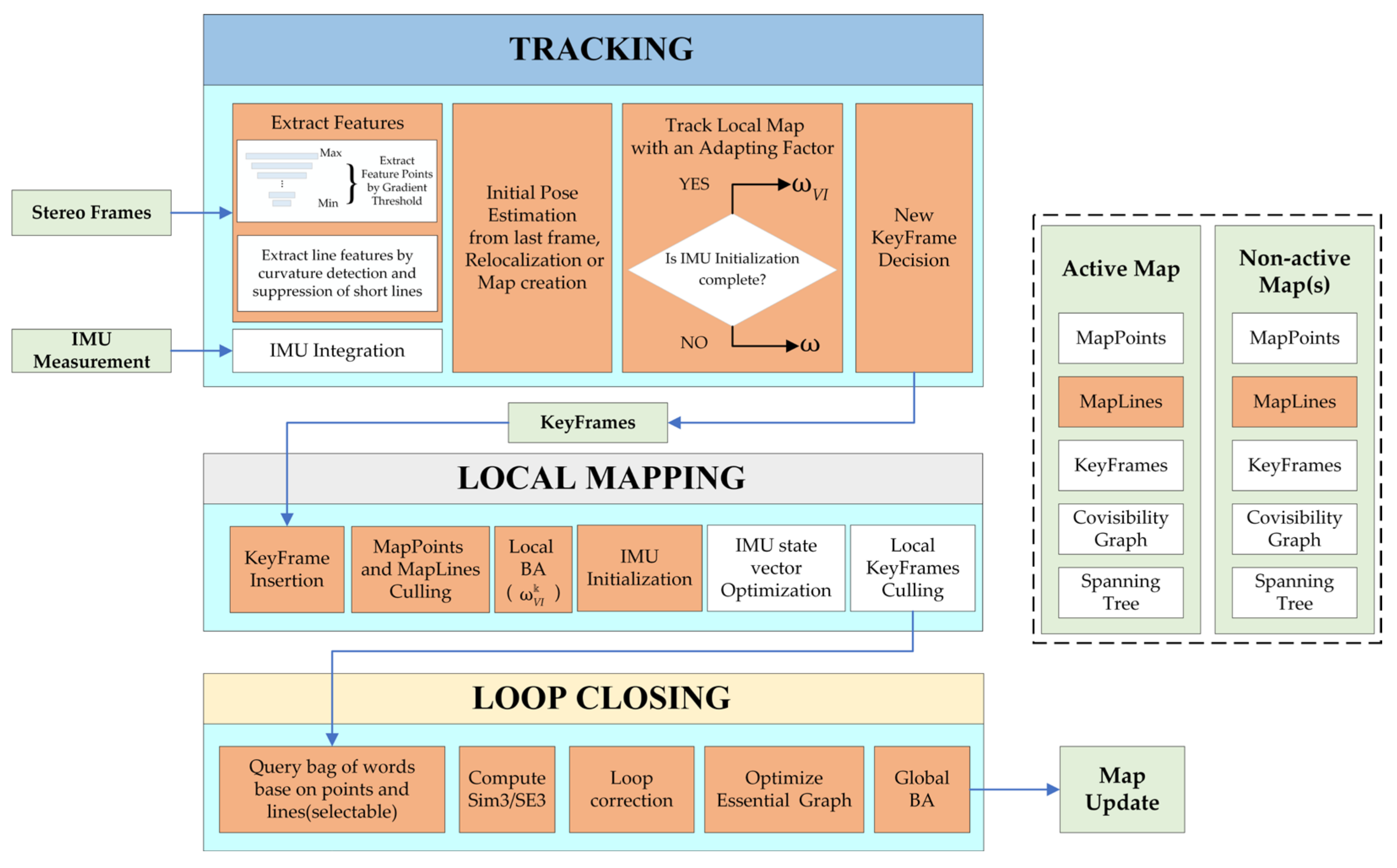
Our method mainly improves on the ORB-SLAM3 and also implements three different threads: tracking, local mapping, and loop closing. We incorporate line features into each module of ORB-SLAM3.
Figure 1 shows the framework of our system, in which the orange-colored part is where we add line features, and the rest is the same as ORB-SLAM3.
3.1. Tracking
The tracking thread calculates the initial pose estimation by minimizing the reprojection error of point and line matches detected between the current frame and the previous frame, and updates the IMU pre-integration from the last frame. A detailed description of pose estimation will be demonstrated in
Section 5. When IMU is initialized, the initial pose will be predicted by IMU. After that, we combine the point and line feature matching and IMU information to jointly optimize the pose of the current frame.
For point features, we use the ORB [
27] (Oriented FAST and Rotated BRIEF) method because of its good performance for key point detection. Its improved “Steer BRIEF” also allows for fast and efficient key point matching. Meanwhile, to accelerate the matching speed and reduce the number of outliers, as with PL-SLAM [
11], we only choose the best match in the left image corresponding to the best match in the right image as the best match pair. The processing of line features will be described in detail in
Section 4.
3.2. Local Mapping
The core idea of this section is divided into two parts. The first is local bundle adjustment based on keyframes, and the second is IMU initialization and state vector optimization.
After inserting the keyframes from the tracking thread, the system will check the new map points and map lines, and then reject the new map points and map lines with bad quality according to observation of them, which will be guided by the following strategy:
- (1)
If the number of frames tracked to the point and line is less than 25% and 20%, respectively, of the number of frames visible in their local map, then delete the map point or map line;
- (2)
if map points and map lines are observed less than three times in three consecutive frames created, then delete them.
As for the initialization of the IMU, we follow the ORB-SLAM3 method [
12] to quickly obtain more accurate IMU parameters. After that, we filter the line segments again according to the update of the IMU gravity direction. When the angle between the gravity direction and the 3D line changes between the current frame and the last keyframe by more than a given threshold, this 3D line will be set as an exception and it will be discarded.
3.3. Loop Closing
Loop closing thread uses a bag of words method which is implemented by DBoW2 [
29], based only on the key points and lines for the loop detection. Then, it performs loop correction or map merge. After that, the system performs a full bundle adjustment (BA) to further optimize the map.
It is worth noting that we provide a loop detection part that can autonomously select whether or not to add line features. According to our experiments, although adding line features in loop detection is beneficial to the accuracy, it will also bring a large computational overhead. This is not conducive to the original intention of real-time SLAM, so we provide a selectable model to balance the accuracy and speed.
3.4. Multi-Map
Our system also includes a multi-map (Atlas) representation, consisting of the currently active map and the inactive map, which consists of the following parts:
4. Tracking
This section introduces the processing methods of point and line features, a two-stage tracking model and an adapting weight factor based on experiment for the reprojection error on the balance line feature. Finally, we propose a new keyframe selection strategy on line features to ensure its effectiveness.
4.1. Feature Selection and Match
4.1.1. Point Features Detection by Gradient Threshold
For the extraction of point features, a fixed extraction threshold is used in the traditional method (ORB-SLAM3), which cannot adapt to the changing environment of texture and easily causes tracking failure. In addition, with the addition of line features to the system, point features are no longer the only source of features, so the use of traditional fixed thresholds to extract point features can also cause redundancy in the system and increase unnecessary computation. Therefore, in order to increase the adaptability of the system to low texture environments while avoiding redundancy, we propose adaptive gradient thresholding to extract point features. The core idea is to predict the threshold of the current frame based on the number of feature points in the previous frame. For the current frame, we start with the threshold predicted by this previous frame and if the number of points extracted is less than that of the previous frame, we update the number threshold gradient for the next frame so that it extracts more feature points until the Maximum gradient threshold . Conversely, the extraction gradient for the next frame is reduced until the minimum gradient threshold in order to reduce the redundancy of the features.
For the selection of the initial value, we first follow the setting in ORB-SLAM3 for the number of points successfully tracked after map initialization; if it is larger than the experiential threshold, it is considered that the current environment is texture information rich and a smaller threshold needs to be set to avoid redundancy, and conversely, it is considered that there is less texture information and a larger initial value needs to be set. The empirical threshold is valued at 400. After that, we add the difference between the number of points successfully tracked after map initialization and the empirical threshold to the original parameter, which is the initial value of the final gradient threshold .
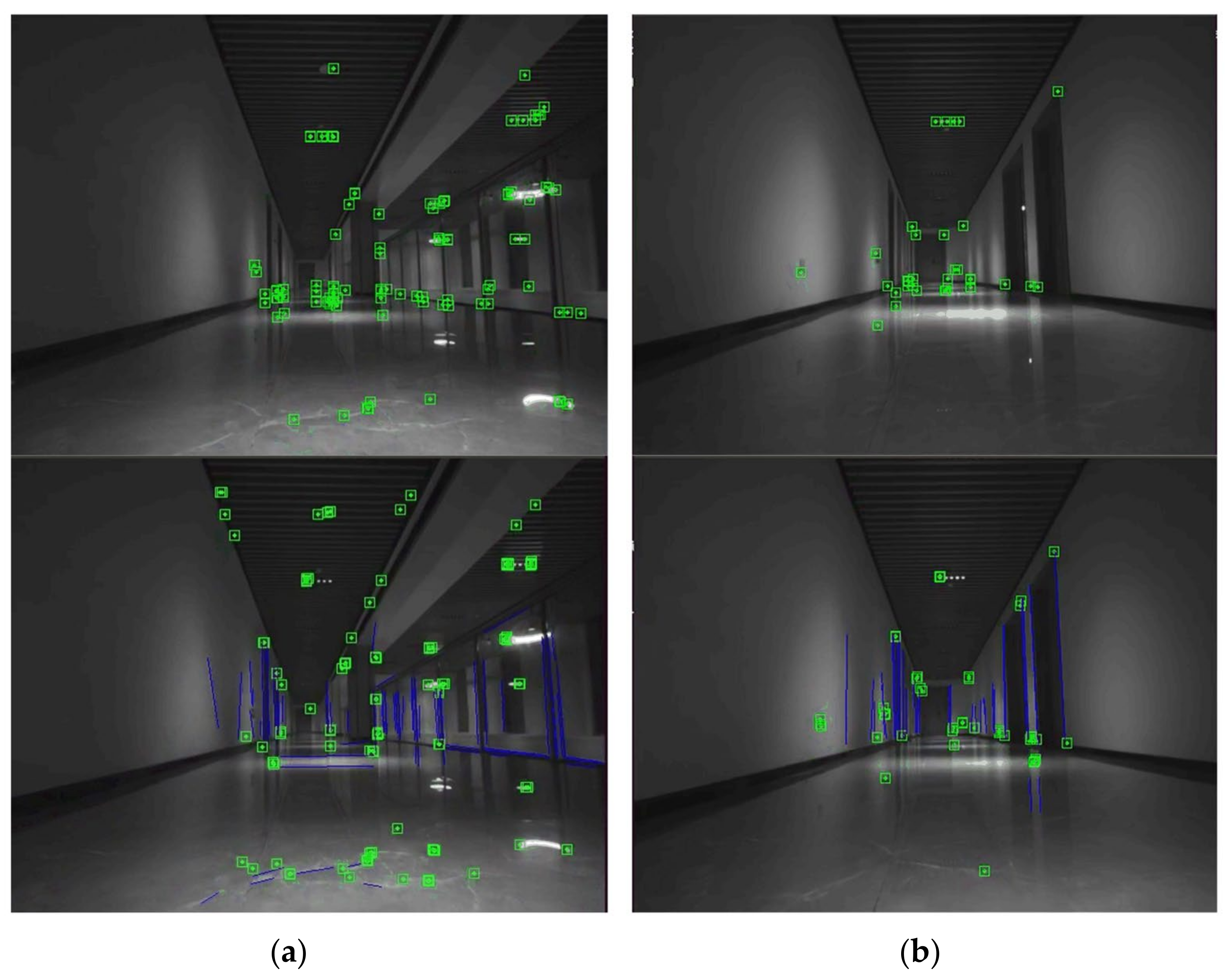
4.1.2. Line Features Detection
For the processing of line features, LSD is a widely popular method. However, its high computational cost usually prevents the system from running in real-time. In addition, LSD usually detects a large number of short line features that are difficult to match and are likely to disappear in the next frame, which not only wastes computational resources but also generates outliers for which matching line features cannot be found. To improve the real-time performance of the line feature extraction, we use EDlinesalgorithm to detect line features instead of LSD. EDlines utilizes an edge-drawing algorithm to generate edge pixel chains that have a faster running speed, about 10 times faster than LSD for a given equivalent image, while maintaining essentially the same accuracy [
1]. Therefore, using the EDlines algorithm is more suitable for visual SLAM than LSD.
However, it is worth noting that EDlines is more likely to detect curves [
24], which may degrade the performance of the system and affect the accuracy of the SLAM system. EDlines calculates parameters such as the length and direction of a line segment, but not the curvature of the line segment. Therefore, we introduce the curvature estimation method. After the line segment detection, the curvature is calculated for each line segment to determine the curvature degree of the line segment. This is done by traversing the pixel points of the line segment, and then calculating the curvature of each point. Finally, we average the curvature of all points to get the average curvature of the line segment. After that, we make a threshold judgment based on the curvature value of the line segment and filter out the line segments with the required curvature. Based on the experiment, we choose a maximum curvature threshold of 0.02, after which we discard the line segments that exceed the threshold because they increase the chances of false matches later on.
In addition, although EDlines can run without tuning parameters, when line features are applied in SLAM, we need more long line segments that can be tracked stably. Short line segments may be obscured in the next frame, making matching difficult, and the processing of a large number of useless short segments increases the computation time. Therefore, we add a filtering criterion to the original EDlines method of selecting the minimum line segment length based on different pixels, i.e., determining the length based on the number of feature points. The core idea is that, when the number of feature points is larger than the threshold
, our goal is to filter out the long line segments with higher quality to further improve the accuracy of matching. When the number of feature points is less than the threshold, we need to detect as many line segments as possible to improve the overall tracking robustness of the system. The minimum line segment length is calculated as follows.
where
is the ratio parameter for the minimum line segment length, which is formulated as Equation (2), and the rest of the parameters are the same as defined in EDlines, where
is the pixel side length of the image, and
is the probability of the binomial distribution calculation, which is used to indicate the line direction accuracy and usually takes the value of 0.125.
where
stands for the number of extracted feature points for the
i-th frame, and
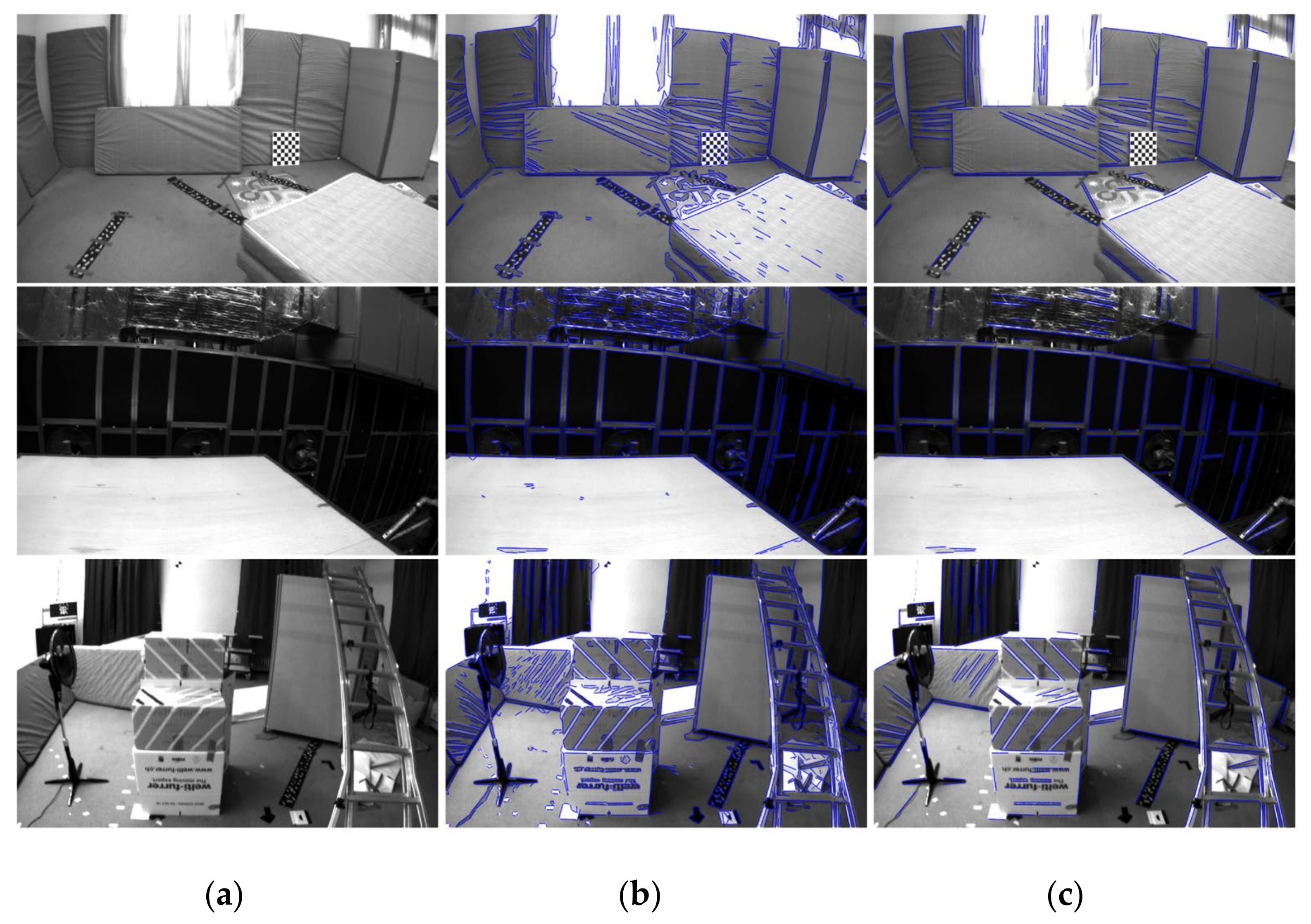
equals 20. The final result of the improved line segment detection is shown in
Figure 2.
4.1.3. Line Matching
For stereo matching, as with most methods, we selected the 256 bits LBD [
21], which contains geometric properties and appearance descriptions of the corresponding line features, and then the KNN method of Hamming distance is used to match along with the corresponding relation between the lines. To reduce outliers, we also refer to the PL-SLAM [
11], to allow for possible occlusions and perspective variations in real-world environments, where line pairs are not considered to be matched if their lengths differ by more than twice. In addition, if the distance between the midpoints of two lines on the image is greater than a given threshold, the line pairs are considered as mismatched. Finally, we use the useful geometric information provided by the line segments to filter out line matches with different orientations and lengths, as well as those with large differences in endpoints.
4.2. Motion Estimation
The tracking part consists of two main phases. The first stage of initial pose estimation includes three tracking methods: tracking with reference keyframes, tracking with constant velocity models, and tracking with reposition, which aim to ensure that the motion can be followed in time, but the estimated pose is not very accurate. After that, the pose will be optimized in the part Track Local Map.
4.2.1. Initial Pose Estimation Feature
When the map initialization is complete, if the current velocity is null and IMU has not completed the initialization, the initial pose estimation is performed in tracking in reference keyframes mode. Firstly, the point and line features between the current frame and the reference frame are matched, and then the pose of the last reference keyframe is used as the initial value of the pose of the current frame. After that, the pose will be optimized in the part Track Local Map. In addition, we use a more stringent condition to determine whether the tracking is successful, unlike ORB-SLAM3. Tracking is only successful if the number of matched interior points plus the number of line segments exceeds 15, even in the case of IMU.
If the IMU initialization is complete and the state is normal, we use the constant velocity motion model for initialized pose estimation and directly use IMU to predict the pose, otherwise, the difference of pose is used as the velocity. If the sum of matching pairs of points and lines is less than 20, we will expand the search radius and search again. After that, if the number is still less than 20 but the IMU status is normal at the moment, we add this status as pending. After the pose is optimized and the outer points are removed, tracking will be considered successful if the remaining matching quantity is still greater than 10.
If both of the above modes fail, the relocalization mode is used. First, we detect the candidate frames that satisfy the relocation conditions, and then search for the matching points and lines between the current frame and the candidate frames. and use EPnP for pose estimation if the pair of point and line matches is greater than 15. Finally, the pose will be optimized in the part Track Local Map.
Afterwards, we optimize the poses again with local map tracking according to the state of IMU, as specified in
Section 5.
4.2.2. Adapting Weight Factor Based on Experiment
Compared to point features, the endpoints of line segments are not stable and may be obscured when moving from the current frame to the next frame, resulting in larger line projection errors than for points. Therefore, we balance the reprojection error of the line according to the number of matched interior points, which can reduce the positional estimation error. When the number of interior point matches is small, we will increase the reprojection error weight
W of the line features and, conversely, if there are enough interior point matching pairs, we will decrease the reprojection error weight. In addition, the length of a line segment is also related to the size of the error. Generally speaking, a longer line segment is more robust and less likely to be lost by tracking. Therefore, based on the strategy in ORB-LINE-SLAM, we improve the reprojection error adapting factor
of line features which is formulated as:
where
stands for the groups of the sets of point matches,
stands for the total number of elements of group
,
is an operator which gives the integer part of a division,
stands for the length of segment
, and
stands for the average length of all line segments of the current frame. When the number of points increases, the weight
will decrease, because the line features are unstable compared to the point features, and the whole system will be more inclined to the point-based SLAM system if there are enough points, but more inclined to the line-based SLAM system when there are not enough points. In addition, a reasonable threshold
provides a good prior situation for the next tracking, while for the weight
we hope to find the best balance between the projection errors of the points and lines. Since the reprojection error of point features is more reliable than that of line features, we need to adjust these two parameters. The values of threshold
and weight parameters
will be described in detail in Experiment A.
4.3. KeyFrame Decision
As for the selection of keyframe, we need to ensure that it does not cause redundancy, but also ensure the validity. The keyframe selection strategy of ORB-SALM3 is worth learning. The selection of keyframe is initially based on loose standards, with subsequent elimination based on redundancy in the co-visibility graph. Therefore, our system follows the keyframe selection strategy of ORB-SLAM3 while adding a new judgment condition of keyframes for line features:
- (1)
If the number of line features tracked in the current frame is less than one-quarter of the number in the last reference keyframe, we insert the keyframe;
- (2)
Current frame tracked at least 50 points and 25 lines.
After that, the current frame is constructed as a keyframe, and the keyframe is set as a reference keyframe for the current frame, and a new map point is generated for the current frame.
6. Loop Closing
Current visual inertial SLAM systems basically follow the approach in ORB-SLAM2 for loop detection, which is based on the bag-of-word with point features only. However, the low texture or frequent illumination variations lead to wrong detection of the traditional point feature-based BoW. Therefore, we use a loop closing method based on the combination of point and line features to add line features to the loop detection. Meanwhile, we propose a combined time and space based adjudication method to weight the similarity score of the point and line features, to more fully take advantage of the data correlation from the line features, and to reduce the error detection, in order to improve the robustness of the system in low-texture and low-light situations.
Since the LBD descriptors of the line features and the rBREF descriptors of the ORB features are both binary vectors, we can use clustering of the two descriptors to build the point and line K-D tree to create a visual dictionary that combines the point and line features. After that, we propose a combined weighted point-line similarity score criterion with an adaptive weight. From the perspective of space, for the similarity of the single features, we consider weighting by the proportion of the features to the sum of all the features. In addition, since it is difficult to describe the image as a whole well with features that are too clustered, it is also necessary to weight the point and line features based on the dispersion of the distribution of point and line features in the image. The distribution of point features is calculated as standard deviation
based on their coordinates
, and the distribution of line features is calculated as standard
deviation based on the midpoint coordinates.
where
and
are the groups of point features and line features in the image, respectively, and
and
are the number of points and lines extracted in the image, respectively. The coordinates of the points in the candidate keyframe are
and the coordinates of the midpoint of the lines in the candidate keyframe are
.
For the combined similarity weights of points and lines, traditional methods such as PL-SLAM and PEI-SLAM only set the similarity weights of both points and lines to 0.5, but with low texture features, the number of points will be reduced and the number of lines will be increased, which will tend to weight the similarity scores of the lines more. Therefore, we set the weight
on the similarity of the lines based on the final value of the gradient threshold
at the point feature extraction of that frame, defined as:
Finally, the total combined point-line similarity score is defined as follows:
where,
and
are the similarity scores of points and lines relative to the candidate keyframes, respectively. The single feature similarity score for frame
is calculated as follows:
where,
and
are the corresponding BOW vectors of frame
and candidate keyframe, respectively.
Finally, we decide whether a loop closing has occurred by comparing the total score with the threshold value. In addition, from the perspective of time, since neighboring keyframes tend to have more of the same features, the loop closing can only be considered effective when two frames are more than 10 frames distant from each other in order to avoid misclassification.
7. Experimental Results
In this section, we experiment on the adapting weight factor to select the best parameters. In addition, we evaluate the performance of PLI-SLAM in comparison to popular methods on EuRoC MAV [
15], including the visual-inertial SLAM system based on point features (ORB-SLAM3), the pure visual SLAM system based on point and line features (ORB-LINE-SLAM), and the visual-inertial SLAM system based on point and line features (PEI-VINS). We also present the performance of our system using the original EDlines to verify the effectiveness of adding curvature detection and suppression of short lines to the EDlines. For PEI-VINS, we present the results provided in the paper directly, as it does not have the full code. For all other algorithms, we used the original authors’ parameters tuned for the EuRoC dataset. Meanwhile, the initial parameters of PLI-SLAM are the same as those set by ORB-SLAM3. The metric for the evaluation we used is absolute trajectory error (ATE) [
31]. Due to the fact that real-time performance is an important indicator of the SLAM process, we present the performance of the average processing time per frame on each sequence of the EuRoC dataset to verify the validity of our use of EDlines instead of LSD. Finally, the test in a real environment verifies the validity of our approach.
All experiments have been run on an Intel Core i7-8750 CPU, at 2.20 GHz, with 16 GB memory, using only CPU.
7.1. Adapting Weight Factor
The EuRoC MAV dataset provides three flight environments with different speeds, illumination, and textures, including two indoor rooms and an industrial scene. The first experimental sequence we selected is the V101 with slow motion, bright scene, and good texture. The second sequence we chose was the MH03 with fast motion, good texture, and bright scenes. The last sequence we selected, V203, is a motion blur, low-texture scene. We determine the best parameters to balance the line reprojection error based on the performance in three different environments, and also select ATE as the evaluation criterion. Referring to the threshold 20, at which tracking is considered successful, tracking starts by increasing the weights and thresholds simultaneously until the system reaches optimal accuracy.
Table 1 shows the average of the results of the three sequence run and, taking into account the randomness of multithreading, each sequence was run 30 times. From the results, for a fixed threshold, as the weighting factor increase, the absolute trajectory error roughly tends to first reach a minimum and then increase until no value of the weight parameter is likely to improve the results. The system achieves the best performance in different environments when
equals 60 and
equals 2.
7.2. EuRoC MAV Dataset Quantitative Evaluation on EuRoC MAV Dataset
Table 2 shows the performance of the above algorithms on all 11 sequences of the EuRoC dataset. The lowest absolute translation errors for each test are marked in bold. From the obtained results, our proposed PLI-SLAM significantly improves the robustness and accuracy to EuRoc, especially for the MH01 sequence with rich line features and challenging sequences, like MH05 and V203.
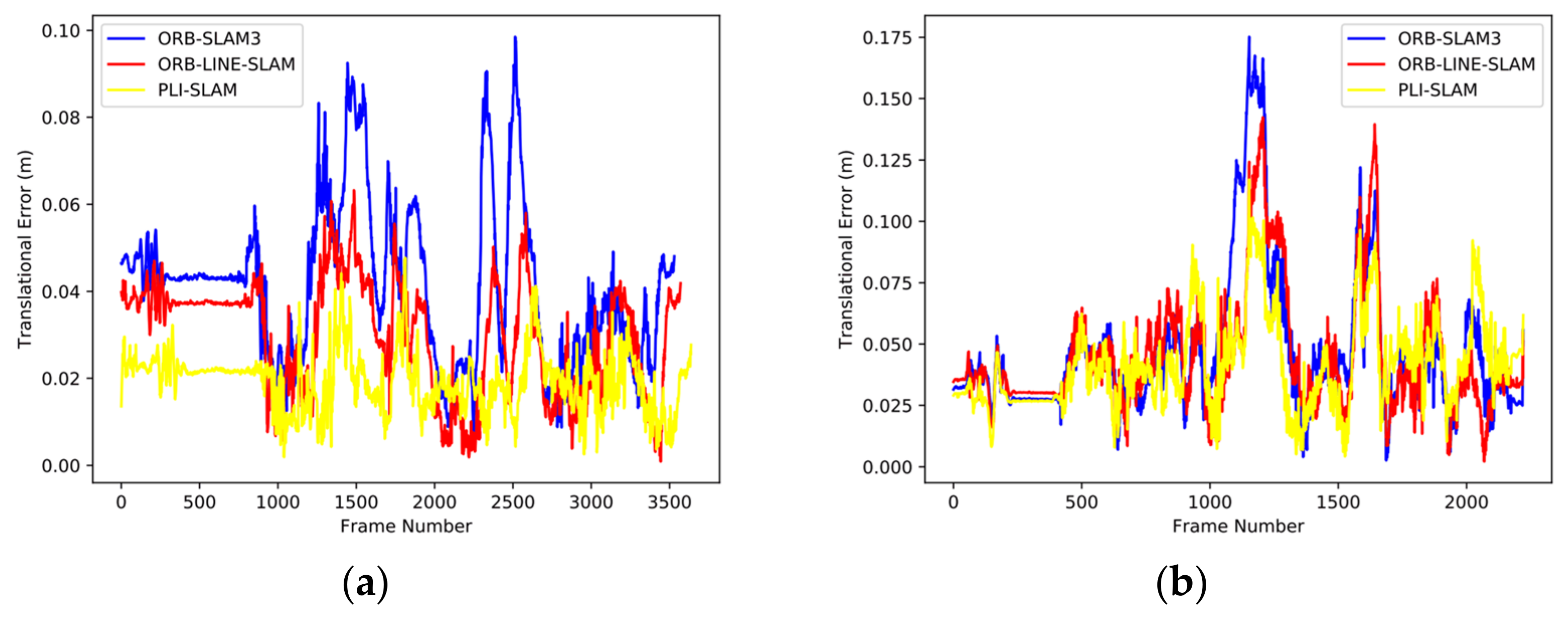
Figure 5 shows the details of the per-frame translation error for the MH01 and MH05, and the results show that our algorithm has the lowest trajectory error.
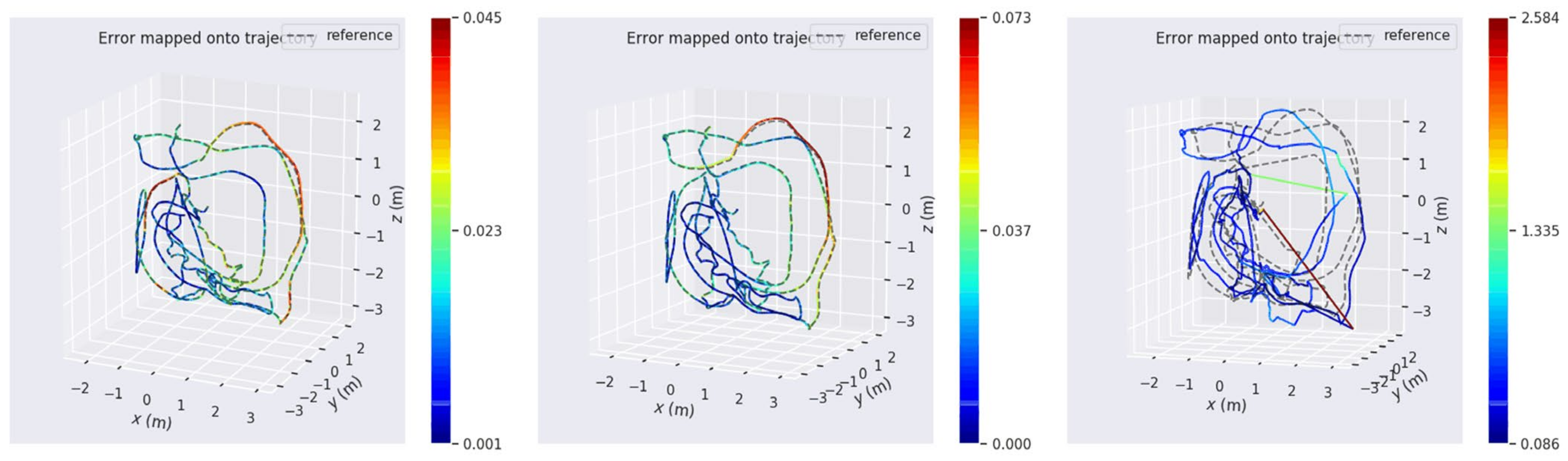
Figure 6 and
Figure 7 show the trajectory estimated and relative translation errors on the V203 sequence, which is a most challenging sequence. On this sequence, the purely visual SLAM system ORB-LINE-SLAM performed poorly, with multiple and severe deviations or lost tracking. The pose estimation was severely affected by severe motion blur, resulting in ORB-LINE-SLAM matching only few points and lines in some of these frames. In contrast, several other visual-inertial SLAM systems can operate robustly due to the combination of IMU, which allows the system to determine its own motion attitude through the angular velocity and acceleration information provided by IMU measurement, even in the state of pure vision failure.
At the same time, compared with the point feature-based visual inertia method, the use of high-quality line features can effectively improve the accuracy of the track. Especially, the medium-size factory scene in MH01 and MH03 sequences have a large number of well-structured line segment features, which is conducive to our system improving the trajectory accuracy of motion by using high-quality line features. However, using the original EDlines did not improve the system performance significantly, and even reduced the trajectory accuracy in a few sequences. This is also reasonable, because the reprojection error of line segments is less reliable compared to point features, and using low quality line segments will undoubtedly affect the system performance, which further proves the superiority of our solution. On the whole, it is discernible that PLI-SLAM significantly prevails among the 11 sequences.
In addition, we compare the performance using the bag of words based on point features only with that using the combined bag of words based on point and line features. From the results, the addition of line features in loop detection can significantly reduce the trajectory error. The main reason for this is, when calculating the similarity score, the point features reflect the local information of the image, which is not robust enough for the similar scene, and thus it is more likely to have an error loop. However, line features have higher dimensionality, larger coverage, and are more reflective of global information than point features. Meanwhile, the proposed adaptive weight similarity score criterion makes line features more reliable for loop closing in environments with rich line textures, and reduces false loop and trajectory errors compared to point features.
7.3. Processing Time
With regard to performance of time, we evaluated the average processing time per frame of different methods on each sequence, and the results are shown in
Table 3. From the results, the addition of line features increases the processing time of the system, especially in the detection of line features in tracking thread and loop closing thread, but still has advantages compared to LSD. Our system has 28% less average processing time per frame than ORB-LINE-SLAM even with the addition of IMU. This benefits from the speed advantage of EDlines in detecting line features in the tracking thread. In addition, IMU allows for less drift of the poses compared to a pure vision system, thus making a closed-loop correction or map fusion with smaller computational overhead. There is also an advantage in the running time of our system compared to the original EDlines, due to the filtering of the curves and shorts, which saves a lot of time in the subsequent computation of the line descriptors and matching. In addition, we also provide performance of PLI-SLAM with bag-of-words based on point features only, which is comparable to ORB-SLAM3 or even faster. This is due to the reason that we use gradient thresholding to extract point features, which avoids redundant features and reduces computing time in environments with rich point feature textures. However, PLI-SLAM with full bag of words will have a disadvantage in speed compared to ORB-SLAM3, even though it has a large improvement in accuracy. Therefore, we provide a bag of words in loop detection with autonomously selectable line features to achieve a balance in accuracy and speed.
7.4. Real-World Experiment
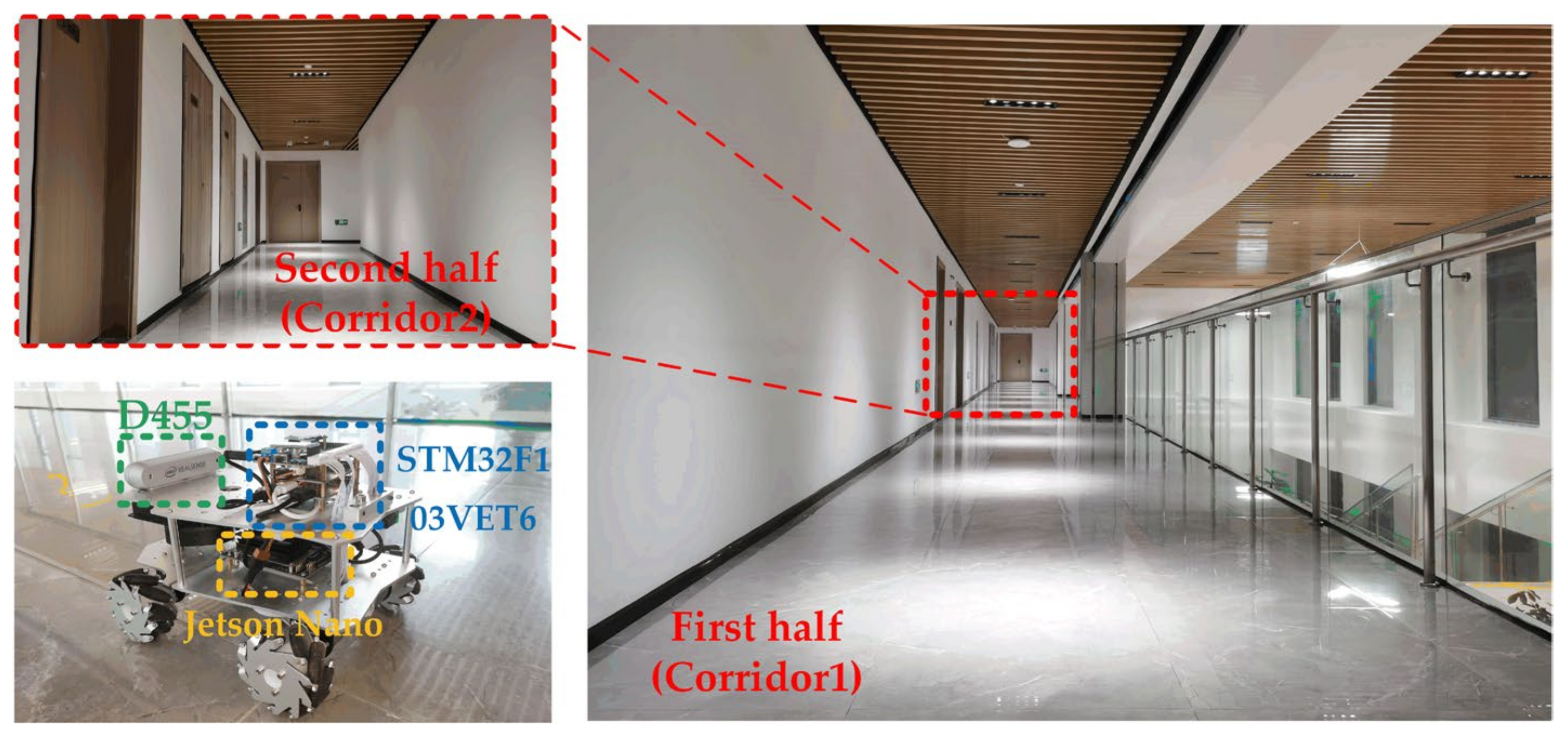
In order to verify the performance of the proposed method in real-world scenarios with fewer textures, we conducted experiments in Building 3, Yangtze Delta Region Academy, Beijing Institute of Technology, Jiaxing, China. The real-time data was acquired by a RealSense D455 consisting of a stereo camera (30FPS, 640 × 480) and an IMU (100 HZ). The equipment was calibrated and performed well before the experiment.
The test environment is a common indoor corridor including two scenes with different textures as shown in
Figure 8, and the texture features are compared with two typical sequences of EuRoC dataset as shown in
Table 4. Corridor1 is an open corridor with more texture and the Corridor2 is a narrow corridor where it is difficult to extract point features, but with many line features. The core purpose of our experiment is to prove the robustness improvement of line features to the system in an environment where it is hard to extract point features. The experimental platform is a four-wheeled Mecanum wheel robot, equipped with a ROS master (Jetson Nano) and a microcontroller (STM32F103VET6), which can set up the program of the microcontroller to obtain the true value of the length of the ground truth with a systematic odometry error of less than 0.5% by giving the target straight-line distance and speed. The target was defined as a line distance of 35 m, and the speed was set at between 0.2 m/s and 0.5 m/s. The robot moved from a rest, in the simplest form of linear motion. The topics of stereo and IMU released by the D455 camera will be collected in real time by recording a rosbag. Afterwards, the recorded rosbag will be played without any other processing to run algorithms. We quantitatively evaluate the ability to estimate the true scale by relative error
over the total length of the trajectory between the results and the ground truth [
32]. Finally, we visualize trajectories by the EVO evaluation tool and qualitatively compare the ability to work properly from the starting point to the end point.
The
of the two algorithms are shown in
Table 5. The results show that PLI-SLAM has a better ability to estimate the true scale in Real environment with low textures compared to ORB-SLAM3. As shown in
Figure 9, from the trajectory results of the two algorithms, PLI-SLAM has good robustness to low texture, while ORB-SLAM3 leads to a large error of visual-IMU alignment because of few point features extracted, which in turn leads to tracking fails.
Figure 10 further shows the performance of the both algorithms for the two corridors. In corridor 1, ORB-SLAM3 can extract enough point features to keep working properly, but please note that most of the point features extracted are focused on the right part of corridor 1, so that few point features can be extracted after entering corridor 2, and this finally fails. Conversely, PLI-SLAM can extract a large number of structural line features in both corridors and thus has good robustness. As a result, adding line features can greatly improve the robustness of SLAM in low texture environments.
8. Conclusions
In this paper, we proposed PLI-SLAM, a tightly coupled point-and-line visual-inertial SLAM system based on ORB-SLAM3, with faster and improved EDlines, instead of the widely used LSD. Our approach achieves good robustness and accuracy in low-texture environments by adding line features and adapting weighting factors for reprojection error. Besides, the multi-sensor information fusion of IMU and camera enables the PLI-SLAM system to operate robustly in scenarios where pure vision may fail. Compared to several different types of SLAM system, our method has great advantages in experiments with the EuRoC dataset, especially on the V203 sequence, which confirms the robustness and accuracy of our system. Meanwhile, PLI-SLAM also has time advantages over methods using LSD. Experiments in real environments also show the superiority of the proposed PLI-SLAM in low texture environments.
In the future, we will look for more ways to reduce the computation time of the line features or combine other structural features to make the system further improve in speed and accuracy.


