Article

Rapid Emergency Response Assessment of Earthquake-Induced Landslides Driven by Fusion of InSAR Deformation Data and Newmark Physical Models

School of Civil Engineering, Southwest Jiaotong University, Chengdu 610031, China
*
Author to whom correspondence should be addressed.
Remote Sens. 2023, 15(18), 4605; https://doi.org/10.3390/rs15184605
Submission received: 4 August 2023 / Revised: 27 August 2023 / Accepted: 8 September 2023 / Published: 19 September 2023
(This article belongs to the Section Remote Sensing and Geo-Spatial Science)

Abstract

:
Strong earthquakes induce a large number of secondary disasters, such as landslides, which bring serious challenges to post-disaster emergency rescue, and the rapid and accurate assessment of earthquake-induced landslide disasters is crucial for post-earthquake emergency rescue. This research aims to propose an emergency assessment model that is suitable for post-earthquake landslides, specifically targeting the first 72 h after an earthquake for emergency rescue guidance. The model combines remote sensing technology and the Newmark physical mechanics assessment model to form the InSAR Data–Newmark Physical Fusion Driver Model (IDNPM), which comprehensively considers the dynamic deformation of the ground surface and geological features. To validate the predictive performance of the IDNPM, the model is applied to the 5 September 2022 Luding earthquake event and the 8 August 2017 Jiuzhaigou earthquake event. The landslide qualitative evaluation, confusion matrix and Receiver Operating Characteristic (ROC) curve are utilized for quantitative assessment. The results show that the IDNPM can effectively reduce the false negative and false positive errors in landslide prediction by utilizing the SAR deformation information, and to a certain extent, it accounts for the dependence of the Newmark model on the accuracy of empirical formulas and geotechnical parameters. For the Luding earthquake event, the IDNPM shows an accuracy improvement of 10.296% compared to the traditional Newmark model. For the Jiuzhaigou earthquake event, there is also an improvement of 3.152%, with a promising generalization performance. The simplicity and ease of operation in constructing the model are accompanied by high reliability and accuracy. The research findings provide essential references for the development of post-earthquake landslide emergency prediction models and offer robust data support for emergency rescue and recovery efforts in earthquake-stricken areas in the future.

Graphical Abstract

1. Introduction

Major earthquakes often trigger a multitude of secondary disasters, such as large-scale landslides, instantly burying individuals and structures, causing extensive damage to critical infrastructure such as bridges and roads, and impeding prompt emergency responses and aid delivery [1,2]. These consequences result in significant losses of life and substantial economic repercussions. The inherent unpredictability of earthquakes [3] means that the exact timing and location of an earthquake’s occurrence cannot be accurately determined. Therefore, obtaining rapid and accurate assessment results of earthquake-induced landslides and the ensuing disaster in the immediate aftermath of an earthquake holds paramount importance for emergency responses, rescue operations and subsequent recovery and reconstruction efforts [4,5].
Currently, the primary means of assessing post-earthquake landslide hazards include traditional ground surveys, aerial remote sensing and unmanned aerial vehicle (UAV) aerial photography. Traditional ground surveys rely on investigators entering the disaster-stricken area for on-site investigations, which require a significant amount of time and human resources. However, in the event of road closures and communication disruptions caused by earthquakes, conducting immediate ground surveys poses enormous challenges. With the development and maturity of Geographic Information Systems (GIS) and remote sensing technology, earthquake landslide identification based on remote sensing images has become not only the core and foundation of landslide research but also the most effective method of obtaining extensive disaster information in affected areas [6,7,8]. However, this method is limited by adverse weather conditions, as remote sensing interpretation becomes difficult when faced with unfavorable weather conditions, making it challenging to rapidly acquire post-disaster information. UAVs can conduct aerial photography in the disaster area in a timely manner, capturing high-resolution images and videos. Based on the obtained data, the extent of damage, safety conditions and emergency needs in the affected area can be assessed, providing a scientific basis for rescue operations. However, UAVs have limited endurance and flight range, making it equally challenging to complete a comprehensive disaster assessment of the entire area in the immediate aftermath of an earthquake. Therefore, it is necessary to propose better technological means for emergency assessments of post-earthquake landslides.
Currently, the emergency assessment of post-earthquake landslides is still in the exploratory stage and has become a highly focused research topic [7,8,9]. In this regard, algorithmic models trained on historical data and limit-equilibrium-based mechanical models are the main prediction methods, both of which have shown promising practical applications. However, these two methods have certain limitations. For instance, algorithmic models lack a deep understanding of the mechanisms behind landslide occurrences and may not adequately consider the inherent characteristics of natural slopes. On the other hand, mechanical models rely on the accuracy of empirical formulas and geotechnical parameters, leading to lower precision in practical applications. In summary, post-earthquake situations often face challenges such as disrupted transportation hindering traditional ground surveys, limitations in satellite remote sensing applications due to cloud cover and difficulties for UAVs to rapidly obtain timely assessment results immediately after the earthquake [9]. Therefore, it is necessary to continue developing new emergency assessment models for post-earthquake landslides to overcome the limitations of existing methods.
Interferometric Synthetic Aperture Radar (InSAR) technology has been widely applied in various fields, such as ground subsidence [10,11], the early identification of landslides [12,13] and post-earthquake landslide interpretation [14,15,16], due to its all-weather capability, high precision, high spatiotemporal resolution and robust interference resistance. Among these applications, Small Baseline Subsets-Interferometric Synthetic Aperture Radar (SBAS-InSAR) significantly reduces spatial decorrelation between data points and effectively mitigates the influence of terrain residuals and atmospheric noise. It has received recognition from many scholars for early landslide identification and deformation monitoring. Although SBAS-InSAR technology is constrained by weather conditions in the immediate aftermath of an earthquake, the analysis of historical remote sensing images prior to the earthquake enables effective identification of unstable slopes. We observed that unstable slopes are often subjected to both direct seismic impacts and secondary effects induced by earthquakes, resulting in a further reduction in their already weak stability [17]. Seismic forces make these unstable slopes more susceptible to instability, leading to secondary disasters, such as landslides. However, it is not feasible to directly determine the extent of post-earthquake landslide disasters based solely on the identification of unstable slopes prior to the earthquake. Several issues need to be addressed: (a) The InSAR identification of unstable slopes only provides pre-earthquake information and cannot evaluate the post-seismic stability behavior of originally stable slopes. (b) InSAR technology overlooks the inherent characteristics of natural slopes, and the identification of anomalous areas based on deformation rates cannot accurately determine whether a landslide will be triggered under seismic forces. In light of these challenges, the integration of limit-equilibrium-based mechanical models can effectively address these issues.
The Newmark model, based on mechanical principles, is widely used for the quantitative analysis of slope instability. This method enables the rapid prediction of earthquake-induced landslides in the study area based on seismic parameters and data related to natural slopes [18,19]. By combining the Newmark model with InSAR technology, the shortcomings of InSAR technology in terms of landslide mechanisms can be addressed. Furthermore, SBAS-InSAR technology can process long-term sequences of SAR data, providing information on large-scale ground deformation and changes in unstable slopes. This partly compensates for the Newmark model’s reliance on empirical formulas and geotechnical parameters’ accuracy. Taking into account regional geological conditions and landslide types, as well as recognizing the importance of vulnerability assessment results and surface deformation information, a weighted overlay approach can be employed to integrate the seismic assessment results from the Newmark model and the surface deformation information from InSAR technology into a geographic information system environment. Through this integration, a post-earthquake emergency assessment model can be obtained that is characterized by rapid responsiveness and stable reliability.
This study aims to propose a novel emergency assessment model tailored to post-earthquake landslides, specifically catering to the critical 72 h period following a seismic event for emergency rescue demands. The InSAR Data–Newmark Physical Fusion Driver Model (IDNPM) is constructed by integrating pre-earthquake InSAR deformation data with post-earthquake Newmark physical model evaluation results to facilitate the rapid assessment of seismic-induced landslides. To verify the feasibility and performance of the IDNPM, the model is applied to the 5 September 2022 Luding earthquake event in Sichuan Province as the primary research basis for post-earthquake rapid landslide evaluation. A comparison and validation of the IDNPM’s results are conducted against the actual distribution of earthquake-induced landslides. Through this research, the goal is to achieve the timely identification of the distribution and scale of post-earthquake landslides within a few hours after the seismic event, providing data support for emergency rescue and response operations. The findings of this study contribute new technical means for rapid emergency assessments in earthquake-stricken areas, holding significant implications for disaster prevention, mitigation and post-disaster emergency management in China.

2. Research Techniques and Methods

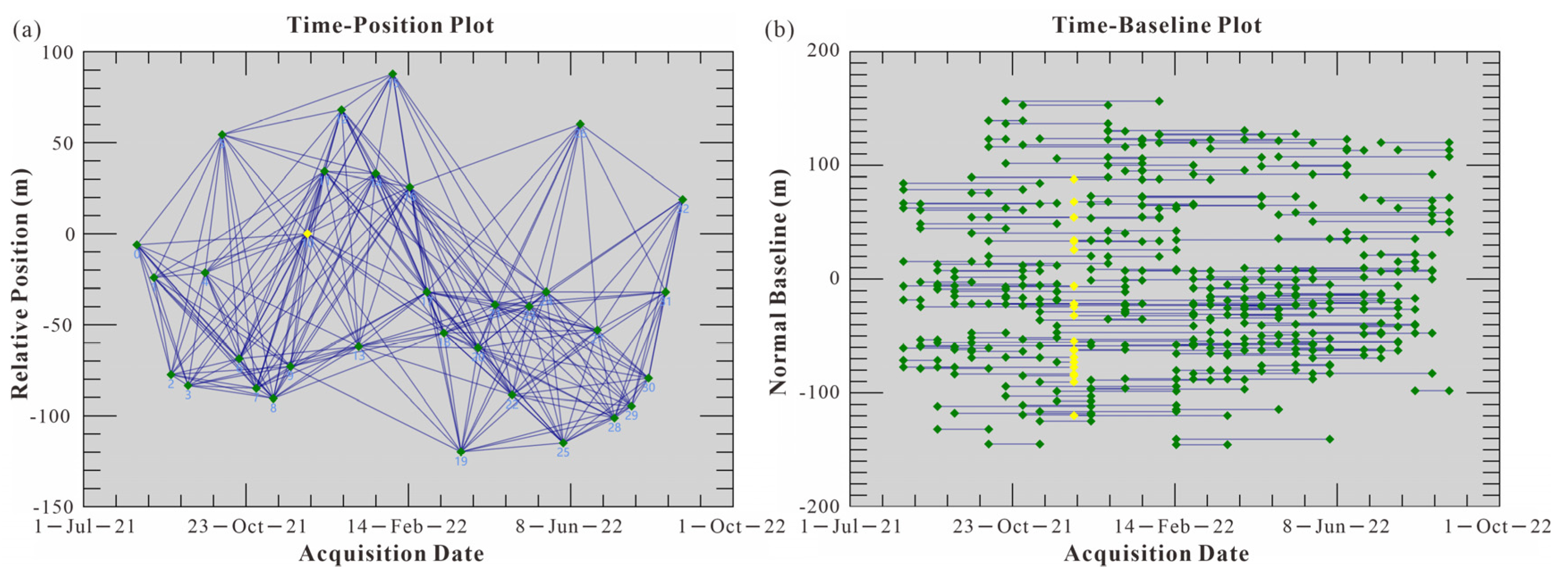
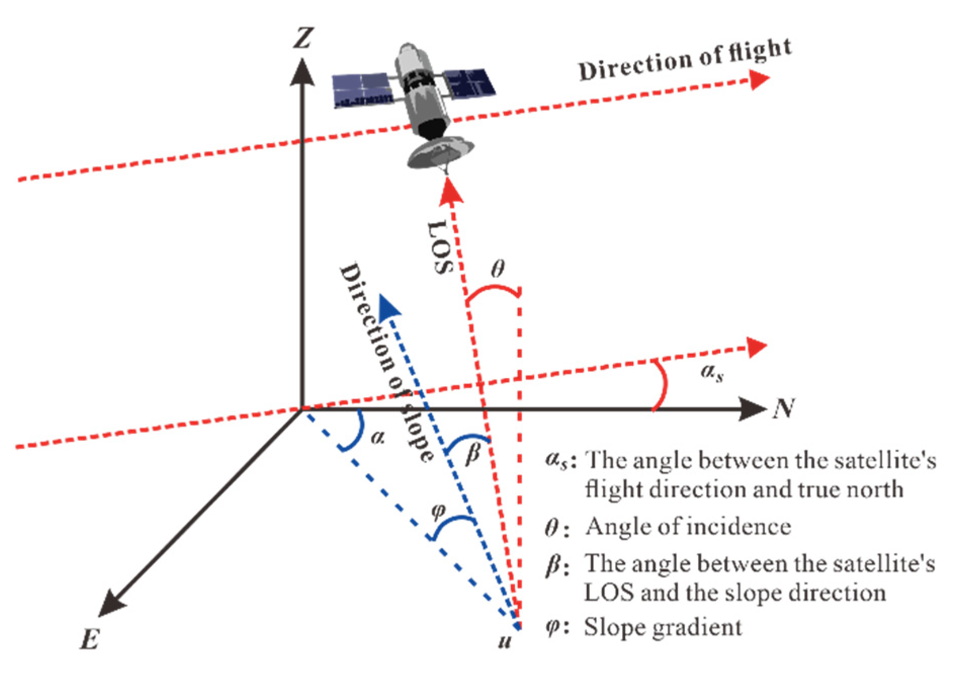
2.1. SBAS-InSAR Technology

The SBAS technique was designed in 2002 [20], and the basic principle of the method is to generate coherent interferograms with short time–space baseline image pairs and then to deconvolve the interferometric phase. The effect of spatio-temporal denoising can be better overcome to extract as much practical information about the distributed scatterers as possible. The N + 1 SAR image of the same region is acquired at a fixed time to produce M differential interferograms and satisfies Equation (1). For the j ( j = 1, 2, …,) differential interferogram generated by two images at the moments of t A and t B ( t A < t B ), the interferometric phase at any point is calculated with Equation (2).
N + 1 2 M N ( N + 1 ) 2
δ φ j = φ t B φ t A 4 π λ ( d t B d t A ) + Δ φ j t o p o + Δ φ j a t m + Δ φ j n o i s e
where δ φ is the interference phase at any point; φ t is the phase corresponding to any time; d t is the cumulative shape variable corresponding to any time; t is the time; λ is the wavelength; Δ φ j t o p o is the atmospheric delay phase; Δ φ j a t m is the residual topographic phase; and Δ φ j n o i s e is the noise phase.

2.2. Newmark Physical Mechanics Model

Based on the Newmark cumulative displacement model constructed by the limit equilibrium theory [21], the model treats the sliding part of the landslide as a rigid body on the slope where motion occurs, and the minimum acceleration required to be applied on the object is called the critical acceleration ( a c ). The slope reaches the limit equilibrium state when the intensity of local vibrations reaches the ability of the landslide body to resist earthquakes. When the intensity of local vibrations continues to increase, the slope body slides, i.e., a landslide disaster occurs. After obtaining a c , the permanent displacement value ( D n ) is calculated by integrating twice the seismic acceleration timescale that exceeds the critical acceleration.
a c = ( F s 1 ) g sin α
F s = c γ h sin α + tan φ tan α m γ w tan φ γ tan α
D n = t t [ a ( t ) a c ]   d t   d t
where a c is the critical acceleration; g is the acceleration caused by the Earth’s gravity; α is the angle at which the center of mass of the potential landslide mass starts to move from the horizontal direction, which can be generally approximated as the slope angle; F s is the static safety factor; c is the effective cohesion of the geotechnical body (kPa); γ is the geotechnical body weight (kN/m3); h is the thickness of the potential landslide body (m); φ is the effective internal friction angle of the geotechnical body (°); m is the proportion of the saturated part of the potential landslide body to the total thickness of the landslide body; γ w is the groundwater heaviness; and a ( t ) is the acceleration time range function, which is obtained from the seismic observation of the seismic station.

2.3. InSAR Data–Newmark Physical Fusion Driver Model

Some scholars have integrated InSAR technology with landslide susceptibility evaluation results, all of which use InSAR deformation as a covariate or as a dynamic verification means to complete landslide susceptibility evaluations [22,23,24,25], and they have achieved good application results. However, the above methods rely on the availability of landslide remote sensing interpretation conditions after the earthquake as well as mastery of a complete landslide inventory, which obviously does not meet the requirements of the first-time landslide disaster emergency assessment after the earthquake. Therefore, the IDNPM proposed in this paper has significance in the emergency assessment of the critical time for post-earthquake rescue. The contingency matrix and the weighted overlay method are two commonly used integration methods, of which the weighted overlay method is easier to operate. In order to facilitate a rapid response after an earthquake, the model adopts the weighted overlay method, as shown in Equation (6).
I N = a × I n S A R + ( 1 a ) × N e w m a r k
where I N indicates the calculated IDNPM calculation results and a is the empirical weight value.
Determining the empirical weight values requires an extensive literature survey and an analysis of examples and prioritization between two factors, i.e., relative importance. Examples and experiments [17] have proven that slopes with pre-earthquake damages and deformations are more likely to be destabilized under seismic action, and pre-earthquake surface deformation is roughly proportional to the probability of destabilization. The Newmark method is an effective method for calculating the displacement of earthquake slopes, and its calculated displacement values directly characterize the probability of natural slope instability after an earthquake. The results of the InSAR deformation and the Newmark physical model have a direct influence on the final results of the IDNPM. Referring to the results of previous studies [22,23], and considering the limitations of the InSAR method and the importance of geological conditions on landslide development [26], an empirical weight value of 0.39 was taken in this study and combined with Equation (6) to form the final post-earthquake rapid emergency response assessment results of landslides. Figure 1 shows the flow chart of this model’s construction.

3. Study Area and Data Preparation
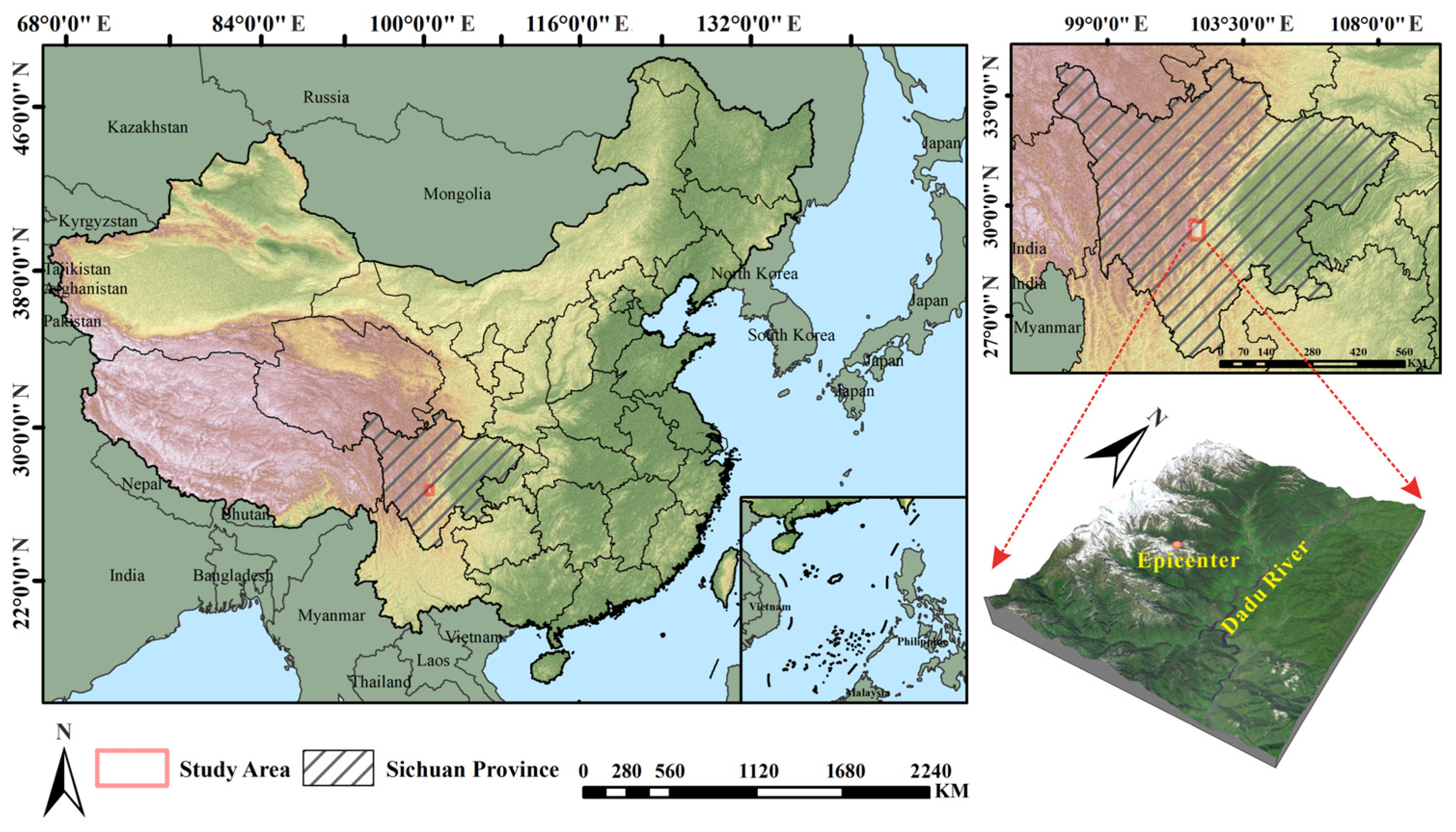
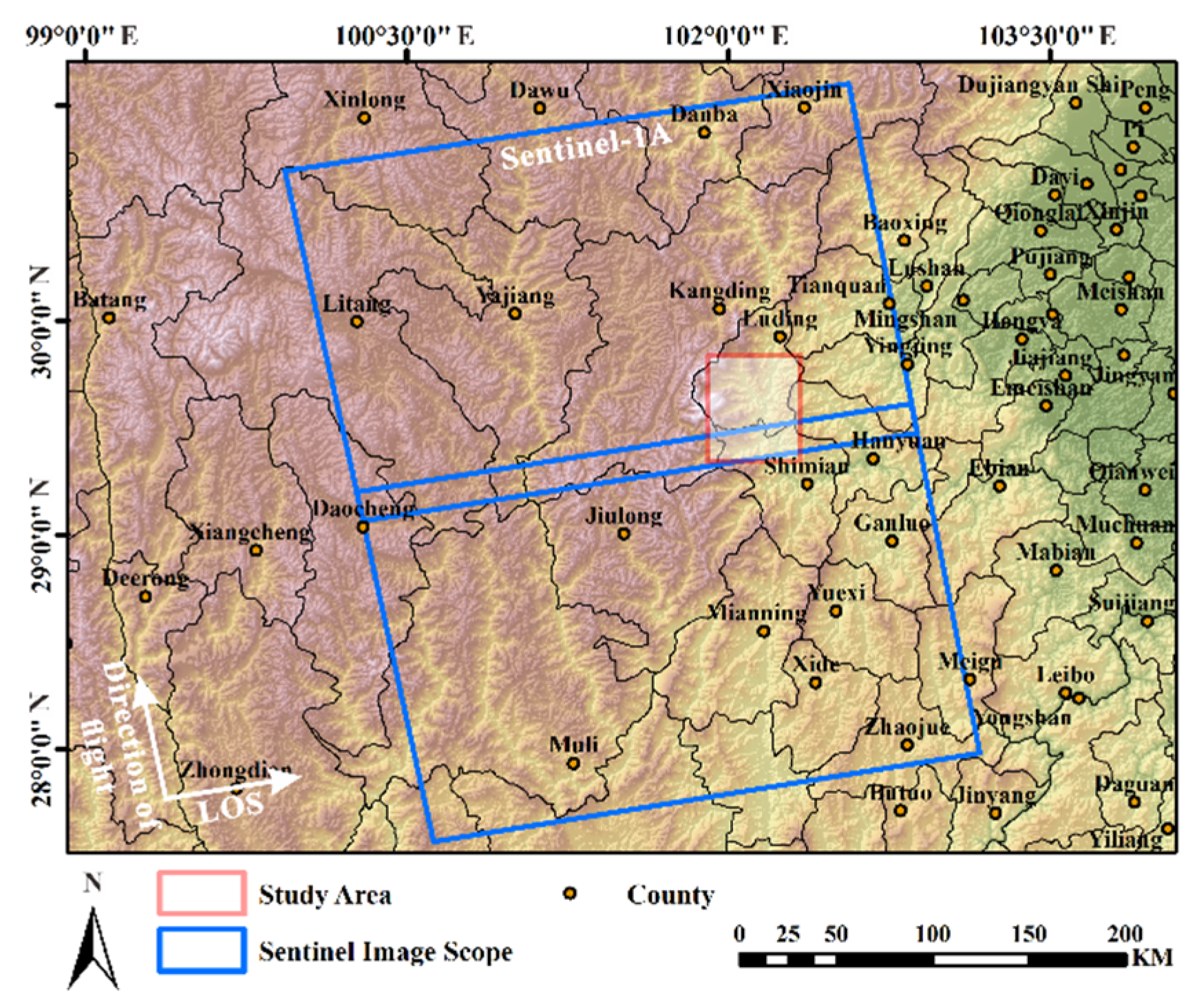
3.1. Study Area

The Ms 6.8 earthquake occurred on 5 September 2022 in Luding County, Ganzi Prefecture, Sichuan Province, at a source depth of 16 km, with the epicenter located in the town of Moxi, Luding County, at the geographic coordinates of (29.59°N, 102.08°E) (see Figure 2). The seismogenic fault is the Xianshui River Rift on the southeastern edge of the Tibetan Plateau, and the source mechanism is a strike-slip type [27]. The earthquake induced a large number of geological hazards, causing collapsed houses, roads and bridges, as well as casualties [8]. As of 14 September, relevant data reflect that this earthquake caused 97 deaths, 423 injuries and 30,317 emergency relocations and caused economic losses that are estimated to exceed 20 billion yuan [28].
After the earthquake, ground mapping could not be carried out immediately due to transportation routes being blocked. Moreover, the first clear high-resolution remote sensing images could not be obtained until the fifth day after the earthquake due to weather conditions [8]. During the 72 h critical rescue time after the earthquake, UAV technology also faced a dilemma in which it was difficult to obtain large-scale disaster data after the earthquake. Therefore, it is very necessary to carry out post-earthquake landslide rapid emergency assessments to provide timely support for post-earthquake emergency rescues [8,29].

3.2. Data Preparation

The SBAS-InSAR technique was used to analyze the pre-earthquake deformation in the study area. This was performed with 33 scenes (12 d time monitoring interval) of Sentinel-1A ascending orbit single-view complex (SLC) images from 7 August 2021 to 26 August 2022 using ENVI 5.3 and SARscape 5.2.1 software, with the data coverage shown in Figure 3. The images were in the interferometric wide swath (IW) and VV polarization mode, with an incidence angle of 34.284°, a flight azimuth of 347.339° and a spatial resolution of 5 × 20 m. Moreover, the orbital accuracy was improved by using the precision AUX_POEORB orbital data file provided by ESA, and a 1 arc second image with a resolution of 30 m was used. The Digital Elevation Model (DEM) of the 1 arcsecond product with a resolution of 30 m was used as a terrain reference.
In addition, pre-earthquake topographic data, engineering geological rock set information and the first post-earthquake release of ground shaking intensity data were obtained, in which the 1:500,000 scale regional geological information was selected for the engineering geological rock set. These data were used for the rapid assessment of earthquake-induced landslides in the Newmark model, and the specific data and sources involved are shown in Table 1.

4. Results and Analysis

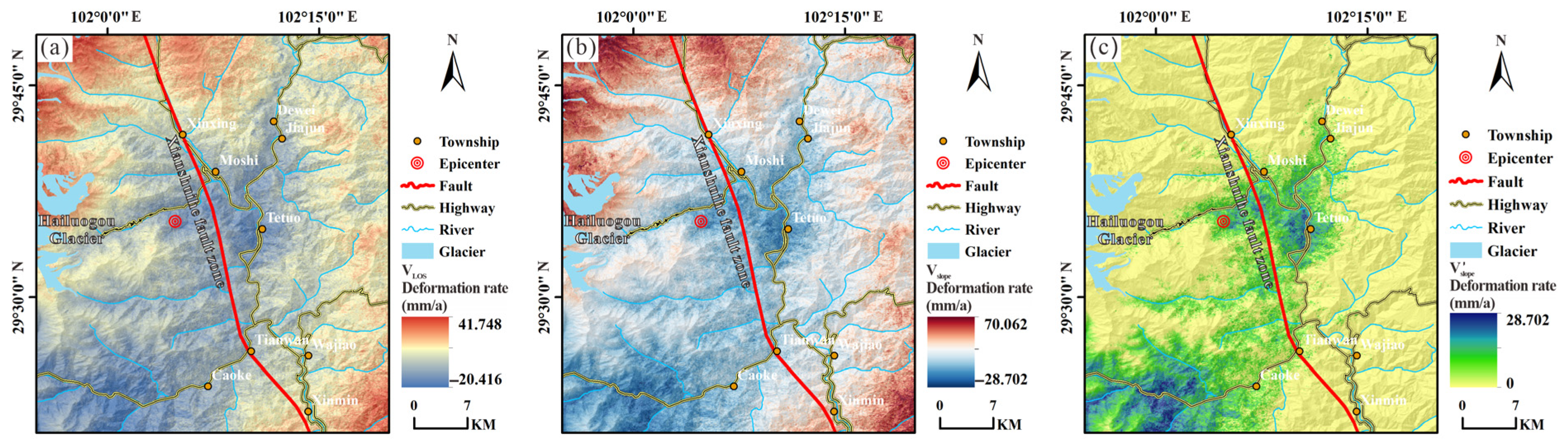
4.1. Results of Surface Deformation Based on SBAS-InSAR

4.1.1. SBAS-InSAR Deformation Rate Acquisition

SAR imagery from the year prior to the earthquake was selected as the study data, and the temporal baseline threshold was set to 120 days. The spatial baseline threshold was set to 2%, resulting in a total of 248 interferometric pairs (see Figure 4). The yellow dots represent the imaging time of the reference master image, and the green dots represent the imaging time of the remaining 32 view images.
The synthesized interferograms are inverted twice and geocoded to generate the deformation data along the radar line of sight (LOS) direction of the ground surface. However, because landslides mostly slide along the slope’s surface and because the radar line-of-sight direction is not perpendicular to the surface, the deformation information in the radar line-of-sight direction cannot accurately reflect the real deformation of the slope (see Figure 5). To overcome the difference in deformation rate results due to surface geometry and the satellite’s line of sight, the deformation rates in the LOS direction are projected to the same direction. In a translational landslide, surface deformation mainly occurs in the steepest slope direction [30,31]; thus, transforming the deformation data into deformation data along the steepest slope direction better characterizes the true displacement of the slope.
V S l o p e = V L O S cos β
where V L O S is the deformation rate of the satellite along the LOS direction; β is the angle between the LOS direction of the radar satellite and the steepest slope direction; cos β is the scale factor of the actual 3D surface displacement and the InSAR measured displacement; and V S l o p e is the deformation rate of the satellite along the steepest direction of the slope. To avoid the anomaly of an extremely large absolute value during the conversion from V L O S to V S l o p e , cos β = ± 0.3 is set as a fixed threshold, and V S l o p e cannot be greater than 3.33 times V L O S . When 0.3 < cos β < 0 , it is cos β = 0.3 . When 0 < cos β < 0.3 , it is cos β = 0.3 [32].

4.1.2. Classification of Deformation Rate Hazard Class

As shown in Figure 6, Figure 6a shows the LOS deformation rate V L O S , where negative values indicate the direction away from the satellite’s line of sight, which, in reality, is represented by surface subsidence (sinking), and positive values indicate the direction close to the satellite’s line of sight, which, in reality, is represented by surface uplift (lifting). Figure 6b shows the deformation rate projected to the steepest slope direction V S l o p e , and the average deformation rate ranges from −28.702 to 70.062 mm/a. Positive values of these indicate that the slope moves upward in the direction of the steepest slope, which obviously does not conform to the natural law. The corresponding positive areas were analyzed for possible snow and ice changes, vegetation growth, etc., and therefore, the positive areas were filtered accordingly. The negative portion of the deformation rate is retained to form V S l o p e ( V S l o p e indicates corrected V S l o p e ) (Figure 6c). These data reveal that there are some unstable slopes in the region, and such slopes are prone to landslide disasters under the action of earthquakes. The standard deviation of V S l o p e is 3.012 mm/a, which is usually considered an indicator to identify the active area [33,34]. Therefore, the rate range of 3.012 mm/a is specified as a stable slope in this study.
In order to map landslide distributions, a set of classification criteria for the displacement deformation rate is needed. In conjunction with existing studies and relevant engineering codes [35,36], raster elements with an annual average deformation rate greater than 16 mm/a were classified as landslides [37], which was set to exclude misclassified slope movements such as soil creep, glaciation or vegetation growth. Again, there are five hazard classes. However, deformation rates less than 3.012 mm/a are considered stable slopes, those greater than 16 mm/a are considered dangerous landslides, and the remaining classes are equally divided in between. Therefore, the classification rules of deformation rates set in this study are shown in Table 2. The deformation rate hazard class sub-area of Figure 7a is also plotted, and the area share of each class is calculated (Figure 7b).

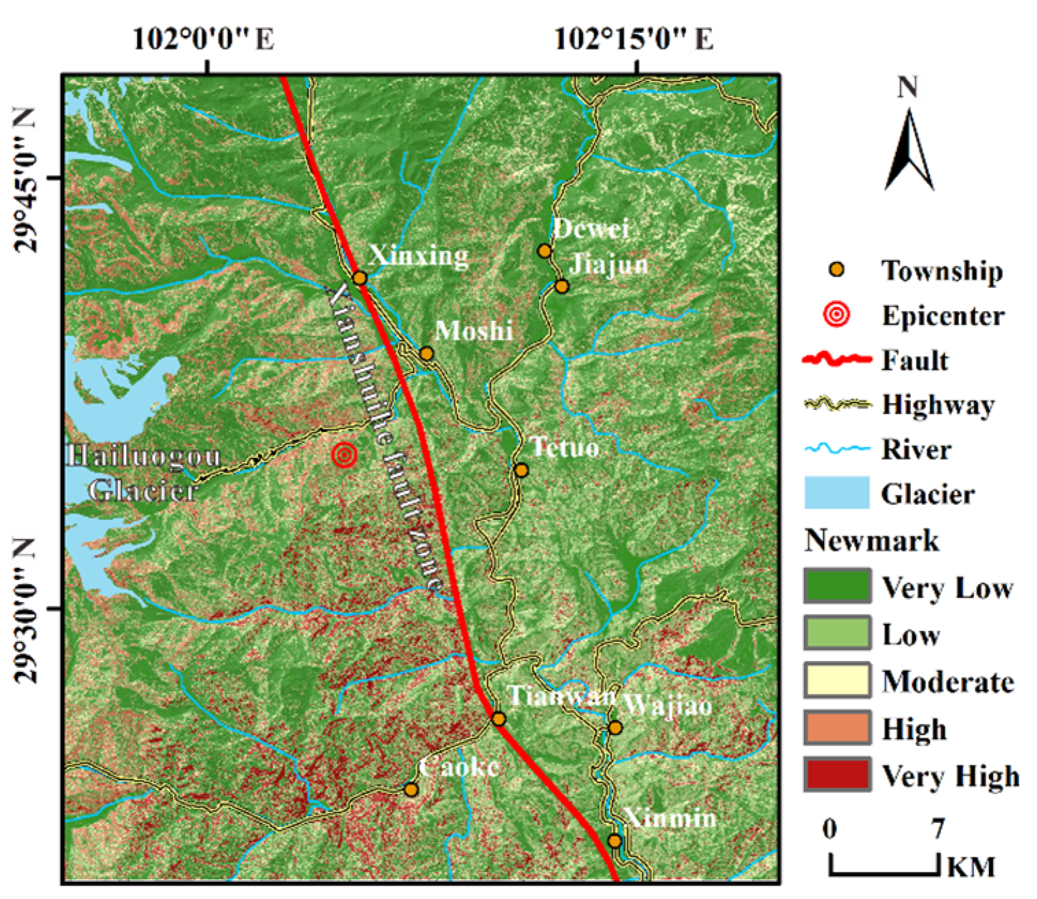
4.2. Evaluation of Earthquake-Induced Landslide Susceptibility Based on Newmark Physical Mechanics Model

The regional geological data at a scale of 1:500,000 were quickly collected to obtain the distribution map of engineering geological rock groups, as shown in Figure 8a. To ensure accurate slope values, a DEM (Digital Elevation Model) dataset with a resolution of 12.5 m was selected as the data source. The classification standards for engineering geological materials and the empirical values of engineering geological groups from both domestic and international sources were referenced. The parameter values are provided in Table 3. Considering that earthquake-induced landslides typically involve shallow slope failures, a nominal thickness of t = 2.5   m was adopted for the landslide thickness. The distribution of the static stability coefficient of the slope is calculated according to Equation (4) (see Figure 8b). In the process of calculating F s , the value for F s is obtained as <1 (meaning that it is unstable before the occurrence of the earthquake). In order to solve this problem, the region where the static coefficient F s < 1 is set to 1.01, referring to the research results of Dreyfus D et al. [38], so that the subsequent work can be carried out. The critical acceleration distribution is calculated according to Equation (3) and the static stability coefficient and slope data of the study area (see Figure 8c). The classic Newmark method involves the seismic acceleration time function, which is limited by the number of seismic stations and the number of strong seismic records in practical application, and the classic Newmark method is inconvenient for direct use in earthquake-induced landslide hazard prediction calculations. Therefore, scholars at home and abroad have used historical observation data to form numerous permanent displacement models [2,39,40,41]. The simplified Newmark displacement model can estimate slide displacement values in the absence of ground shaking acceleration records, and it then effectively analyzes the stability of seismic slopes.
Combined with the characteristics of the Luding earthquake, it is an obvious near-fault earthquake. There are obvious fault effects in near-fault earthquakes, and Pulse-like ground motions have been observed in near-fault records with directivity focusing or fling effects [42]. Pulse-like ground motions have a significant influence on landslide initiation, especially in near-fault areas [40]. Therefore, the permanent displacement model established by Zhang et al. [40], which considers the pulse effect of ground shaking, is chosen.
log ( D N ) = 6.021 ( a c P G A ) + 9.363 ( a c P G A ) 2 11.921 ( a c P G A ) 3 + 5.54 ( a c P G A ) 4 0.558 × log ( P G A ) + 1.416 × log ( P G V ) 0.208
where P G A is the peak ground acceleration and PGV is the peak ground velocity.
The ground shaking dataset was obtained from 79 strong-motion stations (see Figure 8d) provided by the China Earthquake Data Center (https://www.cea.gov.cn/ (accessed on 5 April 2023)). The station data contained three components of peak acceleration in the north-south, east-west and up-down directions. The average P G A for the two horizontal components of each strong motion record was calculated, and the P G A distribution was plotted using the inverse distance-weighted interpolation method. The amplification effect of slope topography is an important cause of seismic instability on slopes, and this effect is often positively correlated with the occurrence of seismic landslides. The amplification effect increases as the slope gradient and slope height increase, and the general amplification factor is 0.9~1.5 [43]. To improve the accuracy of the model’s evaluation, the terrain amplification coefficients in this study were calculated with reference to Equation (9) [44,45], and the original P G A and P G V were multiplied by K to finally obtain Figure 8e,f.
{ φ 15 °   or   H 15   , K = 1 φ > 15 °   and   H   > 30   , K = 1.2 30 ° φ < 45 °   and   H   > 30   , K = 1.4 φ 45 °   and   H   60   , K = 1.6
where φ is the slope of the slope; H is the relative height difference of the terrain; and K is the terrain amplification factor.
The permanent displacement model based on Equation (8) was used to obtain the Newmark cumulative displacement distribution of earthquakes in the study area (Figure 9). The selection of the critical displacement is still controversial. In this paper, with reference to previous studies, the landslide displacement threshold is set at 15 cm [38,46], i.e., a landslide is considered to occur if it is greater than 15 cm, and five landslide susceptibility classes are also classified.

4.3. Evaluation of Earthquake-Induced Landslides Based on IDNPM

Remote sensing technology possesses unique advantages for acquiring large-scale surface information and efficiently detecting subtle changes in topography. By monitoring and analyzing the target area with high-resolution remote sensing data before an earthquake, unstable slope areas can be precisely located and identified. These unstable slopes are more susceptible to seismic forces and prone to landslide occurrences compared to other areas. Therefore, it is necessary to integrate remote sensing data into a new quantitative risk assessment system for landslides. The permanent displacement values computed by the Newmark model partially reflect the potential risk of post-earthquake instability in natural slopes, providing certain advantages in earthquake-induced landslide prediction. However, this approach is influenced by empirical models and geotechnical parameters, thereby revealing limitations in terms of accuracy in practical applications. Based on the aforementioned considerations, by combining the assessment results of both approaches using Equation (6), the results presented in Figure 10 are obtained.

4.4. Evaluation and Comparison of Results

Accuracy assessment is an important and necessary step for evaluating the prediction accuracy and comparing the performance of evaluation models [47,48]. It involves comparing the predicted results with the actual landslide occurrences and using a compiled inventory of earthquake-induced landslides (Chen et al. [16] for this study) as the reference data. Based on the interpretation of multisource optical remote sensing images before and after the earthquake, a total of 2692 landslides were identified. The elevation of each grid unit corresponding to the landslide area was calculated, and grid units with elevations higher than the median elevation were considered the landslide source area [39] (see Figure 10).

4.4.1. Qualitative Evaluation of Assessment Results

In Figure 10, the left image presents the landslide assessment results obtained from the Newmark-InSAR model. Overall, a large number of landslide areas are classified as high- and very-high-risk zones, showing good consistency between the interpreted landslides and the evaluation results. To further compare the assessment results and identify differences, three representative areas within the study region are selected for qualitative comparison. These areas are labeled A, B and C, corresponding to Heiluo Gou A, Wanggangping B and Caokexiang C, respectively, as indicated by the light yellow regions in Figure 10. The right image in Figure 10 shows the results of the Newmark-InSAR model (1), the Newmark model (2) and the InSAR deformation (3) for each of the selected areas.
(1)
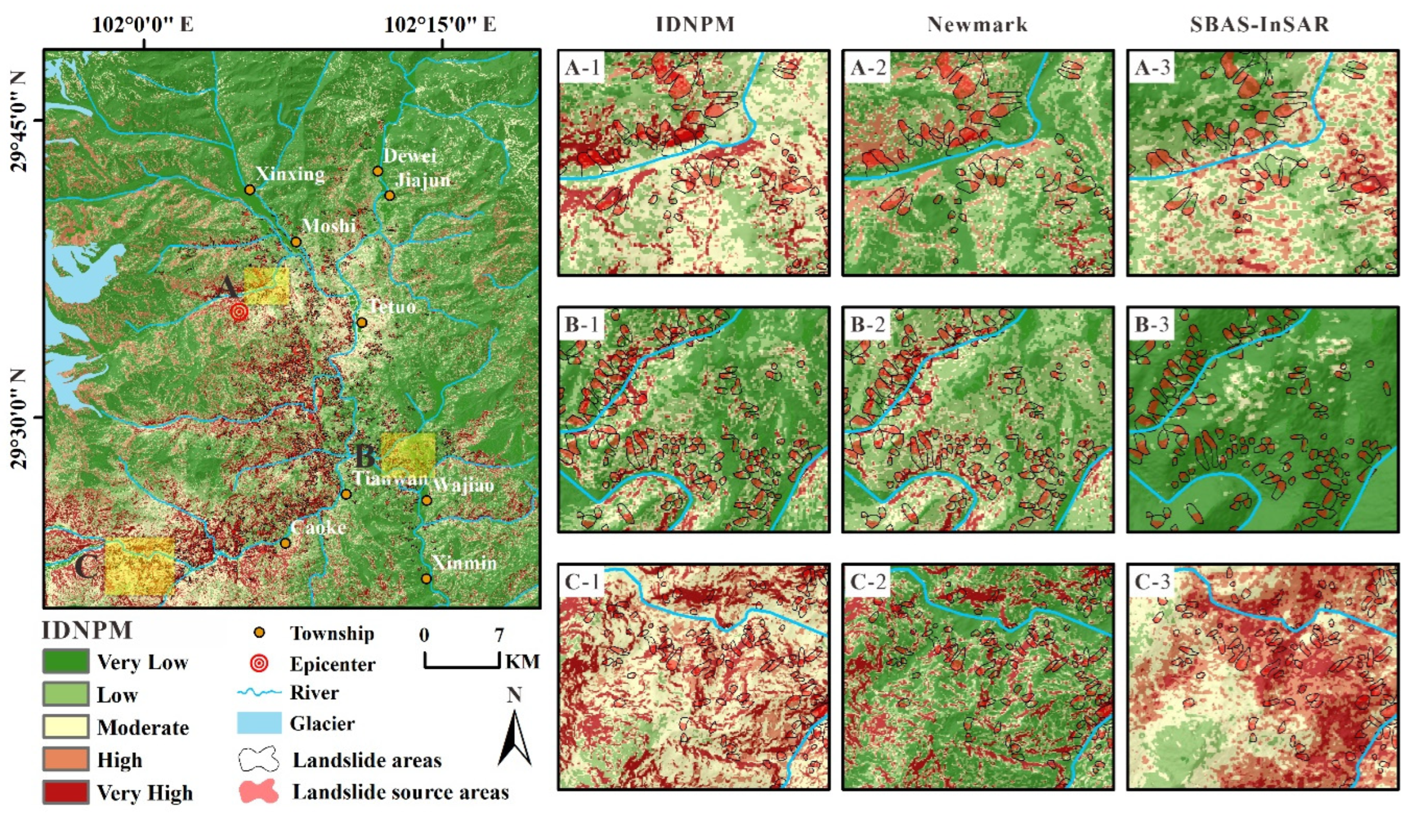
Hailuogou Glacier Forest Park in Gonggar Mountain is famous for its large, low-altitude modern glaciers and is also an important national protection area, and the epicenter of this earthquake was located in the park. The only road to the Hailuogou glacier scenic area is also located near the epicenter, so the typical area is set at the entrance A of the Hailuogou scenic area. Comparing the results of the three models, the highest agreement is found in the IDNPM, in which most of the triggered landslides are located in areas with higher hazards (redder color), and a large number of landslide source areas are more accurately located in areas with extremely high hazards. The reason for this is that the topographic data with 30 m resolution are somewhat coarse, resulting in errors in the prediction results; comparing the InSAR deformation results with the actual landslide distribution through A-3, it can reflect that there is a good correlation between landslide and pre-earthquake displacement. The larger deformation is mainly on both sides of the river bank, which shows large surface erosion and slow creeping deformation. Several small landslides in area A are in the area with large deformation, and the sensitivity of InSAR to the displacement of small landslides leads to improvements in the IDNPM’s accuracy.
(2)
Area B is at the mouth of the Hailiu River trench north of Wanggangping, which is also one of the concentrated development sites of these earthquake-induced landslides. Referring to the results of the PGA and PGV distribution in Figure 8, the seismic effect in area B is strong. The dynamic loading caused by the earthquake changes the stress distribution inside the landslide body, making the originally balanced landslide body subject to unbalanced forces, which leads to slope instability more easily in this area. The Newmark model fully considers the mechanism of earthquake landslide instability and strengthens the role of the seismic action and the slope’s own characteristics, so it has a better prediction performance in this area (see Figure 10B-2). The InSAR deformation data in B-3 reflect that there is no large deformation in this area before the earthquake, and they also corroborate that the landslide in this area is mainly initiated by this strong earthquake. With the master Newmark model, the IDNPM also maintains a high prediction accuracy in the B region.
(3)
The frequent occurrence of mudslides and floods in Cao Ke Township, Area C, combined with pre-earthquake deformation data (see Figure 10A), also reflects that there are more unstable slopes there. During the earthquake, the unstable slope was affected by both the direct impact of seismic waves and secondary effects induced by the earthquake, which further weakened its originally weaker stability. As a result, multiple earthquake-induced landslides occurred in the area during this earthquake. The terrain in this area is steep with strong topographic differences, and the main lithology is granite, which is classified as a hard rock group. In the prediction model of the Newmark model, it mainly shows that the danger zone is concentrated in the rugged area, and several small landslides in the gentle terrain are not accurately identified. However, the InSAR deformation data compensated for this deficiency, showing that several small landslides were already slipping before the earthquake, and the earthquake accelerated their slope movement. Combining the Newmark model’s results and pre-earthquake deformation data, the development of landslides can be predicted more accurately.

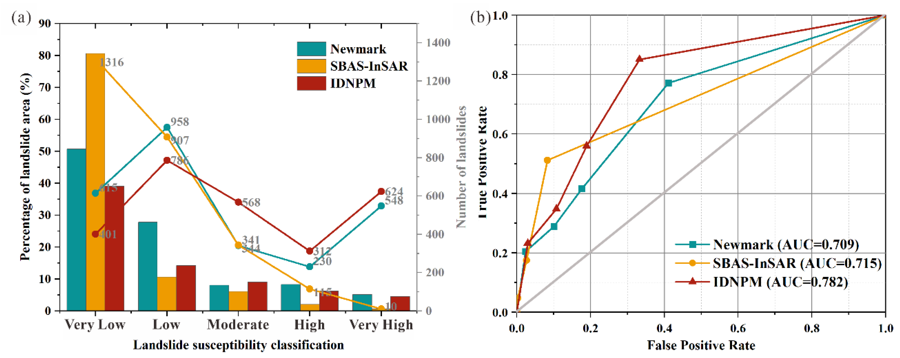
4.4.2. Quantitative Evaluation of Assessment Results

To accurately assess the predictive performance of the model, further quantitative analysis is required, and a confusion matrix [49] and Receiver Operating Characteristic (ROC) curves are the most important means to test the accuracy of the evaluation model in predicting geological hazard susceptibility [50]. The center of mass within the landslide source area was selected as the landslide source area, and an equal number of non-landslide points were also randomly selected within the study area as the data for this quantitative evaluation.
(1)
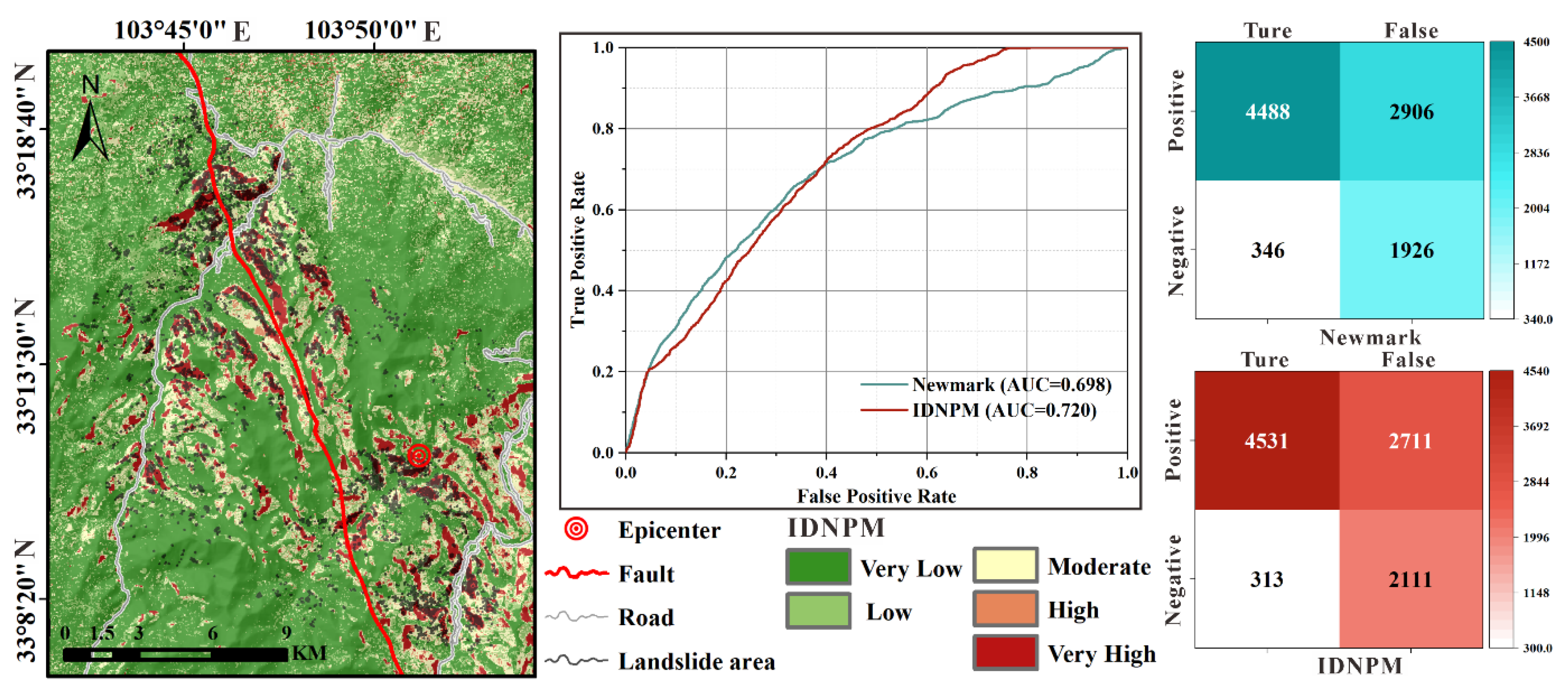
Quantitative analysis of the confusion matrix
The confusion matrix is a tool used to evaluate the performance of the classification model. According to the values of the confusion matrix in Figure 11, it is shown that the accuracy of true positives and true negatives in landslide disaster maps can be effectively improved, and false negative and false positive errors can be reduced to a certain extent by using the InSAR deformation based on the Newmark model.
To further quantify the performance of the model, the accuracy, precision, recall and F1-score of the model were calculated separately, and the results are presented in Table 4. It should be emphasized that the precision value indicates the percentage of successful landslide predictions, and these data indicate that the SBAS-InSAR deformation classification has a strong capability in accuracy. However, the precision value does not measure the overall prediction ability of the model alone, and its F1-score data reflect its poor overall performance in landslide predictions. Therefore, the SBAS-InSAR deformation classification cannot be directly used as the post-earthquake prediction result. In contrast, the reliability and overall performance of the conventional Newmark model are significantly better than the SBAS-InSAR deformation classification results, which also indicates that the InSAR deformation can only be in an auxiliary and corrective position in the IDNPM.
Compared with the traditional Newmark model, the prediction results based on the IDNPM achieved significant improvements in various indicators, with a 10.484% improvement in the accuracy value, a 6.410% improvement in the precision value, a 34.375% improvement in the recall value and a 22.414% improvement in the F1-score value. These data fully reflect that the IDNPM is significantly better than the traditional Newmark model in terms of performance.
(2)
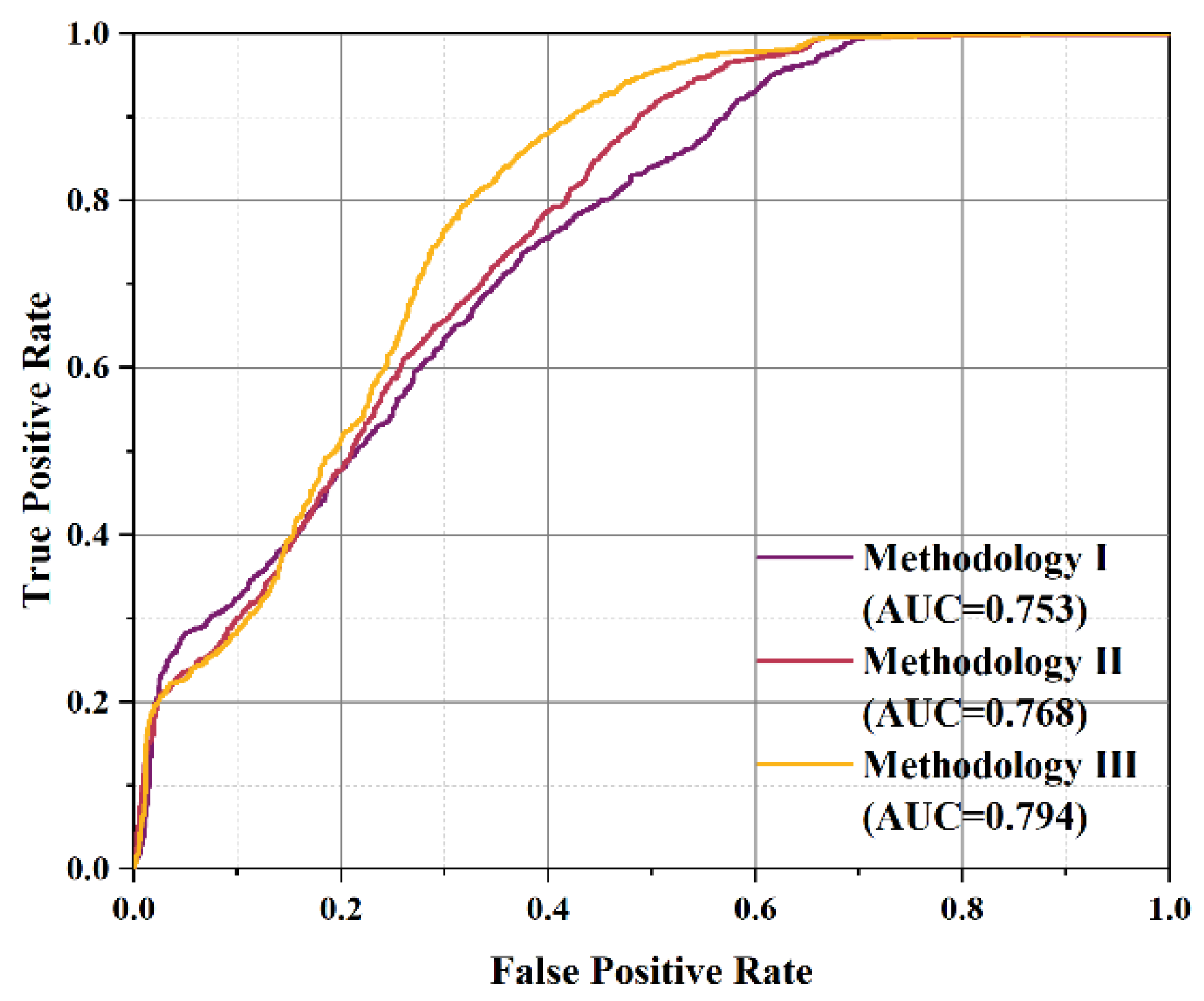
ROC curve quantitative analysis
The AUC value is the area enclosed by the ROC curve and the coordinate X-axis, and the general value is less than 1. The value closer to 1 indicates the higher accuracy of the model. Next, we use the ROC curve to further evaluate the classification ability and robustness of the model. First, the area percentage of each susceptibility class is calculated, and the number of landslide points in these classes is counted. The specific results are shown in Figure 12a. According to these data, we can observe that the corresponding area proportion gradually decreases with the increase in the susceptibility class. According to the number of landslide points, there are more landslide points and a higher landslide density in the high- and very-high-risk areas of the traditional Newmark model and IDNPM, which indicates that the overall prediction accuracy of these two models is higher. The ROC curve is then plotted, and the AUC value is calculated (see Figure 12b). The AUC value of the IDNPM is higher, with a gain of 10.296% compared to the conventional Newmark model. This gain is considerable, and in practical applications, 1% or 2% increments in accuracy control the final evaluation results of landslide susceptibility [51,52]. Also, we observed that the zoning result of SBAS-InSAR also has an AUC value of 0.715, which is slightly higher than that of the conventional Newmark method. However, according to the data in Figure 12a, it can also be found that a large number of landslide sites are not in the danger zone. Moreover, the combined analysis of the recall and F1-score values also confirms its weak performance in predicting landslides. The reason for the larger AUC value is that the SBAS-InSAR zoning is more accurate for non-landslides. Therefore, when assessing the accuracy of the landslide susceptibility model, there may be limitations based on the AUC values alone, and data such as the confusion matrix should be considered together for joint analysis and argumentation.
In summary, compared with the traditional Newmark model, the IDNPM introduces InSAR deformation data to complement natural slope features. InSAR technology provides more accurate landslide activity information by measuring surface deformation to accurately capture small changes in landslide slip. This makes the IDNPM a reliable method for post-earthquake landslide rapid emergency assessments, which has a high accuracy and can be used to more accurately study the development trend of landslides.

5. Discussion

5.1. Feasibility Study of IDNPM in Post-Earthquake Emergency Response

The objective of this study is to propose a model for post-earthquake landslide emergency assessments, mainly for emergency response guidance within 72 h after an earthquake. The overall construction of the IDNPM is simple, and electronic data from sources such as DEM, Sentinel-1A, Precise Orbit Determination, etc., in Table 1 are all pre-seismic data, which are freely available in various ways. Lithology data can be obtained from the local authorities or the National Geological Data Library, and ground shaking data can be obtained from the local seismic bureau or by using ShakeMap released by the USGS for calculation data. Lithology data can be obtained from local authorities or the National Geological Data Library, and ground shaking data can be obtained from the local seismological office when conditions permit. ShakeMap, published by the USGS, can also be used for calculation data. These data can be collected in a timely manner in the first hour after an earthquake. Rapid assessments based on Newmark model and specific calculations of SBAS-InSAR deformation monitoring can be completed within a few hours of receiving the emergency response task. In addition, via comparison with the same earthquake landslide list of the Luding earthquake, some performance indicators also prove the high prediction accuracy of the IDNPM, which can provide timely data support for post-earthquake emergency rescues.

5.2. Discussion on the Construction of IDNPM

Many data fusion methods currently exist [53,54], and complex data fusion methods place greater demands on the complexity and richness of the data. The IDNPM construction process proposed in this paper aims to be simple and effective, and thus, the weighted superposition method is directly chosen to achieve the organic integration of Newmark model and InSAR deformation data. However, such an approach ignores the differences and correlations between the two, and the weights are currently assigned only with reference to empirical values. Therefore, the results obtained are inevitably biased, and it is necessary to further explore the IDNPM construction method. Thus, the following three options are applied to try to bring out the optimal performance of the model.
Methodology I: A larger pre-seismic deformation rate means poorer landslide stability. Therefore, the following are considered: combining the deformation classification of InSAR; setting different FS discount factors; and correcting the static safety factor according to the discount factor K1. Levels from very low to very high correspond to K1 = 1, 0.9, …, 0.6, respectively. The modified FS is then used to obtain the evaluation results of earthquake landslide susceptibility.
Methodology Ⅱ: A higher pre-seismic deformation rate implies that the landslide already had a certain amount of displacement before the earthquake, so different displacement amplification factors were considered in combination with the InSAR deformation classification. The accumulated displacement values obtained by the Newmark method are corrected according to the amplification factor K2, and levels from very low to very high correspond to K2 = 1, 1.1, …, 1.4, respectively. Using the corrected Dn values, the evaluation results of earthquake landslide susceptibility are obtained again.
Methodology Ⅲ: Also, for the discussion on the displacement amount, this program directly uses the one-year cumulative displacement of the deformation rate of InSAR as the data base. Combined with the analysis results in Section 4.4.2, the InSAR deformation can only be in an auxiliary and corrective position in the IDNPM model. Thus, 0.5 times the InSAR displacement is taken for comparison with the Newmark cumulative displacement, and the maximum value in the two raster data is taken to regain the results for earthquake-induced landslide susceptibility evaluation.
The ROC curves and AUC value results of Figure 13 were obtained, and the results of the study show that the models constructed with the three schemes had different accuracies with slight differences, which indicated that the rationality of the construction method played a key role in the final prediction results. Among them, the IDNPM model constructed with Methodology Ⅲ shows the best performance, which indicates that the correlation between the InSAR-shaped variables and the Dn values of Newmark needs to be further explored to uncover the relationship between them. Combining the results obtained with the three schemes and the scheme used in this paper, the accuracy of the weight superposition method used in this paper also reaches a superior level, which is comparable to the results of Methodology Ⅲ. Therefore, in the future, if the correlation law between the pre-seismic shape variables and the permanent displacement of Newmark is not obtained in similar seismic events, the construction method used in this paper can be directly adopted for the rapid emergency assessment of post-earthquake landslides in the IDNPM.

5.3. Generalization Performance Analysis of IDNPM

To evaluate the reliability of the IDNPM in the face of arbitrary seismic events, it is therefore necessary to test the generalization performance of the model. We chose the 7.0 magnitude earthquake that occurred in Jiuzhaigou County on 8 August 2017, which caused property damage of up to 1.58 billion yuan, as a test case. Following the IDNPM construction process described in Section 2.3, we first acquired pre-earthquake multi-temporal remote sensing images and then used the Newmark model to perform a rapid assessment, which finally resulted in the post-earthquake landslide susceptibility evaluation results (see Figure 14). To verify the accuracy of the model, we used a confusion matrix and ROC curve for analysis. According to the data in Figure 14, the AUC value of the conventional Newmark method in the Jiuzhaigou area is 0.698, and the accuracy is improved by 3.152% after the introduction of InSAR deformation data. The performance indexes calculated with the confusion matrix reflect that the model has a good classification ability overall. Combining the performance metrics obtained from the confusion matrix calculation (see Table 5), it can be found that the model has an overall better classification capability. According to the results, the performance of the IDNPM model has been optimized to a certain extent after the introduction of InSAR deformation data. However, it is also found that the IDNPM does not achieve higher accuracy. The reason for this analysis is that the Jiuzhaigou synoptic landslide is mainly developed in dense vegetation and snow-covered areas, and seasonal snowmelt and dense vegetation can lead to low coherence and decoherence phenomena. This then leads to the failure of InSAR technology to detect subtle changes in terrain prior to earthquakes, which limits the prediction ability of the IDNPM.

5.4. Analysis of Limitations and Improvements for IDNPM

This study clearly demonstrates significant accuracy improvements in the IDNPM (Newmark-InSAR Model) compared to the traditional Newmark model. However, there are still some limitations and areas for future improvement. First, landslides often occur in steep valleys with significant topographic variations. SAR (Synthetic Aperture Radar) systems have a side-looking imaging geometry, which introduces geometric distortions such as layover, foreshortening and shadow effects. These geometric distortions severely affect the capability of SAR for monitoring surface deformations, leading to observation failures and inconsistent deformation results between ascending and descending orbits. Using data from either the ascending or descending orbit alone to detect potential landslides has significant limitations, as both geometric distortions and slope gradients can influence LOS (Line of Sight) displacement measurements [55]. Therefore, for future IDNPM construction, it is recommended to obtain surface deformation rates from the satellite operating in different orbits (ascending and descending) to address the issue of undetected landslide activity. Furthermore, landslides occurring in glacier-covered or vegetation-active areas pose challenges for SAR interpretation. Complex surface activities and the presence of vegetation or glacier cover can cause decorrelation in SAR images, making it difficult to accurately identify unstable slopes. Addressing these situations requires more advanced processing algorithms and models. Last, the IDNPM model was constructed in this study to be simple and effective, relying only on empirical weightings combined with the Newmark model and InSAR deformation data. Although it achieved promising accuracy improvements, the model still lacks theoretical support. Therefore, future research should carefully consider the differences and correlations between the two methods to further enhance the accuracy and stability of IDNPM assessment results.

6. Conclusions

This study aims to address the needs of post-earthquake emergency responses by proposing a methodology that combines remote sensing technology and the Newmark rapid landslide assessment model. The objective is to improve the accuracy and precision of post-earthquake landslide predictions. First, remote sensing technology is employed to successfully identify unstable slopes in the geological environment. These unstable slopes are more susceptible to seismic forces and more prone to landslides compared to other areas. Second, the Newmark model is applied for the rapid assessment of landslides in the study area. Based on mechanical principles, the Newmark model is sensitive to seismic parameters and slope characteristics, taking into account the mechanisms of landslide instability and providing more accurate quantitative values of landslide displacements. Last, these two methods are organically combined, and the dynamic deformation of the ground surface and geological features are comprehensively considered to finally obtain the IDNPM landslide prediction and assessment results.
Taking the 5 September 2022 Luding earthquake as an example, the research results demonstrate that IDNPM effectively reduces false negatives and false positives in landslide predictions by utilizing SAR deformation information, thus improving the accuracy and reliability of landslide predictions. Compared with the traditional Newmark model, the accuracy of the IDNPM is improved by about 10%. Applying the IDNPM to the 8 August 2017 Jiuzhaigou earthquake, the prediction accuracy is improved by 3.152%, which also reflects that the IDNPM has good generalization performance. Furthermore, the IDNPM is simple and convenient to implement and exhibits high reliability and precision. We expect that the findings of this study will serve as an important reference for future earthquake-induced landslide emergency prediction models. The landslide emergency assessment results obtained through the IDNPM can provide timely information on the macro-distribution of landslides, offering robust data support for post-disaster emergency responses and recovery efforts in affected areas.

Author Contributions

Y.Z. (Ying Zeng): Methodology, Drawing, Writing—original draft preparation, Writing—review and editing. Y.Z. (Yingbin Zhang): Conceptualization, Supervision, Writing—review and editing, Funding acquisition. J.L.: Writing—review and editing. Q.W.: Writing—review and editing. H.Z.: Writing—review and editing. All authors have read and agreed to the published version of the manuscript.

Funding

This study was financially supported by the National Natural Science Foundation of China (52378370, 41977213, 52278372), The Second Tibetan Plateau Scientific Expedition and Research Program (STEP) (2019QZKK0906) and The National Ten Thousand Talent Program for Young Top-notch Talents, China Road & Bridge Corporation (P220447). Their financial support is gratefully acknowledged.

Conflicts of Interest

The authors declare that they have no known competing financial interests or personal relationships that could have appeared to influence the work reported in this paper.

References

  1. Julian, J.B.; Carlos, E.R. Earthquake-Induced Landslides in Central America. Eng. Geol. 2002, 63, 189–220. [Google Scholar] [CrossRef]
  2. Jibson, R.W. Regression Models for Estimating Coseismic Landslide Displacement. Eng. Geol. 2007, 91, 209–218. [Google Scholar] [CrossRef]
  3. Koronovskii, N.V.; Zakharov, V.S.; Naimark, A.A. The Unpredictability of Strong Earthquakes: New Understanding and Solution of the Problem. Mosc. Univ. Geol. Bull. 2021, 76, 366–373. [Google Scholar] [CrossRef]
  4. Xi, C. Effectiveness of Newmark-Based Sampling Strategy for Coseismic Landslide Susceptibility Mapping Using Deep Learning, Support Vector Machine, and Logistic Regression. Bull. Eng. Geol. Environ. 2022, 81, 208. [Google Scholar] [CrossRef]
  5. Gallen, S.F.; Clark, M.K.; Godt, J.W.; Roback, K.; Niemi, N.A. Application and Evaluation of a Rapid Response Earthquake-Triggered Landslide Model to the 25 April 2015 Mw 7.8 Gorkha Earthquake, Nepal. Tectonophysics 2016, 714–715, 173–187. [Google Scholar] [CrossRef]
  6. Guzzetti, F.; Mondini, A.C.; Cardinali, M.; Fiorucci, F.; Santangelo, M.; Chang, K.-T. Landslide Inventory Maps: New Tools for an Old Problem. Earth-Sci. Rev. 2012, 112, 42–66. [Google Scholar] [CrossRef]
  7. Fan, X.; Scaringi, G.; Xu, Q.; Zhan, W.; Dai, L.; Li, Y.; Pei, X.; Yang, Q.; Huang, R. Coseismic Landslides Triggered by the 8th August 2017 Ms 7.0 Jiuzhaigou Earthquake (Sichuan, China): Factors Controlling Their Spatial Distribution and Implications for the Seismogenic Blind Fault Identification. Landslides 2018, 15, 967–983. [Google Scholar] [CrossRef]
  8. Fan, X.; Wang, X.; Dai, L.; Fang, C.; Deng, Y.; Zou, C.; Tang, M.; Wei, Z.; Dou, X.; Zhang, J.; et al. Characteristics and spatial distribution pattern of Ms 6.8 Luding earthquake occurred on September 5, 2022. J. Eng. Geol. 2022, 30, 1504–1516. [Google Scholar] [CrossRef]
  9. Liu, J.; Wang, T.; Du, J.; Chen, K.; Huang, J.; Wang, H.; Ruan, Q.; Feng, F. Emergency rapid assessment of landslides induced by the Luding Ms6.8 earthquake in Sichuan of China. Hydrogeol. Eng. Geol. 2023, 50, 84–94. [Google Scholar] [CrossRef]
  10. Du, Q.; Chen, D.; Li, G.; Cao, Y.; Zhou, Y.; Chai, M.; Wang, F.; Qi, S.; Wu, G.; Gao, K.; et al. Preliminary Study on InSAR-Based Uplift or Subsidence Monitoring and Stability Evaluation of Ground Surface in the Permafrost Zone of the Qinghai–Tibet Engineering Corridor, China. Remote Sens. 2023, 15, 3728. [Google Scholar] [CrossRef]
  11. Han, Y.; Li, T.; Dai, K.; Lu, Z.; Yuan, X.; Shi, X.; Liu, C.; Wen, N.; Zhang, X. Revealing the Land Subsidence Deceleration in Beijing (China) by Gaofen-3 Time Series Interferometry. Remote Sens. 2023, 15, 3665. [Google Scholar] [CrossRef]
  12. Gao, H.; Gao, Y.; Li, B.; Yin, Y.; Yang, C.; Wan, J.; Zhang, T. The Dynamic Simulation and Potential Hazards Analysis of the Yigong Landslide in Tibet, China. Remote Sens. 2023, 15, 1322. [Google Scholar] [CrossRef]
  13. Wang, Y.; Cui, X.; Che, Y.; Li, P.; Jiang, Y.; Peng, X. Identification and Analysis of Unstable Slope and Seasonal Frozen Soil Area along the Litang Section of the Sichuan–Tibet Railway, China. Remote Sens. 2023, 15, 1317. [Google Scholar] [CrossRef]
  14. Liang, R.; Dai, K.; Shi, X.; Guo, B.; Dong, X.; Liang, F.; Tomás, R.; Wen, N.; Fan, X. Automated Mapping of Ms 7.0 Jiuzhaigou Earthquake (China) Post-Disaster Landslides Based on High-Resolution UAV Imagery. Remote Sens. 2021, 13, 1330. [Google Scholar] [CrossRef]
  15. Zhang, P.; Xu, C.; Ma, S.; Shao, X.; Tian, Y.; Wen, B. Automatic Extraction of Seismic Landslides in Large Areas with Complex Environments Based on Deep Learning: An Example of the 2018 Iburi Earthquake, Japan. Remote Sens. 2020, 12, 3992. [Google Scholar] [CrossRef]
  16. Chen, B.; Li, Z.; Huang, W.; Liu, Z.; Zhang, C.; Du, J.; Song, C.; Ding, M.; Zhu, W.; Zhang, S.; et al. Spatial Distribution and influencing Factors of Geohazards induced by the 2022 M6.6 Luding (Sichuan, China) Earthouake. J. Earth Sci. Environ. 2022, 44, 971–985. [Google Scholar] [CrossRef]
  17. Zhuo, Y.-Q.; Liu, P.; Guo, Y.; Chen, H.; Chen, S.; Wang, K. Cross-Effects of Loading Rate and Cumulative Fault Slip on Pre-Seismic Rupture and Unstable Slip Rate of Laboratory Earthquakes. Tectonophysics 2022, 826, 229266. [Google Scholar] [CrossRef]
  18. Chen, X.; Liu, C.; Wang, M. A Method for Quick Assessment of Earthquake-Triggered Landslide Hazards: A Case Study of the Mw6.1 2014 Ludian, China Earthquake. Bull. Eng. Geol. Environ. 2018, 78, 2449–2458. [Google Scholar] [CrossRef]
  19. Ji, J.; Wang, C.; Cui, H.; Li, X.; Gao, Y. A Simplified Nonlinear Coupled Newmark Displacement Model with Degrading Yield Acceleration for Seismic Slope Stability Analysis. Int. J. Numer. Anal. Methods Geomech. 2021, 45, 1303–1322. [Google Scholar] [CrossRef]
  20. Berardino, P.; Fornaro, G.; Lanari, R.; Sansosti, E. A New Algorithm for Surface Deformation Monitoring Based on Small Baseline Differential SAR Interferograms. IEEE Trans. Geosci. Remote Sens. 2002, 40, 2375–2383. [Google Scholar] [CrossRef]
  21. Parise, M.; Jibson, R.W. A Seismic Landslide Susceptibility Rating of Geologic Units Based on Analysis of Characteristics of Landslides Triggered by the 17 January, 1994 Northridge, California Earthquake. Eng. Geol. 2000, 58, 251–270. [Google Scholar] [CrossRef]
  22. Cao, C.; Zhu, K.; Xu, P.; Shan, B.; Yang, G.; Song, S. Refined Landslide Susceptibility Analysis Based on InSAR Technology and UAV Multi-Source Data. J. Clean. Prod. 2022, 368, 133146. [Google Scholar] [CrossRef]
  23. Devara, M.; Tiwari, A.; Dwivedi, R. Landslide Susceptibility Mapping Using MT-InSAR and AHP Enabled GIS-Based Multi-Criteria Decision Analysis. Geomat. Nat. Hazards Risk 2021, 12, 675–693. [Google Scholar] [CrossRef]
  24. Ciampalini, A.; Raspini, F.; Lagomarsino, D.; Catani, F.; Casagli, N. Landslide Susceptibility Map Refinement Using PSInSAR Data. Remote Sens. Environ. 2016, 184, 302–315. [Google Scholar] [CrossRef]
  25. Zhang, Y.; Deng, L.; Han, Y.; Sun, Y.; Zang, Y.; Zhou, M. Landslide Hazard Assessment in Highway Areas of Guangxi Using Remote Sensing Data and a Pre-Trained XGBoost Model. Remote Sens. 2023, 15, 3350. [Google Scholar] [CrossRef]
  26. Fan, X.; Yunus, A.P.; Scaringi, G.; Catani, F.; Siva Subramanian, S.; Xu, Q.; Huang, R. Rapidly Evolving Controls of Landslides After a Strong Earthquake and Implications for Hazard Assessments. Geophys. Res. Lett. 2021, 48, 509. [Google Scholar] [CrossRef]
  27. Wang, X.; Fang, C.; Tang, X.; Dai, L.; Fan, X.; Xu, Q. Research on Emergency Evaluation of L.andslides Induced bythe L.uding Ms 6.8 Earthquake. Geomat. Inf. Sci. Wuhan Univ. 2023, 48, 25–35. [Google Scholar] [CrossRef]
  28. Sun, D.; Yang, T.; Cao, N.; Qin, L.; Hu, X.; Wei, M.; Meng, M.; Zhang, W. Characteristics and Prevention of Coseismic Geohazard Induced by Luding Ms 6.8 Earthquake, Sichuan, China. Earth Sci. Front. 2023, 30, 476–493. [Google Scholar] [CrossRef]
  29. Wang, X.; Fan, X.; Xu, Q.; Du, P. Change Detection-Based Co-Seismic Landslide Mapping through Extended Morphological Profiles and Ensemble Strategy. ISPRS J. Photogramm. Remote Sens. 2022, 187, 225–239. [Google Scholar] [CrossRef]
  30. Cascini, L.; Fornaro, G.; Peduto, D. Advanced Low- and Full-Resolution DInSAR Map Generation for Slow-Moving Landslide Analysis at Different Scales. Eng. Geol. 2010, 112, 29–42. [Google Scholar] [CrossRef]
  31. Dai, C.; Li, W.; Lu, H.; Zhang, S. Landslide Hazard Assessment Method Considering the Deformation Factor: A Case Study of Zhouqu, Gansu Province, Northwest China. Remote Sens. 2023, 15, 596. [Google Scholar] [CrossRef]
  32. Herrera, G.; Gutiérrez, F.; García-Davalillo, J.C.; Guerrero, J.; Notti, D.; Galve, J.P.; Fernández-Merodo, J.A.; Cooksley, G. Multi-Sensor Advanced DInSAR Monitoring of Very Slow Landslides: The Tena Valley Case Study (Central Spanish Pyrenees). Remote Sens. Environ. 2013, 128, 31–43. [Google Scholar] [CrossRef]
  33. Aslan, G.; Foumelis, M.; Raucoules, D.; De Michele, M.; Bernardie, S.; Cakir, Z. Landslide Mapping and Monitoring Using Persistent Scatterer Interferometry (PSI) Technique in the French Alps. Remote Sens. 2020, 12, 1305. [Google Scholar] [CrossRef]
  34. Novellino, A.; Cesarano, M.; Cappelletti, P.; Di Martire, D.; Di Napoli, M.; Ramondini, M.; Sowter, A.; Calcaterra, D. Slow-Moving Landslide Risk Assessment Combining Machine Learning and InSAR Techniques. CATENA 2021, 203, 105317. [Google Scholar] [CrossRef]
  35. Zhou, C.; Cao, Y.; Hu, X.; Yin, K.; Wang, Y.; Catani, F. Enhanced Dynamic Landslide Hazard Mapping Using MT-InSAR Method in the Three Gorges Reservoir Area. Landslides 2022, 19, 1585–1597. [Google Scholar] [CrossRef]
  36. Kouhartsiouk, D.; Perdikou, S. The Application of DInSAR and Bayesian Statistics for the Assessment of Landslide Susceptibility. Nat. Hazards 2021, 105, 2957–2985. [Google Scholar] [CrossRef]
  37. Casagli, N.; Intrieri, E.; Tofani, V.; Gigli, G.; Raspini, F. Landslide Detection, Monitoring and Prediction with Remote-Sensing Techniques. Nat. Rev. Earth Environ. 2023, 4, 51–64. [Google Scholar] [CrossRef]
  38. Dreyfus, D.; Rathje, E.M.; Jibson, R.W. The Influence of Different Simplified Sliding-Block Models and Input Parameters on Regional Predictions of Seismic Landslides Triggered by the Northridge Earthquake. Eng. Geol. 2013, 163, 41–54. [Google Scholar] [CrossRef]
  39. Jibson, R.W.; Harp, E.L.; Michael, J.A. A Method for Producing Digital Probabilistic Seismic Landslide Hazard Maps. Eng. Geol. 2000, 58, 271–289. [Google Scholar] [CrossRef]
  40. Zhang, Y.; Liu, J.; Cheng, Q.; Xiao, L.; Zhao, L.; Xiang, C.; Buah, P.A.; Yu, H.; He, Y. A New Permanent Displacement Model Considering Pulse-like Ground Motions and Its Application in Landslide Hazard Assessment. Soil Dyn. Earthq. Eng. 2022, 163, 107556. [Google Scholar] [CrossRef]
  41. Liu, J.; Fu, H.; Zhang, Y.; Xu, P.; Hao, R.; Yu, H.; He, Y.; Deng, H.; Zheng, L. Effects of the Probability of Pulse-like Ground Motions on Landslide Susceptibility Assessment in near-Fault Areas. J. Mt. Sci. 2023, 20, 31–48. [Google Scholar] [CrossRef]
  42. Moustafa, A.; Takewaki, I. Characterization and Modeling of Near-Fault Pulse-like Strong Ground Motion via Damage-Based Critical Excitation Method. Struct. Eng. Mech. 2010, 34, 755–778. [Google Scholar] [CrossRef]
  43. Du, G.; Zhang, Y.; Yang, Z.; Iqbal, J.; Tong, B.; Guo, C.; Yao, X.; Wu, R. Estimation of Seismic Landslide Hazard in the Eastern Himalayan Syntaxis Region of Tibetan Plateau. Acta Geol. Sin.-Engl. Ed. 2017, 91, 658–668. [Google Scholar] [CrossRef]
  44. Zhao, H.; Ma, F.; Li, Z.; Guo, J.; Zhang, J. Optimization of parameters and application of probabilistic seismiclandslide hazard analysis model based on Newmark displacement model: A case study in Ludian earthquake area. Earth Sci. 2022, 47, 4401–4416. [Google Scholar] [CrossRef]
  45. Rodríguez-Peces, M.J.; García-Mayordomo, J.; Azañón, J.M.; Jabaloy, A. GIS Application for Regional Assessment of Seismically Induced Slope Failures in the Sierra Nevada Range, South Spain, along the Padul Fault. Environ. Earth Sci. 2014, 72, 2423–2435. [Google Scholar] [CrossRef]
  46. Liu, J.; Zhang, Y.; Wei, J.; Xiang, C.; Wang, Q.; Xu, P.; Fu, H. Hazard Assessment of Earthquake-Induced Landslides by Using Permanent Displacement Model Considering near-Fault Pulse-like Ground Motions. Bull. Eng. Geol. Environ. 2021, 80, 8503–8518. [Google Scholar] [CrossRef]
  47. Cantarino, I.; Carrion, M.A.; Goerlich, F.; Ibaez, V.M. A ROC Analysis-Based Classification Method for Landslide Susceptibility Maps. Landslides 2019, 16, 265–282. [Google Scholar] [CrossRef]
  48. Song, Y.; Niu, R.; Xu, S.; Ye, R.; Peng, L.; Guo, T.; Li, S.; Chen, T. Landslide Susceptibility Mapping Based on Weighted Gradient Boosting Decision Tree in Wanzhou Section of the Three Gorges Reservoir Area (China). Int. J. Geo-Inf. 2018, 8, 4. [Google Scholar] [CrossRef]
  49. Landis, J.R.; Koch, G.G. The Measurement of Observer Agreement for Categorical Data. Biometrics 1977, 33, 159–174. [Google Scholar] [CrossRef] [PubMed]
  50. Chung, C.-J.; Fabbri, A.G. Predicting Landslides for Risk Analysis—Spatial Models Tested by a Cross-Validation Technique. Geomorphology 2008, 94, 438–452. [Google Scholar] [CrossRef]
  51. Pradhan, B. A Comparative Study on the Predictive Ability of the Decision Tree, Support Vector Machine and Neuro-Fuzzy Models in Landslide Susceptibility Mapping Using GIS. Comput. Geosci. 2013, 51, 350–365. [Google Scholar] [CrossRef]
  52. Jebur, M.; Pradhan, B.; Tehrany, M. Optimization of Landslide Conditioning Factors Using Very High-Resolution Airborne Laser Scanning (LiDAR) Data at Catchment Scale. Remote Sens. Environ. 2014, 152, 150–165. [Google Scholar] [CrossRef]
  53. Mitchell, H. Data Fusion: Concepts and Ideas; Springer: Berlin, Germany, 2012; pp. 125–142. ISBN 978-3-642-27221-9. [Google Scholar]
  54. Stankevich, S.; Titarenko, O.; Svideniuk, M. Landslide Susceptibility Mapping Using GIS-Based Weight-of-Evidence Modelling in Central Georgian Regions. In Proceedings of the Natural Disasters in Georgia: Monitoring, Prevention, Mitigation, Tbilisi, Georgia, 12 December 2019; pp. 187–190. [Google Scholar]
  55. Dai, K.; Deng, J.; Xu, Q.; Li, Z.; Shi, X.; Hancock, C.; Wen, N.; Zhang, L.; Zhuo, G. Interpretation and Sensitivity Analysis of the InSAR Line of Sight Displacements in Landslide Measurements. GISci. Remote Sens. 2022, 59, 1226–1242. [Google Scholar] [CrossRef]
Figure 1. IDNPM construction process.
Remotesensing 15 04605 g001
Figure 2. Location and topographic map of the study area.
Remotesensing 15 04605 g002
Figure 3. Sentinel image coverage map.
Remotesensing 15 04605 g003
Figure 4. (a) Image spatial baseline; (b) Image time baseline.
Remotesensing 15 04605 g004
Figure 5. Radar line of sight to geometric relationship diagram [30].
Remotesensing 15 04605 g005
Figure 6. SBAS-InSAR deformation rate: (a) LOS direction; (b) Steepest direction of slope; (c) Steepest direction of slope after correction.
Remotesensing 15 04605 g006
Figure 7. Results of surface deformation zoning: (a) SBAS-InSAR landslide susceptibility classification results; (b) Comparison of SBAS-InSAR and Newmark method area percentages for each zoning class.
Remotesensing 15 04605 g007
Figure 8. Newmark correlation analysis diagram: (a) Geological map of the study area; (b) FS distribution; (c) Ac distribution; (d) Distribution of strong-motion recording stations; (e) PGA distribution; (f) PGV distribution.
Remotesensing 15 04605 g008
Figure 9. Newmark model landslide susceptibility classification results.
Remotesensing 15 04605 g009
Figure 10. IDNPM landslide susceptibility evaluation results: (A-1) IDNPM evaluation results in region A; (B-1) IDNPM evaluation results in region B; (C-1) IDNPM evaluation results in region C; (A-2) Newmark model evaluation results in region A; (B-2) Newmark model evaluation results in region B; (C-2) Newmark model evaluation results in region C; (A-3) SBAS-InSAR method evaluation results in region A; (B-3) SBAS-InSAR method evaluation results in region B; (C-3) SBAS-InSAR method evaluation results in region C.
Remotesensing 15 04605 g010
Figure 11. Confusion matrix comparison plot.
Remotesensing 15 04605 g011
Figure 12. Comparison of quantitative analysis of evaluation models: (a) Percentage of area in each susceptibility class and number of landslides; (b) ROC curves and AUC values of each model.
Remotesensing 15 04605 g012
Figure 13. ROC curves and AUC values of each model: Methodology I involves the setting of various static safety discount factors; Methodology II focuses on setting the displacement amplification factor; and Methodology III considers the annual cumulative deformation value.
Remotesensing 15 04605 g013
Figure 14. Jiuzhaigou IDNPM landslide evaluation results and model prediction accuracy results.
Remotesensing 15 04605 g014
Table 1. Data and sources used.
Data NameData ScaleData PhaseData Source
Sentinel-1A5 m × 20 mAugust 2021–August 2022Alaska Satellite Facility (ASF) https://search.asf.alaska.edu (accessed on 21 March 2023)
Precise Orbit Determination-August 2021–August 2022European Space Agency https://scihub.copernicus.eu (accessed on 21 March 2023)
DEM12.5 m2011Alaska Satellite Facility (ASF) https://search.asf.alaska.edu (accessed on 20 March 2023)
DEM30 m2021Japan Aerospace Exploration Agency https://global.jaxa.jp (accessed on 20 March 2023)
Lithology1:500,0002013National Geological Data Library
http://www.ngac.org.cn (accessed on 6 September 2022)
Seismic station data-2022China Earthquake Administration
https://www.cea.gov.cn/ (accessed on 5 April 2023)
Google satellite image0.5 m2022Google earth software
https://earth.google.com (accessed on 21 March 2023)
Table 2. Surface deformation rate classification rules.
ClassificationsVery LowLowModerateHighVery High
V S l o p e (mm/a)<3.0123.012–7.3417.341–11.67111.671–16.0≥16.0
Table 3. Values of lithological mechanical parameters in the study area.
IDEngineering Geological Units c ( k P a ) φ ( ° )
1Hard rock2734
2Relatively hard rock Ⅰ2330
3Relatively hard rock Ⅱ2229
4Relatively soft rock2027
5Soft Rock1926
Table 4. Comparison of model performance metrics (Three models).
Prediction PerformancePrediction Models
NewmarkSBAS-InSARIDNPM
Accuracy0.6200.5740.685
Precision0.7020.8690.747
Recall0.4160.1750.559
F1-score0.5220.2910.639
Table 5. Comparison of model performance metrics (Two models).
Prediction PerformancePrediction Models
NewmarkIDNPM
Accuracy0.6630.687
Precision0.6070.626
Recall0.9280.935
F1-score0.7340.750
Disclaimer/Publisher’s Note: The statements, opinions and data contained in all publications are solely those of the individual author(s) and contributor(s) and not of MDPI and/or the editor(s). MDPI and/or the editor(s) disclaim responsibility for any injury to people or property resulting from any ideas, methods, instructions or products referred to in the content.

