Article

Land Subsidence Prediction and Analysis along Typical High-Speed Railways in the Beijing–Tianjin–Hebei Plain Area

1
Key Laboratory of the Ministry of Education Land Subsidence Mechanism and Prevention, Capital Normal University, Beijing 100048, China
2
College of Resources Environment and Tourism, Capital Normal University, Beijing 100048, China
3
Observation and Research Station of Groundwater and Land Subsidence in Beijing-Tianjin-Hebei Plain, Beijing 100048, China
4
Beijing Laboratory of Water Resources Security, Capital Normal University, Beijing 100048, China
*
Author to whom correspondence should be addressed.
Remote Sens. 2023, 15(18), 4606; https://doi.org/10.3390/rs15184606
Submission received: 4 July 2023 / Revised: 29 August 2023 / Accepted: 16 September 2023 / Published: 19 September 2023

Abstract

:
High-speed railways in the Beijing–Tianjin–Hebei (BTH) Plain are gradually becoming more widespread, covering a greater area. The operational safety of high-speed railways is influenced by the continuous development of land subsidence. It is necessary to predict the subsidence along the high-speed railways; thus, this work is of critical importance to the safety of high-speed railway operation. In this study, we processed Sentinel-1A data using the Persistent Scatterer Interferometric Synthetic Aperture Radar (PS-InSAR) technique to acquire the land subsidence in the typical BTH area. Then, we combined the Empirical Mode Decomposition (EMD) and Gradient Boosting Decision Tree (GBDT) methods (EMD-GBDT) to forecast land subsidence along high-speed railways. The results revealed that some parts of the high-speed railways in the BTH plain had passed through or approached the land subsidence area; the maximum cumulative subsidence of the Beijing–Shanghai, Tianjin–Baoding and Shijiazhuang–Jinan high-speed railways reached 326 mm, 384 mm and 350 mm, respectively. The forecasting accuracy for land subsidence along high-speed railways was enhanced by the EMD-GBDT model. The Root Mean Square Error (RMSE) and Mean Absolute Error (MAE) were 0.38 mm to 0.56 mm and 0.23 mm to 0.38 mm, respectively.

Graphical Abstract

1. Introduction

Land subsidence is a slowly occurring environmental geological phenomenon that is mainly caused by natural factors or human activities. This process threatens the region’s economic development by endangering subsurface pipes and causing structural damage to buildings. The slope of high-speed railway lines will be particularly affected by regional land subsidence. Their safe operation will be hindered by the existence of the land subsidence funnel. Hence, there are stricter requirements for the stability, degree of deformation, and track smoothness of road foundations and bridges to ensure that high-speed railways operate safely. The Beijing–Tianjin–Hebei (BTH) plain lies in the northern part of the North China Plain, with a complex regional geological structure and scarce water resources. The demand for water is increasing due to the continuous improvement of urban facilities and the increasing population growth. Regional groundwater funnels have formed as a result of the chronic exploitation of groundwater [1,2]. The decrease in the region’s groundwater level caused severe land subsidence [3,4,5]. Meanwhile, with the integrated development of Beijing, Tianjin, and Hebei, the rapid development of high-density urban clusters and the rapid expansion of high-speed three-dimensional transportation networks have led to the formation of multiple land subsidence zones in the region. The land subsidence in the BTH plain is characterized by continuous interregional distribution and a high interannual subsidence rate [6]. Studies revealed that the area with a land subsidence rate greater than 50 mm/year in the BTH region from 2012 to 2016 reached 1620 km2, and the maximum land subsidence rate reached 130 mm/year [7]. Most of the areas with significant land subsidence are located in the north and southeast of the Beijing Plain; these include the Wangqingtuo District in Tianjin, Baoding in the center of the Hebei Plain, Hengshui and Cangzhou in the southeast of the Hebei Plain, and Handan in the southern portion of the Hebei Plain. The expansion of regional land subsidence seriously jeopardizes the operational safety of key linear projects such as the Beijing–Shanghai, Beijing–Tianjin, Tianjin–Baoding, Shijiazhuang–Jinan high-speed railways, and South-to-North Water Diversion Projects, and restricts the sustainable development of the region [8]. According to “The Outline of the 14th Five Year Plan for National Economic and Social Development and Vision 2035 of the People’s Republic of China,” the network construction of high-speed railways in the BTH area should be completed by 2025. In this situation, it is essential to forecast land subsidence along high-speed railway lines and assess its effects on the operational safety of these lines. This has important research value and practical significance for disaster prevention and mitigation for other major linear projects under construction in the BTH area.
Traditional land subsidence monitoring techniques, e.g., leveling, Global Navigation Satellite System (GNSS) and layerwise mark measurements, have some limitations with regard to obtaining large-scale monitoring information with high-temporal resolution [9,10]. Interferometric Synthetic Aperture Radar (InSAR) techniques offer advantages such as wide spatial coverage, high monitoring accuracy, and low cost. The emergence of InSAR, to some extent, overcomes the limitations of traditional methods in surface deformation monitoring. At present, InSAR technology is a geodetic method that is commonly used to study surface deformation, especially Persistent Scatterer InSAR (PS-InSAR), Small Baseline Subset InSAR (SBAS-InSAR), and Interferometric Point Target Analysis (IPTA), which were developed on this technology [11,12]. These techniques, to some extent, solve the limitations of conventional Differential Interferometric Synthetic Aperture Radar (D-InSAR) when it comes to removing atmospheric errors, spatial and temporal decorrelation, orbital errors, and topographic errors [6]. The PS-InSAR technology can identify the points with stable scattering characteristics (PS points) in the time series. The land subsidence can be determined by processing the PS points; the monitoring accuracy can reach millimeter scale [13]. Wang et al. [14] used TerraSAR-X and Sentinel-1 data to reveal the spatial and temporal evolution characteristics of land subsidence along the Beijing–Tianjin intercity railway. Kapil Malik et al. [15] used the Cosmo-skymed dataset, Sentinel-1A-B dataset, and ALOS PALSAR data to obtain the land subsidence of the New Delhi region from 2007 to 2018, and compared it with groundwater level data for the same period. Lu et al. [16] used the PS-InSAR technique to evaluate the land subsidence along the Beijing–Tianjin intercity railway and further analyzed the differential evolution characteristics along the same line. Ye et al. [17] determined the land subsidence along the subway in Zhengzhou by using the PS-InSAR technique, and on this basis, they used the LSTM model to forecast the land subsidence of typical subway stations.
Land subsidence forecasting studies can be divided into deterministic and stochastic prediction models. The deterministic models estimate land subsidence by simulating the physical process of land subsidence [18,19,20]. The limitation of deterministic prediction models is that they require a large number of regional hydrogeology parameters. The stochastic models consider the diversity and uncertainty of the influencing factors of land subsidence. They usually adopt mathematical statistical models to establish the correlation between the change in a single influencing factor and the amount of land subsidence by analyzing and simulating the internal relationship and development characteristics of a large amount of historical monitoring data to forecast land subsidence [21,22,23,24]. The stochastic models are less reliant on physical parameters, but they are computationally inefficient. With the rapid development of big data and artificial intelligence, intelligent forecasting algorithms have been frequently used in land subsidence forecasting studies as they require fewer physical parameters and have greater computational efficiency [25,26,27,28].
Considering the nonlinear evolution characteristics of land subsidence along high-speed railways, we proposed a prediction method that combines the Empirical Mode Decomposition (EMD) and Gradient Boosting Decision Tree (GBDT) models. First, we used the EMD method to decompose the land subsidence into multiple stable time series. Then, we used the GBDT model to forecast land subsidence with this stable time series data. The paper is organized as follows: Section 2 describes the study area and the datasets. Section 3 shows the principles of the methods cited in the study. Section 4 and Section 5 presents the results and discussion, respectively. The conclusions are summarized in Section 6.

2. Study Area and Data

2.1. Study Area

The BTH plain in the northern part of the North China Plain covers a total area of 218,000 km2 and has a population of over 100 million. It mainly includes Beijing, Tianjin, and some cities in Hebei Province (Figure 1). According to the different hydrogeological conditions, there are three hydrogeological units in the BTH plain: the piedmont alluvial proluvial inclined plain, the central alluvial lacustrine plain, and the eastern alluvial marine plain. The BTH Plain has a serious shortage of water resources; thus, the urban water supply is highly reliant on groundwater. Chronic groundwater overexploitation has led to the formation of multiple groundwater funnels and land subsidence areas in this region.
By 2020, the total length of high-speed railways in the BTH region will have reached 2163 km. There are three main high-speed railways heading in the east–west direction: the Beijing–Tianjin, Beijing–Guangzhou, Beijing–Shanghai high-speed railways, and numerous high-speed railways heading in the north–south direction, such as the Shijiazhuang–Jinan and Tianjin–Baoding high-speed railways. The areas with high land subsidence rates in the BTH plain are mainly distributed in the Chaoyang District, Tongzhou District, Langfang, Baoding, Cangzhou, Xingtai, Hengshui, and Wangqingtuo District of Tianjin [29]. Some of the high-speed railways pass through or are close to these land subsidence areas, and the gradual development of land subsidence will seriously threaten their safe operation. For this study, which aimed to monitor and forecast land subsidence along high-speed railways, typical high-speed railway lines in the BTH plain, including the Beijing–Tianjin, Beijing–Shanghai, Beijing–Guangzhou, Tianjin–Baoding, and Shijiazhuang–Jinan high-speed railways (only the high-speed railway section located in the BTH plain), were selected as the research objects.

2.2. Data

In this study, 204 Sentinel-1A (S1A) images were selected, with a track number of 142 for the ascending track and frame numbers of 126, 121, and 116. The time span was from 14 January 2016, to 1 September 2020. The Sentinel-1A image coverage and main parameters are shown in Figure 1 and Table 1. During PS-InSAR processing, only the part covering the BTH region is selected in the S1A data with frame number 116. We selected the Shuttle Radar Topography Mission DEM (SRTM DEM) with a resolution of 30 m as the external Digital Elevation Model (DEM) data that was used to remove the topographic phase. Furthermore, we selected seven leveling benchmarks from October 2016 to October 2017 to verify the reliability of the PS-InSAR technique. The positions of the leveling benchmarks are shown in Figure 1.
In this paper, we extracted points along the high-speed railway at an interval of 1 km as the sample points for Tianjin–Baoding, Beijing–Shanghai, Shijiazhuang–Jinan and Beijing–Guangzhou high-speed railways. For the Beijing–Tianjin railways, we set the interval at 0.6 km because of the short distance. The original time series of the land subsidence was from January 2016 to September 2020, for a total of 57 time points. To ensure the unification of the time intervals, we processed the time series data with monthly time intervals. We filled up the missing months’ data using the interpolation method. Then, these points were used as the sample data for the EMD-GBDT model to forecast the land subsidence along each high-speed railway line. Different high-speed railways had different numbers of sample points. The number of sample data points for the Beijing–Shanghai, Beijing–Tianjin, Beijing–Guangzhou, Tianjin–Baoding and Shijiazhuang–Jinan high-speed railways were 300, 190, 229, 161, and 188, respectively.

3. Methods

3.1. Permanent Scatterers Interferometric Method

PS-InSAR was proposed by Ferretti et al. in 2000 [13]. When using this method, the target points (PS points) with stable backscattering properties in long time series are selected, and the phases of PS points are analyzed. The phases of PS points include the deformation phase, the topographic phase, the flat-earth phase, the atmospheric error, and the noise error. The interference phase of each PS point is represented in (1) [30]:
ϕ = φ def + φ topo + φ flat + φ atm + φ noise
where φ def is the deformation phase, φ topo is the topographic phase, φ flat is the flat-earth phase, φ atm is the atmospheric delay error, and φ noise is the noise phase. In this study, S1A data were processed using SAROROZ (version: 3 May 2022) software. The specific process is as follows [31]:
  • The S1A data of the three frames was merged and then divided into three sub-strips according to different Swath numbers.
  • For the S1A data of each substrip, one image was selected as the reference image and the other images as the secondary images. In this paper, the image from 8 February 2018 was selected as the reference, and the other images were registered to the reference image.
  • We used the amplitude stability coefficient method to choose the PS points with a threshold of 0.75.
  • Phase analysis was carried out on PS points, and the phase information contained in PS points was shown in Formula (1). In this study, SRTM DEM data and precision ephemeris data were used to remove the topographic phase and the flat-earth phase, respectively. First, based on the total deformation phase component obtained by using the nonlinear standard model in the Atmospheric Phase Screen (APS) module of SARPROZ, the atmospheric phase was inverted and removed. Then, the star topology analysis method in the PS point deformation analysis module was used to invert the deformation phase of each PS point, including nonlinear and linear deformation phases.
  • The deformation phase information of PS points was unwrapped, and the temporal deformation information was obtained.

3.2. Empirical Mode Decomposition-Gradient Boosting Decision Tree (EMD-GBDT) Model

3.2.1. Empirical Mode Decomposition (EMD) Model

The Empirical Mode Decomposition (EMD) model is a signal analysis method that was proposed by Huang et al. in 1998 [32], which effectively processes non-stationary time series data. This method can decompose the fluctuation or trend signals of different scales in the original data step by step and obtain a series of local characteristic signals of different time scales [33]. It contains a trend component and several components of the Intrinsic Mode Function (IMF). The EMD expression is shown in Formula (2) [34]. The IMF decomposed by EMD must adhere to the following requirements: the total number of maximum and minimum values in the IMF must be equal to or have at most one difference from the number of zeros, and the average of the upper and lower envelopes of any point in the IMF should be equal to 0 [32].
X t = i = 1 n I M F i t + r n t
where X t is the original time series data. In this paper, this refers to the time series of land subsidence along each high-speed railway. I M F i t is the i t h IMF component, and r n t is the trend component.

3.2.2. Gradient Boosting Decision Tree (GBDT) Model

The Gradient Boosting Decision Tree (GBDT), also known as the Multiple Additive Regression Tree (MART), was proposed by Friedman in 2001 [35]. It is a typical representative of the boosting algorithm in ensemble learning and can be successfully applied to regression and classification problems. The GBDT is composed of multiple regression trees. Through the iteration of multiple regression trees, the loss function is reduced in the gradient direction. The model takes the value of the loss function at the current negative gradient as the rough appraisal of the boosting tree algorithm’s residual in the regression issue [36,37,38]. Then, the regression tree is fitted, and the results of all the trees are added up to reach the final decision. In this paper, each sample point along each high-speed railway was modeled. The detailed procedures for constructing the GBDT model are as follows:
  • The time series subsidence of sample data was selected as the dataset x , y t , 1 t T , T represents the monitoring time. Then, we set the proportion of training data and validation data, and the first D subsidence data were constructed as the training set x , y t r a i n t : 1 t D ; the remaining T D subsidence data were constructed as the validation set x , y t e s t t , T D t T . D is a monitoring time less than T .
  • Initializing for the training dataset, f 0 x = arg min i = 1 D L y i , c , f 0 x represents the base learner, and is a decision tree; L y , c is the loss function, and c represents the constant value that minimizes the loss function.
  • For the training dataset, M decision trees must be built ( m = 1 , 2 , , M ). For i = 1 , 2 , , D , the negative gradient descent value of the loss function r m 1 , r m 2 , , r m D T ( T represents matrix transpose) is calculated as the residual approximation r m i of the next step decision tree model f m x to the current decision tree model f m 1 x : L y i , f x i f x i f = f m 1 .
  • By iterating M times, the final model f ^ x = f M x is obtained, in which f ^ x consists of M trees.
  • The trained model f ^ x is used to predict land subsidence.

3.2.3. Empirical Mode Decomposition–Gradient Boosting Decision Tree (EMD-GBDT) Model

Due to the complex temporal evolution of land subsidence, which presents inhomogeneity, the time series data are nonstationary. If the data are modeled by direct fitting, forecasting accuracy will be affected. So, we proposed the EMD-GBDT model to forecast land subsidence in this study, and the flow chart is shown in Figure 2. The forecasting results were compared with the Autoregressive Integrated Moving Average model (ARIMA) [39] and the GBDT model. The detailed processing steps of the EMD-GBDT model are as follows:
  • We used the EMD method to decompose the time series of land subsidence acquired using the PS-InSAR technique and obtained the IMF components and trend components.
  • The GBDT model was used to forecast subsidence with the IMF components and the trend component. After forecasting each component, we obtained the final forecasting results by reconstructing the forecast results for all components.
  • By comparing the forecasting accuracy of land subsidence with different IMF component numbers, the optimal number of IMF components was selected. Then, the optimal forecasting result was output as the final forecasting result at this point.
In this paper, the training data and the testing data accounted for 70% (the first 39 time points) and 30% (the last 16 time points) of the total number of time series data, respectively. The Mean Absolute Error (MAE) and Root Mean Square Error (RMSE) were chosen as the assessment indices of model accuracy. The smaller the RMSE and MAE values, the better the forecasting effect of the model. The calculation formulas were as follows:
R M S E = i = 1 n x i x ^ i n
M A E = i = 1 n x i x ^ i n
where n represents the number of sample data, x i represents the label value of the i t h data in the time series of the validation dataset, x ^ i represents the forecast label value of the i t h data in the forecasting dataset, and x ¯ i represents the average value of the i t h true label values in the validation dataset.

4. Results

4.1. Subsidence Characteristics along Typical High-Speed Railways in the BTH Plain

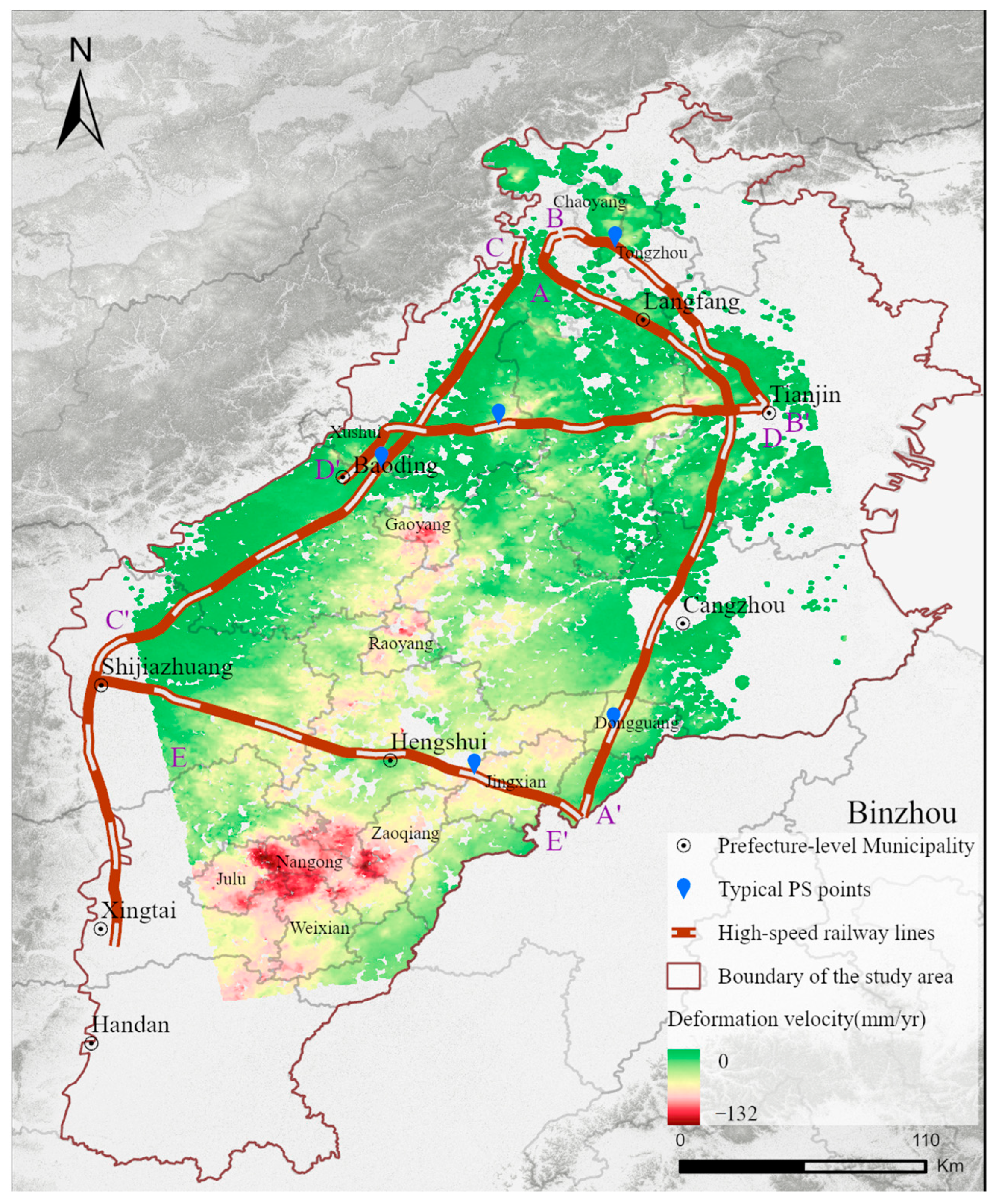
In the BTH Plain, there are various land subsidence funnels with an interregional continuous distribution between 2016 and 2020, as shown in Figure 3. The BTH plain’s center region had the most subsidence funnels, and these were distributed along a north–south strip. The main serious land subsidence was in Chaoyang–Tongzhou in Beijing, Wuqing in Tianjin, Bazhou in Langfang, Baoding, Hengshui, Xingtai, and Cangzhou. The maximum subsidence rates in the above areas are 64 mm/year, 94 mm/year, 70 mm/year, 119 mm/year, 130 mm/year, 132 mm/year, and 92 mm/year, respectively. The highest land subsidence rate in the radar data coverage area was 132 mm/year between January 2016 and September 2020.
Figure 3 shows, the distribution of high-speed railways, while Figure 4 shows the characteristics of land subsidence along the high-speed railways, showcasing those that travel through or are adjacent to the land subsidence area. The subsidence rates along the Beijing–Shanghai, Beijing–Tianjin, Beijing–Guangzhou, Tianjin–Baoding, and Shijiazhuang–Jinan high-speed railways range from 0–56 mm/year, 0–28 mm/year, 0–23 mm/year, 0–82 mm/year, and 2–77 mm/year, respectively. Figure 4d,e show that the land subsidence along the Tianjin–Baoding and Shijiazhuang–Jinan high-speed railways is relatively serious. The land subsidence regions of Wuqing, Langfang, and Xiongxian are traversed by the Tianjin–Baoding high-speed railway. Figure 4d shows that the maximum rate of land subsidence along the high-speed railway, which occurred 98 km from the starting point, reached 82 mm/year. Meanwhile, Figure 4e revealed that the amount of subsidence along the Shijiazhuang–Jinan high-speed railway is considerable, with 67% of the whole length of the high-speed railway having a subsidence rate over 30 mm/year. The railway spanned the subsidence area of Jing County, Hebei Province, of which the maximum subsidence rate was 77 mm/year and occurred 136 km away from the beginning site. As shown in Figure 3 and Figure 4a–c, the Beijing–Shanghai, Beijing–Tianjin and Beijing–Guangzhou high-speed railways are close to the subsidence areas of Dongguang County–Jingxian County, Chaoyang District–Tongzhou District, and Xushui County, and the overall subsidence is relatively slow. The largest subsidence rates, which were situated 250 km, 21 km, and 103 km from the starting point, were 55 mm/year, 28 mm/year, and 23 mm/year, respectively.
According to the cumulative subsidence and time series land subsidence data, the evolution characteristics of land subsidence along these lines were further analyzed from the perspective of time. We selected PS points with the maximum deformation rate along the line as typical points to analyze the cumulative subsidence and time series land subsidence (Figure 5). The position of the points is shown in Figure 3. As shown by the cumulative subsidence curve, from 2016 to 2020, land subsidence continued to occur at each typical point. Figure 5a–e show that the maximum cumulative subsidence of the Beijing–Shanghai, Tianjin–Baoding, and Shijiazhuang–Jinan high-speed railways reached 326 mm, 384 mm, and 350 mm, respectively. We further analyzed the changing characteristics of the land subsidence at typical points. The fluctuation degree of the curve in Figure 5 represents the uneven degree of the land subsidence time series change. Figure 5 shows that the subsidence of each typical point fluctuated from 2016 to 2020. The uneven evolution of the subsidence of typical points on the Beijing–Guangzhou high-speed railway is slightly weak, and the amplitude of the subsidence fluctuation is basically within 5 mm. The amplitudes of subsidence fluctuations at typical points on the Beijing–Tianjin and Beijing–Shanghai high-speed railways are approximately 10 mm. The uneven evolution degree of the time sequence subsidence of typical points on the Tianjin-Baoding high-speed railway and the Shijiazhuang–Jinan high-speed railway is the strongest, with maximum amplitudes reaching 16 mm and 12 mm, respectively. The time periods are from July to August 2016 and July to August 2018. In general, the spatial–temporal evolution of regional land subsidence certainly affects high-speed railways. Therefore, attention must be paid to the monitoring of land subsidence along high-speed railway lines.

4.2. Validation of Time-Series Results

To verify the accuracy of the land subsidence monitoring results obtained using the PS-InSAR technique, we selected seven leveling benchmarks in the study area from October 2016 to October 2017. Their positions are shown in Figure 1. We established buffers with a radius of 500 m around the leveling benchmark, and the subsidence of PS points was extracted within the buffer areas. We calculated the average subsidence of these PS points from October 2016 to 2017 and compared them with the leveling benchmark values. The results are shown in Table 2. We find that the maximum deviation between the results obtained by PS-InSAR monitoring and the leveling values is 11 mm, the minimum deviation is 0 mm, and the average deviation is 5 mm. The comparison shows that the monitoring results of PS-InSAR are accurate and can support this study.

5. Discussion

5.1. Land Subsidence Forecasting along High-Speed Railways Based on the EMD-GBDT Model

Land subsidence is characterized by nonlinear evolution, as shown in Figure 5, and the evolution of land subsidence is complex. To accurately forecast the land subsidence along the high-speed railway lines, the time series were broken down and the complexity of the original data was reduced using the EMD method. To improve the forecasting accuracy, we used a GBDT model for the decomposed IMF components and trend component.
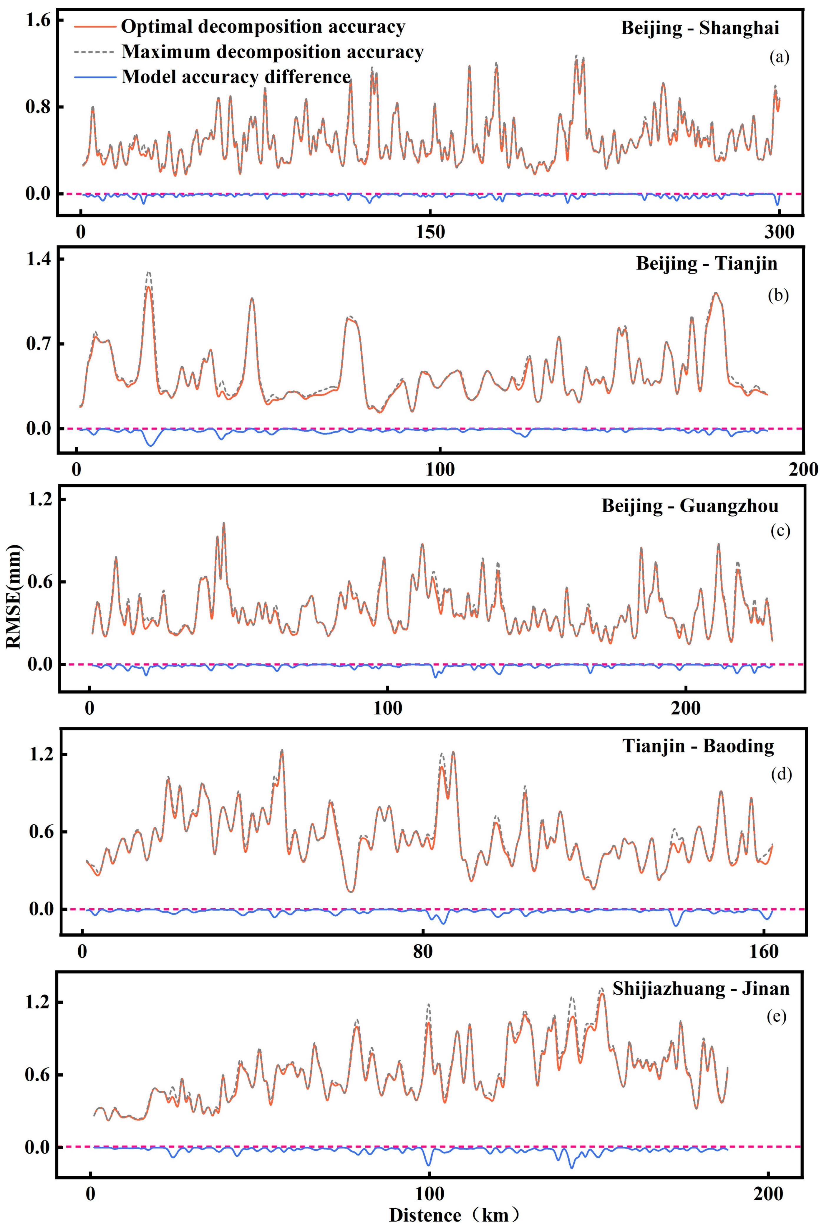
We extracted a PS point from each high-speed railway line as an example point for EMD. The subsidence values of these points were decomposed using the EMD method introduced in Section 3.2.1, and all IMF components and trend components are presented in Figure 6. As shown in Figure 6a–e, there were four IMF components of the Beijing–Tianjin and Beijing–Shanghai high-speed railways; the Beijing–Guangzhou, Tianjin–Baoding, and Shijiazhuang–Jinan high-speed railways had three. With the decomposition of the EMD method, the fluctuations in the original time series weakened. However, due to the different evolution characteristics of the sample points along the high-speed railways, the numbers of IMF components obtained from the EMD method were different. To ensure that the forecasting result of each sample point was the optimal value, each point was iteratively decomposed, and the IMF component obtained via the decomposition was modeled separately. We compared the error values forecasted by the GBDT models under different numbers of IMF components at sample points and selected the number of IMF components with the optimal error and the forecasting results at this time as the final forecasting results. The RMSE comparison of models between the optimal decomposition and the maximum decomposition for each high-speed railway is shown in Figure 7a–e. While constructing the EMD-GBDT and GBDT models, we mainly considered the selection of parameters used in the base learners and tree branches. We optimized and adjusted each of the model’s parameters based on the grid search approach to determine the optimal parameters, as shown in Table 3.
To contrast and verify the EMD-GBDT model’s correctness, we used the GBDT and ARIMA models. The results of the accuracy evaluation indexes of the three models are shown in Table 4, and the model forecasting results are shown in Figure 8a–e. Table 4 shows that the RMSE and MAE of the optimized EMD-GBDT model are the minimum, which indicates that our model has the best forecasting results for land subsidence in time series. The results also further demonstrated that the final forecasting effect and accuracy can be improved by reconstructing the forecasting values of IMF components and trend components in relation to the complex nonlinear characteristics of land subsidence in time series.

5.2. Analysis of Slope Changes along High-Speed Railways

Slope changes along a high-speed railway can minimize the impact of land subsidence on its safe operation [40]. Figure 8 demonstrates the continued, slow subsidence occurring along the high-speed railways. We calculated the slope changes using Formula (5) with the forecasted subsidence along each high-speed railway line and evaluated the stability of high-speed railway operation. The results were shown in Table 5. The formula used to calculate the slope is as follows [41]:
S = Δ h L
Δ h represents the land subsidence difference (m) of the upper two points along the high-speed railway and L represents the distance (m) between the two points. The results show that from January 2016 to September 2021, the impact of the differential evolution of land subsidence on the slope change along each high-speed railway was within the engineering technical standard (2‰). Most of the slope changes along high-speed railways are within 0.02‰. The influence of land subsidence along the Tianjin–Baoding high-speed railway on the slope changes range from 0.15‰ to 0.1‰, and the length of the high-speed railway within the range is 3.13 km.
In summary, these findings reveal a gradually growing tendency in the land subsidence along the typical high-speed rails in the BTH. High-speed railway slope variations are impacted by land subsidence, which has a direct impact on the stability of high-speed railway operations. Therefore, it is crucial to pay close attention to how the land subsidence along the high-speed train is developing.

6. Conclusions

Long-term groundwater overexploitation causes visible land subsidence in the BTH region [3,4,5]. Concurrently, the development of transportation integration causes high-speed railway networks to expand rapidly in the BTH region. In this study, based on the results of land subsidence from 2016 to 2020 in typical areas of the BTH region obtained by the PS-InSAR technique, we used the EMD-GBDT model to forecast the land subsidence along typical high-speed railways in 2021. Then, we analyzed the stability of high-speed railway operations. The conclusions are as follows:
  • From 2016 to 2020, the land subsidence mainly occurred in the middle BTH Plain, with a north–south zonal distribution. In numerous instances, multiple land subsidence funnels in the BTH Plain were connected into one. The maximum land subsidence rate reached 132 mm/year.
  • The subsidence along the Tianjin–Baoding and Shijiazhuang–Jinan high-speed railways was significant in the BTH region. The Tianjin–Baoding high-speed railway passed through the land subsidence areas of Wuqing, Langfang, and Xiongxian. The maximum subsidence rate along the Tianjin–Baoding high-speed railway reached about 82 mm/year.
  • The EMD-GBDT model can improve the forecasting accuracy of land subsidence to some degree. As of September 2021, the land subsidence has influenced slope changes along the high-speed railways, but it does not exceed the permitted technical standards.
Although this forecasting model has improved the accuracy of the forecast results, it also has some shortcomings. It did not consider the effect of different signal decomposition methods on the accuracy of the model. We will consider this issue in future studies.

Author Contributions

L.W. designed the experiments, implemented the algorithm, analyzed the results, and wrote the paper. C.Z. made important suggestions for writing the paper. H.G. and B.C. provided crucial guidance. X.X. helped organize the data. All authors have read and agreed to the published version of the manuscript.

Funding

This work was supported by National Natural Science Foundation of China (42201081, 41930109, 42371081, 42371089), Beijing Outstanding Young Scientist Program (BJJWZYJH01201910028032), R&D Program of Beijing Municipal Education Commission (KM 202210028010), Beijing Youth Top Talent Project, and National “Double-Class” Construction of University Projects.

Data Availability Statement

The SAR data can be downloaded from the following URL. ((https://scihub.copernicus.eu/ accessed on 22 June 2022). Other data can be accessed through the Data Sharing Infrastructure of the Earth System Science repository (https://doi.org/10.7910/DVN/Y44Y1G, accessed on 18 September 2023).

Acknowledgments

Thanks to the European Space Agency for the open-source Sentinel series data. Thanks to the reviewers and editors for their suggestions on this article.

Conflicts of Interest

The authors declare no conflict of interest.

References

  1. Gong, H.L.; Li, X.J.; Pan, Y.; Zhu, L.; Zhang, Y.Q.; Chen, M.; Chen, B.B.; Ke, Y.H.; Wang, Y.B.; Gao, M.L.; et al. Groundwater depletion and land subsidence of the Beijing-Tianjin-Hebei area. Bull. Natl. Nat. Sci. Found. China 2017, 1, 72–77. [Google Scholar] [CrossRef]
  2. Guo, H.; Zhang, Z.; Cheng, G.; Li, W.; Li, T.; Jiao, J.J. Groundwater-derived land subsidence in the North China Plain. Environ. Earth Sci. 2015, 2, 1415–1427. [Google Scholar] [CrossRef]
  3. Zhang, L.; Ge, D.Q.; Guo, X.F.; Wang, Y.; Li, M. Land subsidence in Cangzhou over the last decade based on interferometric time series analysis. Shanghai Land Resour. 2014, 35, 72–75+80. [Google Scholar] [CrossRef]
  4. Zhou, Y.; Luo, Y.; Guo, G.X.; Luo, Y.; Lei, K.; Wang, R. A study of the characteristics of land subsidence and the main control factors in the alluvial plain: A case study of Beijing plain. Geol. Bull. China 2016, 35, 2100–2110. [Google Scholar]
  5. Zhang, J.J.; Niu, W.M.; Lv, X.W.; Liu, Y.J.; Li, Z.N. Characteristics of land subsidence in an area of long-term groundwater mining in Tianjin. Shanghai Land Resour. 2019, 40, 77–80, 85. [Google Scholar] [CrossRef]
  6. Cui, W.J.; Lei, K.C. Some Ideas on Land Subsidence Working from the view of Coordinated Development in Beijing-Tianjin-Hebei Regions. Urban Geogr. 2018, 2, 25–30. [Google Scholar] [CrossRef]
  7. Cao, Q.; Chen, B.B.; Gong, H.L.; Zhou, C.F.; Luo, Y.; Gao, M.L.; Wang, X.; Shi, M.; Zhao, X.X.; Zuo, J.J. Monitoring of land subsidence in Beijing-Tianjin-Hebei Urban by combination of SBAS and IPTA. J. Nanjing Univ. Nat. Sci. 2019, 3, 381–391. [Google Scholar] [CrossRef]
  8. Gong, H.; Pan, Y.; Zheng, L.; Li, X.; Zhu, L.; Zhang, C.; Huang, Z.; Li, Z.; Wang, H.; Zhou, C. Long-term groundwater storage changes and land subsidence development in the North China Plain (1971–2015). Hydrogeol. J. 2018, 5, 1417–1427. [Google Scholar] [CrossRef]
  9. Berardino, P.; Fornaro, G.; Lanari, R.; Sansosti, E. A new algorithm for surface deformation monitoring based on small baseline differential SAR interferograms. IEEE Trans. Geosci. Electron. 2002, 11, 2375–2383. [Google Scholar] [CrossRef]
  10. Galloway, D.L.; Hudnut, K.W.; Ingebritsen, S.E.; Phillips, S.P.; Peltzer, G.; Rogez, F.; Rosen, P.A. Detection of aquifer system compaction and land subsidence using interferometric synthetic aperture radar, Antelope Valley, Mojave Desert, California. Water Resour. Res. 1998, 10, 2573–2585. [Google Scholar] [CrossRef]
  11. Hooper, A. A multi-temporal InSAR method incorporating both persistent scatterer and small baseline approaches. Geophys. Res. Lett. 2008, 35, 1–5. [Google Scholar] [CrossRef]
  12. Gao, M.; Gong, H.; Chen, B.; Zhou, C.; Chen, W.; Liang, Y.; Shi, M.; Si, Y. InSAR time-series investigation of long-term ground displacement at Beijing Capital International Airport. Tectonophysics 2016, 691, 271–281. [Google Scholar] [CrossRef]
  13. Ferretti, A.; Prati, C.; Rocca, F. Nonlinear subsidence rate estimation using permanent scatterers in differential SAR interferometry. IEEE Trans. Geosci. Remote Sens. 2000, 5, 2202–2212. [Google Scholar] [CrossRef]
  14. Wang, Y.; Bai, Z.; Zhang, Y.; Qin, Y.; Lin, Y.; Li, Y.; Shen, W. Using TerraSAR X-band and Sentinel-1 C-band SAR interferometry for deformation along Beijing-Tianjin Intercity Railway analysis. IEEE J-STARS 2021, 14, 4832–4841. [Google Scholar] [CrossRef]
  15. Malik, K.; Kumar, D.; Perissin, D.; Pradhan, B. Estimation of ground subsidence of New Delhi, India using PS-InSAR technique and Multi-sensor Radar data. Adv. Space Res. 2022, 69, 1863–1882. [Google Scholar] [CrossRef]
  16. Lu, Z.Z.; Chen, B.B.; Gong, H.L.; Zhou, C.F.; Shi, M.; Cao, J. Evolution Characteristics of Land Subsidence in Beijing Section of Beijing-Tianjin Intercity Railway before and after the South-to-North Water Diversion Project. Geomat. Inf. Sci. Wuhan Univ. 2023, 48, 1–19. [Google Scholar] [CrossRef]
  17. Ye, Y.; Yan, C.; Luo, X.; Zhang, R.; Yuan, G. Analysis of ground subsidence along Zhengzhou metro based on time series InSAR. Natl. Remote Sens. Bull. 2022, 26, 1342–1353. [Google Scholar] [CrossRef]
  18. Ye, S.J.; Xue, Y.Q.; Zhang, Y.; Li, Q.F.; Wang, H.M. Study on the deformation characteristics of soil layers in regional land subsidence model of Shanghai. Chin. J. Geotech. 2005, 27, 140–147. [Google Scholar] [CrossRef]
  19. Luo, Z.J.; Huang, X.R. Three-dimensional full coupling numerical simulation of groundwater exploitation and control of land-subsidence in region. J. Hydrodynam. A 2009, 5, 566–574. [Google Scholar]
  20. Zhu, L.; Franceschini, A.; Gong, H.; Ferronato, M.; Dai, Z.; Ke, Y.; Pan, Y.; Li, X.; Wang, R.; Teatini, P. The 3-D Facies and Geomechanical Modeling of Land Subsidence in the Chaobai Plain, Beijing. Water Resour. Res. 2020, 56, e2019WR027026. [Google Scholar] [CrossRef]
  21. Tomás, R.; Herrera, G.; Delgado, J.; Lopez-Sanchez, J.; Mallorquí, J.; Mulas, J. A ground subsidence study based on DInSAR data: Calibration of soil parameters and subsidence prediction in Murcia City (Spain). Eng. Geol. 2010, 111, 19–30. [Google Scholar] [CrossRef]
  22. Yue, Z.H.; Shen, T.; Mao, X.; Ma, W.J. Study on prediction method of land subsidence based on recurrent neural network. Sci. Surv. Mapp. 2020, 45, 145–152. [Google Scholar] [CrossRef]
  23. Edalat, A.; Khodaparast, M.; Rajabi, A.M. Scenarios to control land subsidence using numerical modeling of groundwater exploitation: Aliabad plain (in Iran) as a case study. Environ. Earth Sci. 2020, 21, 1–12. [Google Scholar] [CrossRef]
  24. Fan, S.S.; Guo, H.P.; Zhu, J.Y.; Li, W.P. Application of linear regression model for land subsidence prediction in Beijing plain. Chin. J. Geol. Hazard Control 2013, 24, 70–74. [Google Scholar] [CrossRef]
  25. Deng, Z.; Ke, Y.H.; Gong, H.L.; Li, X.; Li, Z. Land subsidence prediction in Beijing based on PS-InSAR technique and improved Grey-Markov model. GIsci Remote Sens. 2017, 6, 797–818. [Google Scholar] [CrossRef]
  26. Zhao, Z.H.; Hu, X.P.; Sun, H.M.; Zhang, S.X.; Zhang, B. Application of BP Neural Network in Prediction of Ground Settlement in Urban Shield Tunneling. Subgrade Eng. 2020, 4, 170–175. [Google Scholar] [CrossRef]
  27. Wang, J.M.; Zhang, J. Deformation Intelligent Prediction Model Based on Gaussian Process Regression and Application. Geomat. Inf. Sci. Wuhan Univ. 2018, 43, 248–254. [Google Scholar] [CrossRef]
  28. Arabameri, A.; Saha, S.; Roy, J.; Tiefenbacher, J.P.; Cerda, A.; Biggs, T.; Pradhan, B.; Ngo, P.T.T.; Collins, A.L. A novel ensemble computational intelligence approach for the spatial prediction of land subsidence susceptibility. Sci. Total Environ. 2020, 726, 138595. [Google Scholar] [CrossRef]
  29. Guo, H.P.; Li, W.P.; Wang, L.Y.; Chen, Y.; Zang, X.; Wang, Y.; Zhu, J.; Bian, Y. Present situation and research prospects of the land subsidence driven by groundwater levels in the North China Plain. Hydrogeol. Eng. Geol. 2021, 3, 162–171. [Google Scholar] [CrossRef]
  30. Wegmüller, U.; Werner, C.; Strozzi, T.; Wiesmann, A. Multi-temporal interferometric point target analysis. In Proceedings of the Analysis of Multi-Temporal Remote Sensing Images-The Second International Workshop, Ispra, Italy, 1 August 2004. [Google Scholar] [CrossRef]
  31. Perissin, D.; Wang, Z.Y.; Wang, T. The SARPROZ InSAR tool for urban subsidence/manmade structure stability monitoring in China. In Proceedings of the 34th International Symposium on Remote Sensing of Environment, Sydney, Australia, 10–15 April 2011. [Google Scholar]
  32. Huang, N.E.; Zhang, S.; Long, S.R.; Wu, M.C.; Shih, H.H.; Zheng, Q.; Yen, N.C.; Tung, C.C.; Liu, H.H. The empirical mode decomposition and the Hilbert spectrum for nonlinear and non-stationary time series analysis. Proc. R. Soc. Lond. 1998, 454, 903–995. [Google Scholar] [CrossRef]
  33. Beckheinrich, J.; Hirrle, A.; Schon, S.; Beyerle, G.; Semmling, M.; Wickert, J. Water level monitoring of the Mekong Delta using GNSS reflectometry technique. In Proceedings of the 2014 IEEE Geoscience and Remote Sensing Symposium, Quebec City, QC, Canada, 13–18 July 2014. [Google Scholar]
  34. Rilling, G.; Flandrin, P.; Goncalves, P. On empirical mode decomposition and its algorithms. In Proceedings of the IEEE-EURASIP Workshop on Nonlinear Signal and Image Processing NSIP-03, Grado, Italy, 8–11 June 2003. [Google Scholar]
  35. Friedman, J.H. Greedy Function Approximation: A Gradient Boosting Machine. Ann. Stat. 2001, 5, 1189–1232. [Google Scholar] [CrossRef]
  36. Wu, W.; Wang, J.; Huang, Y.; Zhao, H.; Wang, X. A novel way to determine transient heat flux based on GBDT machine learning algorithm. Int. J. Heat Mass Transfer. 2021, 179, 121746. [Google Scholar] [CrossRef]
  37. Zhang, H.Y.; Wu, W.S.; Wu, H. TOC prediction using a gradient boosting decision tree method: A case study of shale reservoirs in Qinshui Basin. Geoenergy Sci. Eng. 2023, 221, 111271. [Google Scholar] [CrossRef]
  38. Zhou, J.; Huang, S.; Tao, M.; Khandelwal, M.; Dai, Y.; Zhao, M. Stability prediction of underground entry-type excavations based on particle swarm optimization and gradient boosting decision tree. Undergr. Space 2023, 9, 234–249. [Google Scholar] [CrossRef]
  39. Zhang, X.H.; Ren, X.D.; Wu, F.; Lu, Q. Short-term Prediction of Ionospheric TEC Based on ARIMA Model. J. Geod. Geoinf. Sci. 2019, 2, 9–16. [Google Scholar] [CrossRef]
  40. Li, G.H.; Xu, Z.L.; Sun, S.L.; Jing, Z.D. The Influence of Surface Subsidence on Construction of High-speed Railway in North China Plain and Its Countermeasures. J. Railw. 2007, 8, 7–12. [Google Scholar]
  41. Xie, H.L.; Xia, Y.B.; Meng, Q.H.; Zhao, C.R.; Ma, Z. Study on land subsidence assessment in evaluation of carrying capacity of geological environment. Geol. Surv. Res. 2019, 2, 104–108. [Google Scholar] [CrossRef]
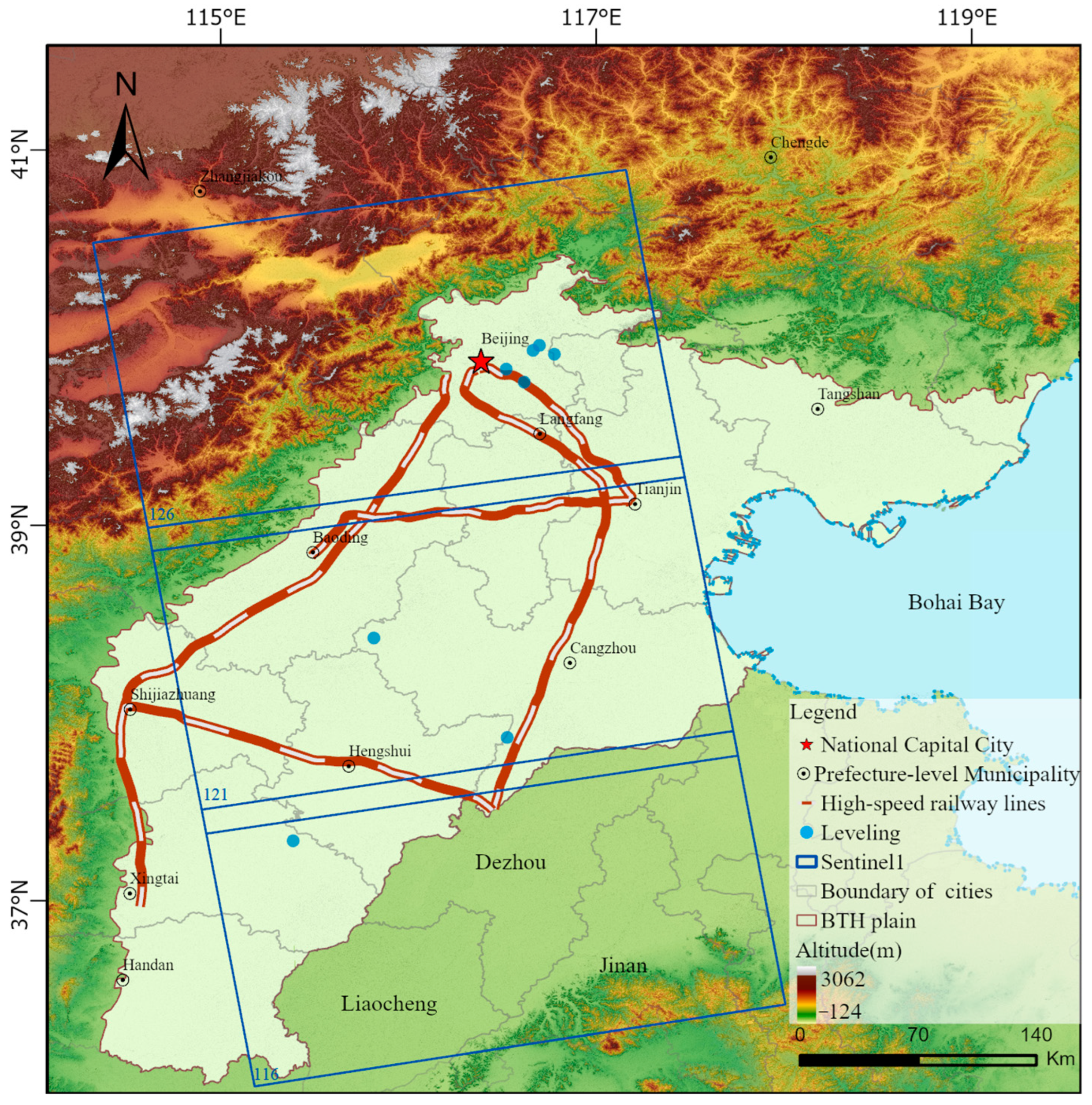
Figure 1. Overview of the study area (the blue borders present the spatial coverage of Sentinel-1A, and the light sky-blue dots represent the leveling benchmarks for trialing land subsidence results).
Remotesensing 15 04606 g001
Figure 2. Flow chart of EMD-GBDT model.
Remotesensing 15 04606 g002
Figure 3. Distribution of average subsidence rate in BTH typical areas from 2016 to 2020.
Remotesensing 15 04606 g003
Figure 4. Land subsidence rate along the high-speed railways in the typical BTH area. Land subsidence rate along the Beijing–Shanghai (a), Beijing–Tianjin (b), Beijing–Guangzhou (c), Tianjin–Baoding (d) and Shijiazhuang–Jinan (e) high-speed railways from 2016 to 2020.
Remotesensing 15 04606 g004
Figure 5. Panels (ae) show the cumulative and time series land subsidence of typical PS points on Beijing–Shanghai (a), Beijing–Tianjin (b), Beijing–Guangzhou (c), Tianjin–Baoding (d), and Shijiazhuang–Jinan (e) high-speed railways, respectively. The red and the light sky-blue solid lines represent cumulative and time-series land subsidence, respectively.
Remotesensing 15 04606 g005
Figure 6. EMD decomposition results of original time series subsidence of typical PS points on Beijing–Shanghai (a), Beijing–Tianjin (b), Beijing–Guangzhou (c), Tianjin–Baoding (d) and Shijiazhuang–Jinan (e) high speed railways.
Remotesensing 15 04606 g006
Figure 7. Comparison of model RMSE between the optimal IMF decomposition and the maximum decomposition for Beijing–Shanghai (a), Beijing–Tianjin (b), Beijing–Guangzhou (c), Tianjin–Baoding (d) and Shijiazhuang–Jinan (e) high-speed railways. The red and the blue solid lines represent optimal decomposition accuracy and model accuracy differences, respectively. The gray dotted line shows maximum decomposition accuracy.
Remotesensing 15 04606 g007
Figure 8. The forecasting result of subsidence along Beijing–Shanghai (a), Beijing–Tianjin (b), Beijing–Guangzhou (c), Tianjin–Baoding (d) and Shijiazhuang–Jinan (e) high-speed railways based on EMD-GBDT (purple line), GBDT (cyan line), and ARIMA (red line) models (the time series of the original value range from January 2016 to September 2020 and EMD-GBDT, signal GBDT, and ARIMA models range from January 2016 to September 2021).
Remotesensing 15 04606 g008
Table 1. S1A Radar Image Information.
SAR SensorSentinel-1A (S1A)
Orbit directionAscending
Spatial resolution(m)5 m × 20 m
BandC-band
PolarizationVV
Beam ModeInterferometric Wide swath (IW)
Repeat observation period(day)12
Number of images204
Date range14 January 2016–1 September 2020
Table 2. Comparison between PS-InSAR and leveling monitoring results.
Benchmarks NumberPS-InSAR (mm)Leveling Measurement (mm)Difference (mm)
1220
26159
3594
4263610
5121
688891
7799011
Table 3. Parameter list of EMD-GBDT and GBDT model.
ModelParametersValueParametersValue
EMD-GBDT/GBDTlossMSEmax_depth2
learning_Rate0.13min_samples_split6
n_estimators50min_samples_leaf0.04
Random Seed10subsample0.85
Table 4. Comparison of accuracy indexes of EMD-GBDT and GBDT, ARIMA models.
ModelEMD-GBDTGBDTARIMA
Evaluating indicatorRMSEMAERMSEMAERMSEMAE
Beijing–Shanghai0.470.290.490.301.160.90
Beijing–Tianjin0.430.270.450.280.960.73
Beijing–Guangzhou0.380.230.390.240.870.68
Tianjin–Baoding0.540.320.560.331.230.95
Shijiazhuang–Jinan0.560.380.590.41.431.15
Note: The bold represents the smallest error corresponding index of the model and the units of RMSE and MAE values are in millimeters.
Table 5. Impact of land subsidence differential evolution on slope change of typical Beijing–Tianjin–Hebei high-speed railways from 2016 to 2021.
Slope Variation Range (‰)0–0.020.02–0.040.04–0.060.06–0.080.08–0.10.1–0.15
Beijing-Shanghai83.2813.712.340.67--
Beijing-Guangzhou93.655.820.53---
Beijing-Tianjin93.425.260.880.44--
Tianjin-Baoding60.6319.379.372.553.13
Shijiazhuang-Jinan69.5223.535.351.070.53-
Note: The symbol “-” indicates that there are no data in the range.
Disclaimer/Publisher’s Note: The statements, opinions and data contained in all publications are solely those of the individual author(s) and contributor(s) and not of MDPI and/or the editor(s). MDPI and/or the editor(s) disclaim responsibility for any injury to people or property resulting from any ideas, methods, instructions or products referred to in the content.