Article

Enhancing Land Cover Mapping and Monitoring: An Interactive and Explainable Machine Learning Approach Using Google Earth Engine

1
Interdisciplinary Science Cooperative, University of New Mexico, Albuquerque, NM 87131, USA
2
Department of Geography and Environmental Studies, University of New Mexico, Albuquerque, NM 87131, USA
3
Center for the Advancement of Spatial Informatics Research and Education (ASPIRE), University of New Mexico, Albuquerque, NM 87131, USA
4
Department of Computer Science, University of New Mexico, Albuquerque, NM 87106, USA
5
Department of Geography & Sustainability, University of Tennessee, Knoxville, TN 37996, USA
*
Author to whom correspondence should be addressed.
Remote Sens. 2023, 15(18), 4585; https://doi.org/10.3390/rs15184585
Submission received: 8 August 2023 / Revised: 9 September 2023 / Accepted: 14 September 2023 / Published: 18 September 2023
(This article belongs to the Special Issue Explainable Artificial Intelligence (XAI) in Remote Sensing Big Data)

Abstract

:
Artificial intelligence (AI) and machine learning (ML) have been applied to solve various remote sensing problems. To fully leverage the power of AI and ML to tackle impactful remote sensing problems, it is essential to enable researchers and practitioners to understand how AI and ML models actually work and thus to improve the model performance strategically. Accurate and timely land cover maps are essential components for informed land management decision making. To address the ever-increasing need for high spatial and temporal resolution maps, this paper developed an interactive and open-source online tool, in Python, to help interpret and improve the ML models used for land cover mapping with Google Earth Engine (GEE). The tool integrates the workflow of both land cover classification and land cover change dynamics, which requires the generation of a time series of land cover maps. Three feature importance metrics are reported, including impurity-based, permutation-based, and SHAP (Shapley additive explanations) value-based feature importance. Two case studies are presented to showcase the tool’s capability and ease of use, enabling a globally accessible and free convergent application of remote sensing technologies. This tool may inspire researchers to facilitate explainable AI (XAI)-empowered remote sensing applications with GEE.

1. Introduction and Motivation

Artificial intelligence (AI) has diffused into many areas of our private and professional lives and influences how we live and work. Moreover, it is increasingly being used in critical situations with potentially severe consequences for individual human beings, businesses, and society as a whole [1]. AI has also advanced various applications in many parts of the Earth’s system (land, ocean, and atmosphere) and beyond [2,3]. Remote sensing (RS) provides science-quality big Earth observation data for understanding the Earth system and policy development [4]. The rapid increase in geospatial big data, among which RS big data comprises a big portion, poses significant challenges to conventional geographic information systems (GIS) as well as RS approaches and platforms [5]. AI, especially its branches of machine learning (ML) and deep learning (DL), have advanced many domains, including RS and even complex problems in Earth sciences and geosciences [2,3,6,7,8,9,10]. However, most of the AI applications in many domains still stay in the “black box” stage. We need AI/ML models to function as expected, to produce transparent results and explanations, and to be visible in how they work [11]. Domain researchers cannot really understand and explain why an ML/DL model works well or why it does not work well for a specific domain problem [11]. This motivates the emerging AI research topic explainable artificial intelligence (XAI) [12], the goal of which is to unbox how AI systems’ black-box choices are made [13,14,15]. More specifically, XAI enables humans to understand the models to effectively manage the benefits that AI systems provide while maintaining a high level of prediction accuracy; XAI helps scientists to gain insights about the decision strategy of AI/ML models, supports fine tuning and optimizing models, and helps gauge trust [3,11,16].
AI algorithms utilize mathematical models to learn the fundamental features from a dataset to make a prediction [15]. To understand how machine learning models work under the hood, feature selection plays an essential role [5,17]. As emphasized in [18], “... one obstacle to overcome is the lack of explainability in some parts of the scientific process. Future directions would be to develop methods to understand which features in an image that triggers a certain response and relate that to domain knowledge; is the response and features in accordance with theory within the field(s)?”. Different feature importance (also called variable importance) metrics have been developed to evaluate which set of features are important for increasing model prediction performance [19,20]. Most tree-based ML classifiers provide a built-in measure of feature importance based on the mean decrease in impurity (MDI). The computation of this impurity-based importance is fast as all needed values are already computed when training the classifier. As an alternative, permutation feature importance is defined as the decrease in a model score (accuracy) when a single feature value is randomly shuffled [20]. Permuting the values of the most important features will lead to the greatest decrease in the model’s accuracy score.
Both impurity-based importance and permutation feature importance are traditional metrics assessing feature contribution to the overall model performance. However, to explain how different features contribute to a specific prediction for a sample, one has to resort to local explanation-enabled XAI models. Shapley additive explanations (SHAP) feature importance is such an alternative, which is a state-of-the-art explainable framework initially proposed in [21]. While permutation feature importance is based on the decrease in model performance (accuracy), SHAP is based on the magnitude of feature attributions. It uses the Shapley values from the classic game theory to estimate how much each feature contributes to the prediction, i.e., each of the individual classes [22]. Because of its strong theoretical foundation and abundant visualization tools, the SHAP method has recently been applied to various natural hazard mapping studies. Iban and Bilgilioglu [23] utilized SHAP to examine factors affecting the avalanche susceptibility of ski resorts. It was found that higher elevations (>2000 m) and steeper slopes (>30 degrees) increase the likelihood of an avalanche while a higher maximum temperature decreases the likelihood of an avalanche. Pradhan et al. [24] found through SHAP plots that land use and various soil attributes significantly affected flood susceptibility. Dahal and Lombardo [25] studied landslide susceptibility in an earthquake-induced hazard scenario. The SHAP values plot showed that the mean clay content, slope per slope unit, and peak ground velocity dominate the probability of landslide occurrence. A web application was even built to demonstrate the XAI model results.
Google Earth Engine (GEE), which is a scalable, cloud-based geospatial retrieval and processing platform, provides free access to a multi-petabyte archive of geospatial datasets spanning over 40 years of historical and current Earth observation (EO) imagery [5,26,27]. The high-resolution mapping of global forest cover changes [28] and global surface water [29] are two influential applications of GEE. With the various built-in geoprocessing algorithms and the Earth Engine API, users can instantly access and efficiently process petabytes of geospatial data in parallel using Google’s vast computational resources. The GEE’s web-based (Javascript) code editor enables user-interactive algorithm development, rapid prototyping, and visualization of results. If AI is integrated with GEE, as emphasized in [5], it will advance many (geospatial) relevant domains. There has been a plethora of land cover mapping studies using GEE. To the best of our knowledge, however, most of these studies exploring XAI with GEE used only the built-in feature importance (MDI) of the random forest (RF) classifier. There are few studies that adopt permutation or SHAP feature importance to interpret the ML models used for land cover classification [22,30].
Accurate and timely land use land cover (LULC) maps are essential tools for informed land management decision making. With the increasing availability of RS data, the need for high spatial and temporal resolution land cover maps is ever-increasing. Furthermore, these maps need to be tailored to the area of interest and accommodate the inherent heterogeneity of the land surface, which would result in different categorical LULC classes across different geographical and ecological conditions. Nowadays, there is a growing trend towards open-source tools, which require limited technical skills to extract tailored information for a specific area of interest (AOI) [31,32,33]. In the context of land cover mapping with GEE, two such tools are available: REMAP [34] and O-LCMapping [35]. They were implemented primarily in JavaScript, and it is not very straightforward and intuitive for other researchers and practitioners to adapt them to solve their domain problems. Both tools [34,35] excluded feature importance analysis in their workflows. In addition, in the AI setting, Python is the primarily used language, and it has more open-source resources for Earth observation researchers to better apply AI to solve their domain problems using GEE and XAI. While the popular SHAP model has already been applied to various geohazards mapping studies [23,24,25], it has seldom been applied to multi-label land cover mapping studies [22,36].
In this paper, an interactive visual tool was developed by leveraging AI with GEE to demonstrate land cover classification and monitoring. The open-source tool was implemented using Python. It integrates the workflow of static land cover classification, which is a snapshot in time, with land change dynamics, which require the generation of a time series of land cover maps. More specifically, our interactive tool allows users to examine the impurity-based, permutation-based, and SHAP-value-based feature importances of the ML models, allowing users to determine the most important features for their applications. The following sections describe an overview of the implementation, the workflow for land cover mapping and monitoring, the feature importance metrics, and other post-processing visualization plots that can be generated after the classification workflow. Two case studies are presented to illustrate the tool’s functionality. The code and accompanying video tutorials are available to the public (see Data Availability Statement part for details).

2. Approach

2.1. Implementation Overview

The explainable machine learning tool developed in this work is a Jupyter notebook that can be run directly on Google Colaboratory (Google Colab), which requires no setup on local computers and runs entirely in a browser by remotely connecting with Google’s cloud servers. The core functionality of the notebook is built mainly upon two Python packages geemap [31] and ipywidgets [37]. geemap is a Python package for interactive mapping with GEE, which uses the Python API to make computational requests to the Earth Engine servers. Empowered by ipyleaflet [38] and ipywidgets, geemap allows users to interactively analyze and visualize the Earth Engine datasets with Jupyter notebooks. The scikit-learn [39] and shap [40] packages are also used to calculate the feature importance values. The Colab’s layout widgets are used to organize the classification results and feature importance plots into different display tabs. Figure 1 shows the land cover mapping user interface created by ipywidgets and the various Colab tabs displaying the results. It should be noted that while the display tabs may work only on Colab, the main functionalities of the land cover mapping workflow should work on other platforms running Jupyter notebooks.

2.2. Workflow for Land Cover Classification

The typical steps for performing a land cover classification consist of determining the study area, selecting the data source (satellite sensors/bands) and the range of dates to extract the composite image to be classified, preparing sufficient labeled data for supervised classification, selecting a classifier with default or custom parameters, classifying the image, and performing accuracy assessments and some post-processing visualizations. Figure 2 shows the workflow chart of the land cover mapping tool developed in this work.
Several options are provided for the user to define the region of interest (ROI): (1) the user draws a geometry (circle, rectangle, and polygon) directly on the map; (2) the user inputs a single point coordinate and buffer size; (3) the user inputs the bounding box coordinates of a rectangle; or (4) the user uploads a GeoJSON file for a predefined geometry.
Table 1 lists the satellite/band information and spectral indices that are currently supported by the land cover mapping tool. Note that the Landsat Collection 2 imagery is used, as all data acquired after 31 December 2021 are only available in this collection. For the Sentinel-2 imagery, the HARMONIZED collection is used, which removes the band-dependent offset added to reflectance bands in newer scenes. The present implementation also supports multi-source satellite data for land cover mapping, which is achieved by simply stacking bands from different satellites (e.g., Landsat 8 and Sentinel-2). Several spectral indices (NDVI, NDWI, and NBR) and topographic variables (elevation and slope) are additional features that may be used to classify the land cover. The Shuttle Radar Topography Mission (SRTM) V3 product provided by NASA JPL is used in this study to extract the elevation and slope. This dataset has undergone a void-filling process using open-access data [41]. Other indices and climatic variables (such as mean annual temperature and precipitation) can be added easily in the future. Given the region of interest, the date interval, and the predictor variables selected, a composite image is then generated by applying spatial and temporal reducers in GEE. All the image preprocessing operations such as cloud masking, scaling, and clipping were performed in GEE.
The generation of high-quality labeled data is a laborious effort. Normally, the collection of the labeled data is conducted well ahead of the classification task. Users have two options to provide the labeled data. The first option is to upload a CSV file, tabulating the longitude/latitude of sample locations and class labels. The predictor variables (i.e., feature values) at these locations are then extracted from the composite image to be classified. Users can either embed the land cover class names as the labels column in the CSV file or provide the class names separately. Custom colors can be specified for each of the classes.
The second option is to generate samples directly from known land cover products, such as ESA’s WorldCover [42,43], Esri’s Global Land Cover [44], and Google’s Dynamic World V1 [45]. All three global land use land cover (LULC) maps were derived from the Sentinel satellites at 10 m resolution. While the first two maps are a yearly composite available for several discrete years only, the Dynamic World is a near-real-time LULC product that includes class labels as well as class probability scores. A cross-comparison study found large inaccuracies and spatial/thematic biases in each product that vary across biomes, continents, and human settlement types [46]. To generate the labeled data, both random sampling and stratified sampling are supported. The class names and palettes are extracted from the predefined class table of the land cover product.
Two supervised classifiers are supported at the time: classification and regression tree (CART) and random forest (RF). The default classifier parameters can be altered if so desired. But the calculation of feature importances is only available for the RF classifier. The values of all the predictor variables are extracted from the composite image pixels intersecting the geometries (Point in GEE) of the labeled dataset, which are then split into a training and a testing dataset. The training dataset is used to train the classifier, while the testing dataset is used to evaluate the classifier accuracy. The trained classifier is then used to classify the image to generate a land cover map, which can be exported to other platforms for further processing.

2.3. Post-Processing Visualization Toolkit

During the various stages of land cover classification, several layers are added in sequence to the ipyleaflet basemap, including the sample data, the composite image to be classified, and the classified image with a customizable legend. For the sample data, the training dataset and the testing dataset are marked with different shapes. A labels histogram for all of the samples and a parallel coordinate plot for the testing samples are also generated. Parallel coordinate plot (PCP) is a common way of visualizing and analyzing high-dimensional datasets. The class palette for the different land cover types is consistent among the samples/classified image layers on the map, the labels histogram, the PCP, the SHAP values summary plot, and the zonal areas plot.
As an integral step of the land cover mapping workflow, it is critical to perform a classifier assessment. The scikit-learn package is used to output a classification report for both GEE and scikit-learn’s random forest classifiers. To do so, the same training and testing sample data for the GEE classifier are exported. The training data are used to train the scikit-learn classifier, which then makes predictions on the testing dataset. Included in the classification report are precision, recall, and F1-score for all of the land cover classes and an overall accuracy score. The confusion matrix for both classifiers is calculated and plotted with different normalization options for interactive display.
A number of methods are employed to calculate and explore the feature importance, including impurity-based importance, permutation importance, and SHAP-value-based feature importance. More details about these metrics are described in the following section. Note that the computed feature importance does not reflect the intrinsic predictive value of a feature by itself. It just describes how important this feature is for a particular machine learning model. The more accurate a model is, the more trustworthy these numbers are. Users also have the option to calculate the zonal areas occupied by different land cover classes in the classified image. A bar plot and tabulated data are provided to show these statistics.

2.4. Feature Importance

The impurity-based importance, permutation feature importance, and SHAP were introduced in Section 1. Below, a bit more in-depth introduction is provided. The first two feature importance metrics have been traditionally adopted to optimize the feature space in order to improve the model performance. Each feature is assigned an overall importance score. Impurity-based importance is derived from statistics on the training dataset only and may not reflect the actual predictive ability of the features that should generalize to the held-out testing dataset. Moreover, this metric tends to be biased towards numerical features and categorical features with high cardinality (i.e., features with many unique values). In GEE, the RF classifier smileRandomForest [47] returns the sum of the decrease in impurity over all trees in the forest as the feature importance. The higher the value, the more important the feature. In the scikit-learn [48] RF classifier, the importance of a feature is computed as the (normalized) total reduction in the impurity brought by that feature; the sum of all feature importance values is equal to 1. Permutation feature importance can be computationally expensive as the model score needs to be calculated many times with different permutations for all of the features. It can be calculated on both the training and testing datasets. While GEE supports only the impurity-based importance, scikit-learn has its own implementation of both the impurity-based and the permutation importance.
In contrast to the global feature importance metrics mentioned above, SHAP uses the Shapley values from the classic game theory to fairly assign each feature’s contribution. As summarized in [24], SHAP values are unique for each feature, class (LULC in this study), and sample. For every data point, positive/negative values indicate positive/negative contributions of each feature to every possible class. A larger mean absolute Shapley value (|SHAP|) across all data points indicates a feature’s overall greater importance. It is a more robust approach as opposed to the traditional metrics. It also considers the interactions between features. Thus, apart from providing a global explanation of the classifier, the SHAP model also gives local insight into how each feature contributes to the sample-wise attribution. The SHAP approach is model-agnostic and can be applied to explain the output of many ML models, ranging from tree ensemble models to deep learning models. The shap Python library [40] also provides many visualization tools to help to interpret the model predictions, including summary bar plot, beeswarm plot, waterfall plot, scatter plot, force plot, and dependence plot.

2.5. Land Cover Change

Apart from the land cover classification described in Section 2.2, which is a snapshot in time, the same workflow is also capable of dynamically classifying land covers over a certain interval (yearly, monthly, etc.). In other words, a time series of LULC maps can be generated. This paves the way for a more in-depth analysis of the spatial and temporal evolutions of land covers (e.g., wetland monitoring [49,50,51]) and other systems (e.g., the coastal ecosystem studied in [52]) that can be accommodated by the classification workflow.
This function of land cover monitoring is enabled when the temporal interval of compositing images is chosen to be ‘yearly’, ‘monthly’, or ‘daily’ (using this option sparingly). Compared to the snapshot classification, the workflow of dynamic classification differs only in the generation of composite images and the extraction of predictors’ values for the labeled samples. The satellite images are sorted by acquisition date, and those images whose dates fall into a specific year or month are reduced into a median composite image. If the labeled data have a ‘date’ property (see the fourth column in the example CSV in Figure 2), predictor variables are extracted from the satellite images captured on the same day as the sample collection date. Otherwise, predictor variables are extracted from the median composite for the entire date range. A single classifier is then trained and applied to classify all of the yearly or monthly composite images. Ideally, a labeled dataset should be provided for each composite image, and the trained classifier is then used to classify that specific image. The entire set of classified composite images can be exported as a GIF animation, and the classified maps for specific years can be displayed in an image grid. The time series of zonal areas for each land cover class can be generated as well.

3. Case Studies

Two case studies are presented to demonstrate the use of the developed land cover mapping and monitoring tool. The first case classified the land cover for a rectangular region in the San Francisco Bay area, USA (Section 3.1). The second case examined the land cover change for each year between 2000 and 2020, in a coastal region off Dubai, United Arab Emirates (Section 3.2). Both case studies have been implemented in Python. More specifically, the interactive tool was implemented on Google Colab by leveraging GEE via geemap [31] and ipywidgets.

3.1. Land Cover Classification around San Francisco Bay

Figure 3 shows three snapshots in the land cover classification process for a focal region around San Francisco Bay. The natural color (Figure 3a, red/green/blue) composite image was obtained from the Sentinel-2 Level-2A imagery for the entire year of 2021. The labeled data (Figure 3b) were generated by stratified sampling (100 samples for each class) of Esri’s global land cover product [44]. The spectral bands in Sentinel-2 (B2–B5, B8, B9, B11, and B12), two spectral indices (NDVI and NDWI), and two topographic variables (elevation and slope) from the NASA SRTM V3 product were selected as the predictor variables. An RF classifier was trained, and the composite image was classified as shown in Figure 3c. The RF model was chosen because, as reported in [5], it is the most robust and widely used ML model available on GEE for various Earth observation-based applications (e.g., wetland mapping and wildfire). The labels histogram, the parallel coordinate plot, the classifier metrics and the confusion matrix, and the zonal areas for each land cover are available for review as well.
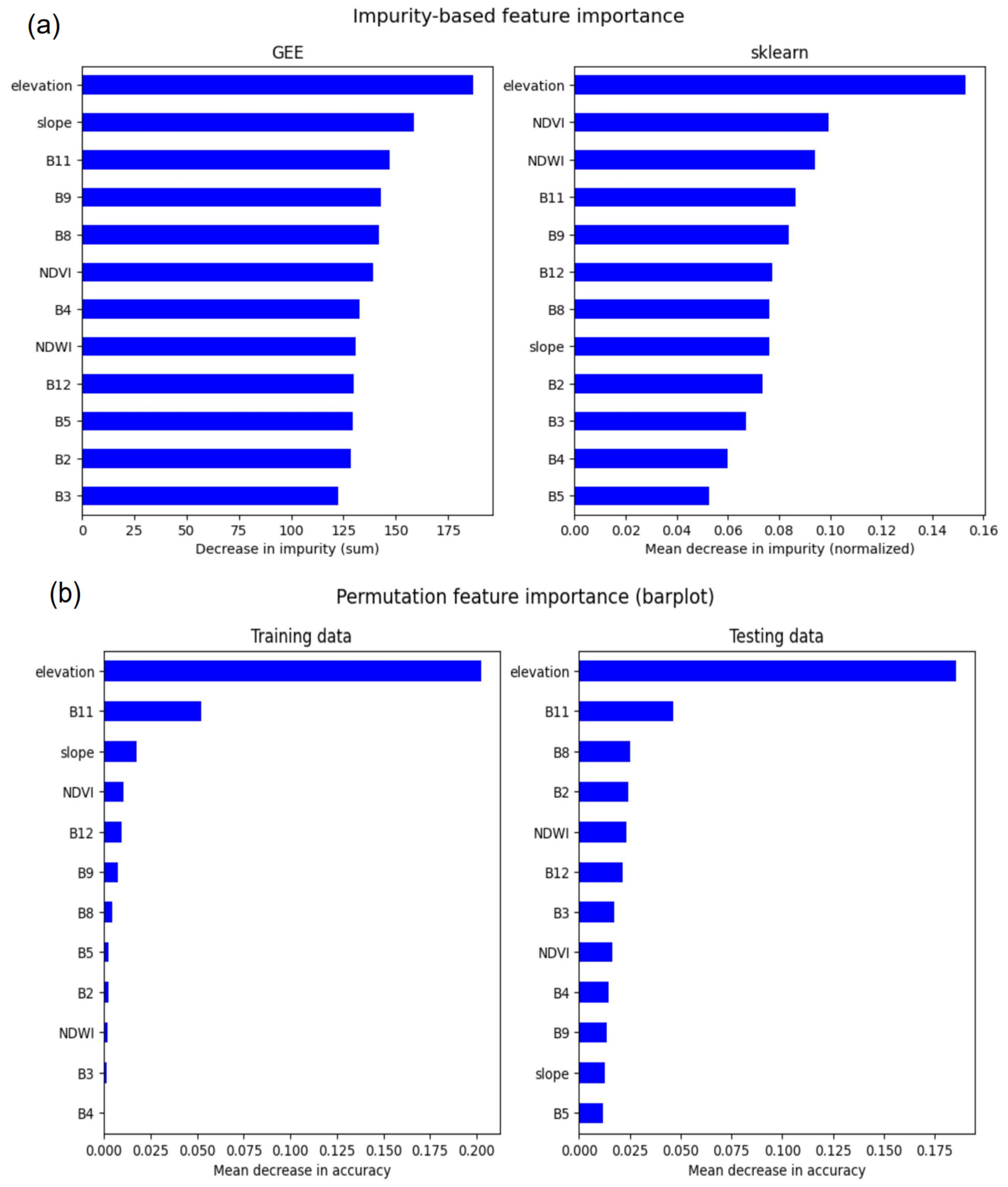
Figure 4 shows the feature importance computed by both the GEE and scikit-learn’s RF classifier. The impurity-based feature importance (Figure 4a) is only available for the training dataset. Note the different scales in the feature importance calculated by both classifiers. There are some differences in the order of the features with descending importance. Figure 4b shows the permutation feature importance calculated by using sk-learn’s RF classifier. Both the training and testing data were used to calculate the feature importance. Even though the same classifier was applied to the training and testing data, the feature sequences differ slightly. The two most important features (‘elevation’ and ‘B11’) were the same. Compared to the impurity-based feature importance (Figure 4a, right panel), this permutation importance roughly identifies the features of the most (‘elevation’ and ‘B11’) and least (‘B3’ and ‘B4’) importance.
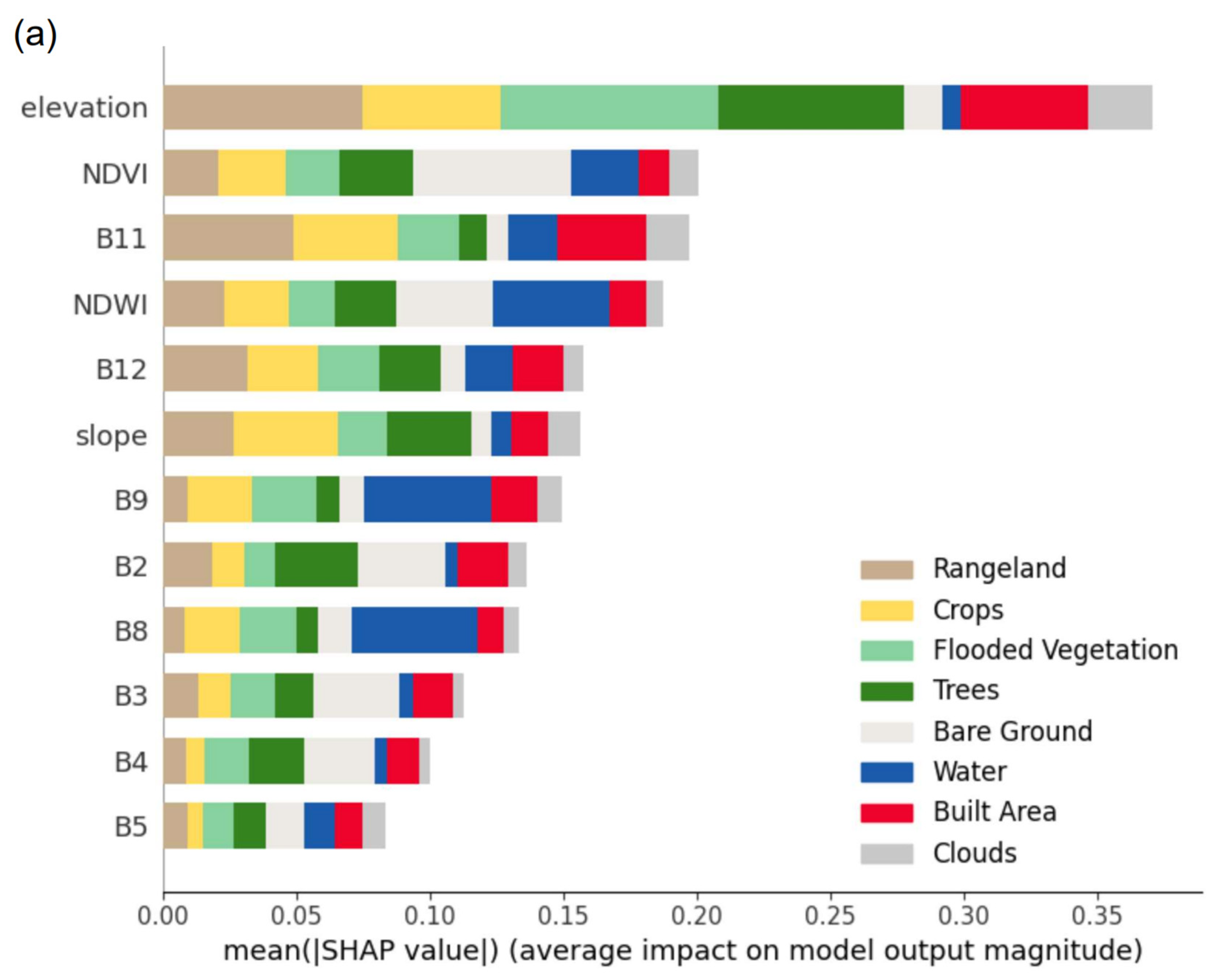
Figure 5 shows the SHAP feature importance computed for the sk-learn’s RF classifier on the testing dataset. Figure 5a shows the global feature importance ranking for all the land cover classes, in which the x-axis is the mean of the absolute SHAP values across all samples. Each row represents the SHAP values for a single feature that is horizontally stacked across all of the classes. The longer the bars, the higher the importance and contribution of the feature. The ranking of the SHAP-value-based feature importance echoes that based on impurity and permutation. According to Figure 5a, the ‘elevation’, ‘NDVI’, ‘B11’, and ‘NDWI’ bands are the top four most important features. They are also largely recognized as important based on both the impurity-based importance and permutation importance. Figure 5b shows the global feature importance (b1) and local explanation summary (b2) plots for a single class of “Water”. Figure 5c shows the global feature importance (c1) and local explanation summary (c2) for the “Bare Ground” class. Similar plots for all other classes are available as well. Note that the SHAP algorithm produces class-level feature importance metrics as opposed to the other two counterparts [22]. For the local summary plot, the x-axis is the SHAP value of a feature for each sample’s possible prediction. The red dots indicate a high value of that feature, while the blue dots represent a low feature value. Figure 5b shows that the ‘B9′ and ‘B8′ bands are the two most important features for the land cover class “Water”, followed by the ‘NDWI’ and ‘NDVI’ bands. According to the local explanation summary plot (Figure 5(b2)), samples with low feature values for bands ‘B9’, ‘B8’, and NDVI and those with high NDWI values contribute positively to the prediction (i.e., class “Water”). For the “Bare Ground” class, ‘NDWI’ and ‘NDVI’ are the two most important features, followed by the three visible B/G/R bands (‘B2/B3/B4’). According to the local explanation summary plot (Figure 5(c2)), high visible band values contribute positively to the class. The impacts of ‘NDWI’ and ‘NDVI’ bands, however, are not as conclusive as those for class ‘Water’. Apart from these plots, the SHAP dependence plots between two features are also available, which show how a feature’s value (x-axis) impacts the prediction (y-axis) of every sample (each dot) in a dataset.
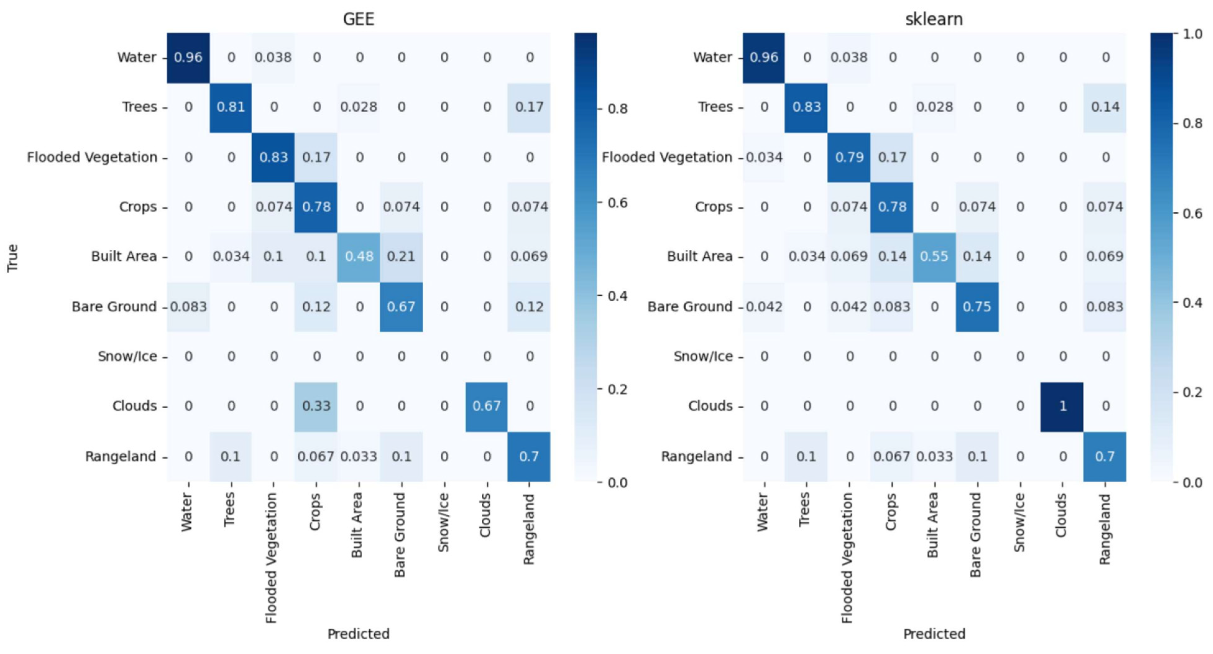
Figure 6 presents the confusion matrix of the GEE and scikit-learn’s random forest classifier, which have an overall accuracy of 0.74 and 0.77, respectively. Note that the training and testing datasets were generated by stratified sampling from Esri’s global land cover product. There are no data points for the ‘Snow/Ice’ class, and there are far fewer data points for the ‘Clouds’ class than for other classes. It is widely accepted that the ability of any supervised classifier to produce accurate maps is limited by the quality and amount of training data, the number and diversity of classes to be mapped, and the predictors (features) chosen to construct the classifier. For future applications, it is suggested to define the land cover classes tailored specifically to the geographical and ecological conditions of the studied area of interest and prepare a sufficient amount of quality training data.

3.2. Land Cover Change off Dubai Coast

One of the main drivers for land cover change is reclamation. Major land reclamation projects, such as the Palm Islands and the World Islands in Dubai, United Arab Emirates, have significantly changed the appearance of the country. This example shows the tool’s capacity to capture land cover changes that occurred over the past two decades for a region off the coast of Dubai. All available bands with Landsat-7 TOA and two spectral indices NDVI and NDWI were selected as the predictor variables. The example dataset provided by [34], which included only two classes “Land” and “Water”, was used to train a random forest classifier. Note that although the classifier reported an accuracy of 1.0, the insufficient sample size may hinder a comprehensive feature importance analysis as conducted for the case studied above. Nevertheless, this case demonstrates decently the land cover change that has been occurring during the past two decades around the Dubai coast (see supporting document for other visualization plots).
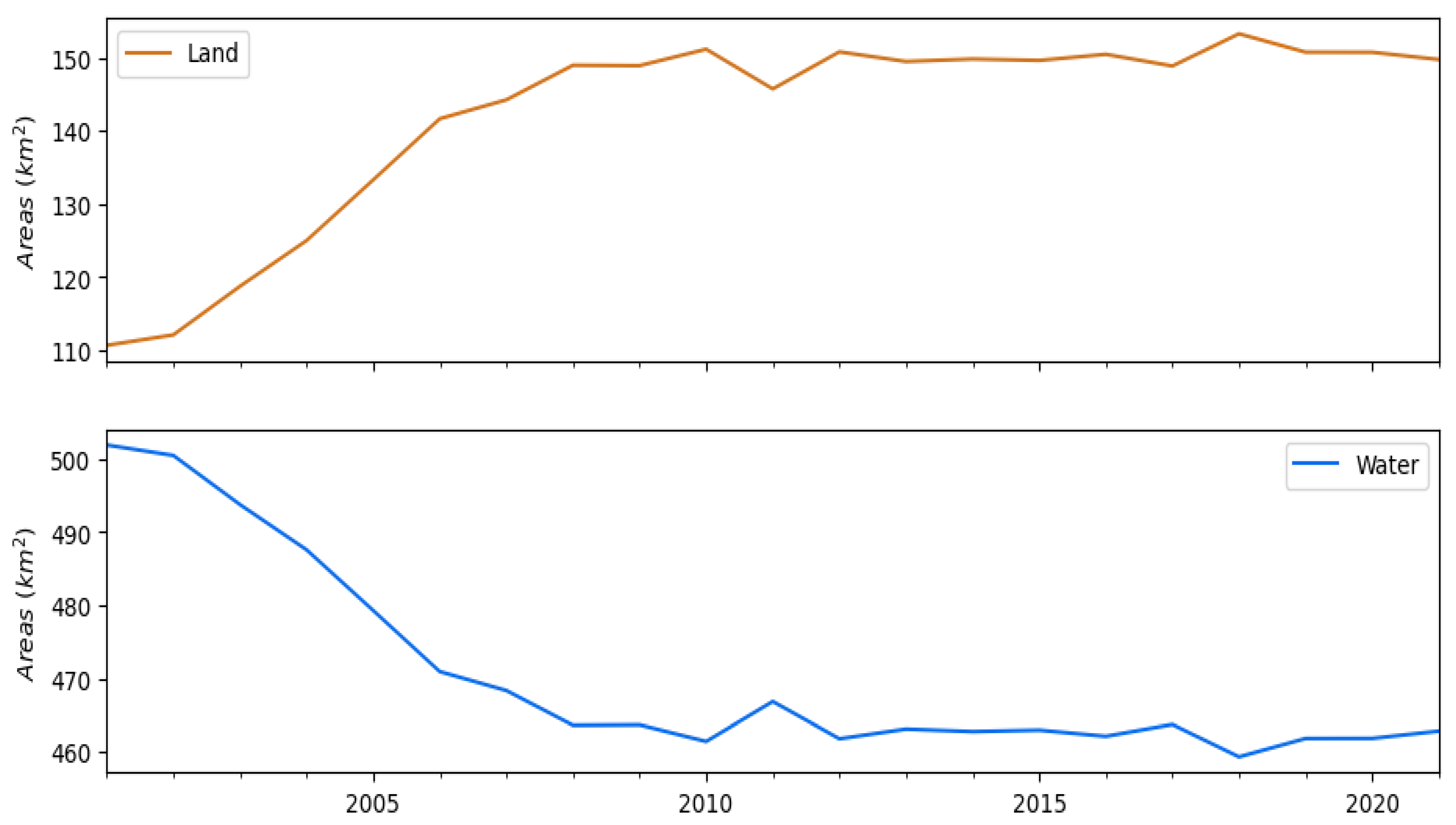
Figure 7 illustrates the spatio-temporal evolution of the land cover change, which confirms that the World Islands were constructed around the same time (about two years later, to be specific) as the Palm Islands. No significant change was observed after the year 2008. Figure 8 shows the zonal areas calculated each year for all of the composite images. A total of about 40 km2 of land was reclaimed along the Dubai coastline between the years 2001 and 2008, and no significant change was seen after the 2008 financial crisis. The area estimates that each land cover class may be further adjusted accounting for the producer’s accuracy (or omission error) and user’s accuracy (or commission error) [32,53]. It should be noted that these spatio-temporal dynamics plots can be generated interactively by selecting the specific years and land cover types of interest. The classified yearly composites can then be exported to other platforms such as ArcGIS or QGIS for other types of land cover change analysis.

4. Concluding Remarks

This paper presented an open-source explainable ML tool by integrating XAI with the workflow of land cover mapping and monitoring using Google Earth Engine. The interactive tool leverages the abundant datasets on GEE and various Python frameworks and accommodates the workflow of both land cover classification and change detection. It boasts an explainable machine learning module to calculate the impurity-based, permutation-based, and SHAP-value-based feature importances, allowing users to assess the classifier and determine the most important features. The tool supports uploading previously labeled data with custom classes and generating labels directly from global land cover products, but it does not yet support online label preparation by manually defining classes and adding samples. Two case studies are presented to demonstrate the capability of the developed tool. The first case study showcases the land cover mapping workflow coupled with a variety of visualization tools—the SHAP values plots in particular. The second case study demonstrates land change monitoring by following the same workflow and using the same user interface. Both the impurity-based and the permutation-based feature importances are traditional global metrics aimed at optimizing the feature space to improve the overall model performance. The local explanation benefits offered by SHAP, however, may provide more mechanistic correlations between machine learning models and their predictions, e.g., by employing the biological, physical, and spectral signatures of the land cover classes to be mapped. While SHAP has been applied to help explain natural hazard susceptibility, its application to multi-label land cover mapping is still scarce but is expected to grow fast in the coming years.
Developed and tested in the Colab environment, users can perform the classification task interactively and iteratively, e.g., by adding more labeled data to the sample input file and/or changing the features list according to the feature importance analysis. While users without coding experience can simply run the classification workflow, users comfortable with coding can customize and expand the functionalities to suit their needs. More satellite datasets, spectral indices, and other machine learning models could also be accommodated [22,36]. State-of-the-art deep learning models that normally report a higher classification accuracy can be integrated as well. This highlights an even more important role XAI can play to help interpret these black-box models. The framework and the user interface can potentially be converted to a web application, which could help to disseminate the research to the applied remote sensing community. The interactive and visual tool may provide a good start and inspire a wide range of researchers to facilitate XAI-empowered remote sensing applications.

Author Contributions

All authors have contributed to this paper. H.C. took the lead in designing and developing the interactive tool and contributed to writing and editing the text. L.Y. initiated the conceptualization, contributed to writing and overall organization, identified selected research to include in the manuscript, provided suggestions for the visualization design, and coordinated input from other authors. Q.W. provided feedback to the interactive tool and edited the text. All authors have revised the manuscript. All authors have read and agreed to the published version of the manuscript.

Funding

This material is partly based upon work supported by the US National Aeronautics and Space Administration under grant number 80NSSC22K1742 and by the funding support at the University of New Mexico from the College of Arts and Sciences, and from the Office of the Vice President for Research WeR1 Faculty Success Program (WeR1 FaST 2022 and WeR1 SuRF 2022).

Data Availability Statement

The code, supplemental documents, and video tutorials are available to the public at https://github.com/GeoAIR-lab/XAI-tool4GEE (accessed on 13 September 2023).

Acknowledgments

The authors are grateful to the reviewers for their useful suggestions.

Conflicts of Interest

The authors declare no conflict of interest.

Abbreviations

The following abbreviations (ordered alphabetically) are used in this article:
AI Artificial Intelligence
ColabGoogle Colaboratory
CSVComma Separated Values
DLDeep Learning
EOEarth Observation
LULCLand Use Land Cover
MDIMean Decrease in Impurity
MLMachine Learning
NANot Applicable
NASAShuttle Radar Topography Mission
NBRNormalized Burn Ratio
NDVINormalized Difference Vegetation Index
NDWINormalized Difference Water Index
PCP Parallel Coordinate Plot
RF Random Forest
RS Remote Sensing
ROI Region Of Interest
SHAPShapley Additive Explanations
SRSurface Reflectance
SRTMShuttle Radar Topography Mission
TOATop-of-Atmosphere
XAI Explainable Artificial Intelligence

References

  1. Meske, C.; Bunde, E.; Schneider, J.; Gersch, M. Explainable Artificial Intelligence: Objectives, Stakeholders, and Future Research Opportunities. Inf. Syst. Manag. 2022, 39, 53–63. [Google Scholar] [CrossRef]
  2. Lary, D.J.; Alavi, A.H.; Gandomi, A.H.; Walker, A.L. Machine Learning in Geosciences and Remote Sensing. Geosci. Front. 2016, 7, 3–10. [Google Scholar] [CrossRef]
  3. Mamalakis, A.; Ebert-Uphoff, I.; Barnes, E.A. Explainable Artificial Intelligence in Meteorology and Climate Science: Model Fine-Tuning, Calibrating Trust and Learning New Science. In xxAI—Beyond Explainable AI: International Workshop, Held in Conjunction with ICML 2020, 18 July 2020, Vienna, Austria, Revised and Extended Papers; Holzinger, A., Goebel, R., Fong, R., Moon, T., Müller, K.-R., Samek, W., Eds.; Springer International Publishing: Cham, Switzerland, 2022; pp. 315–339. ISBN 9783031040832. [Google Scholar]
  4. Wulder, M.A.; Roy, D.P.; Radeloff, V.C.; Loveland, T.R.; Anderson, M.C.; Johnson, D.M.; Healey, S.; Zhu, Z.; Scambos, T.A.; Pahlevan, N.; et al. Fifty Years of Landsat Science and Impacts. Remote Sens. Environ. 2022, 280, 113195. [Google Scholar] [CrossRef]
  5. Yang, L.; Driscol, J.; Sarigai, S.; Wu, Q.; Chen, H.; Lippitt, C.D. Google Earth Engine and Artificial Intelligence (AI): A Comprehensive Review. Remote Sens. 2022, 14, 3253. [Google Scholar] [CrossRef]
  6. Barnes, E.A.; Hurrell, J.W.; Ebert-Uphoff, I.; Anderson, C.; Anderson, D. Viewing Forced Climate Patterns through an AI Lens. Geophys. Res. Lett. 2019, 46, 13389–13398. [Google Scholar] [CrossRef]
  7. Bergen, K.J.; Johnson, P.A.; de Hoop, M.V.; Beroza, G.C. Machine Learning for Data-Driven Discovery in Solid Earth Geoscience. Science 2019, 363, eaau0323. [Google Scholar] [CrossRef] [PubMed]
  8. Karpatne, A.; Ebert-Uphoff, I.; Ravela, S.; Babaie, H.A.; Kumar, V. Machine Learning for the Geosciences: Challenges and Opportunities. IEEE Trans. Knowl. Data Eng. 2019, 31, 1544–1554. [Google Scholar] [CrossRef]
  9. Reichstein, M.; Camps-Valls, G.; Stevens, B.; Jung, M.; Denzler, J.; Carvalhais, N. Prabhat Deep Learning and Process Understanding for Data-Driven Earth System Science. Nature 2019, 566, 195–204. [Google Scholar] [CrossRef]
  10. Gevaert, C.M. Explainable AI for Earth Observation: A Review Including Societal and Regulatory Perspectives. Int. J. Appl. Earth Obs. Geoinf. 2022, 112, 102869. [Google Scholar] [CrossRef]
  11. Minh, D.; Wang, H.X.; Li, Y.F.; Nguyen, T.N. Explainable Artificial Intelligence: A Comprehensive Review. Artif. Intell. Rev. 2022, 55, 3503–3568. [Google Scholar] [CrossRef]
  12. Samek, W.; Montavon, G.; Vedaldi, A.; Hansen, L.K.; Müller, K.-R. Explainable AI: Interpreting, Explaining and Visualizing Deep Learning; Springer Nature: Cham, Switzerland, 2019; ISBN 9783030289546. [Google Scholar]
  13. Yang, G.; Ye, Q.; Xia, J. Unbox the Black-Box for the Medical Explainable AI via Multi-Modal and Multi-Centre Data Fusion: A Mini-Review, Two Showcases and beyond. Inf. Fusion 2022, 77, 29–52. [Google Scholar] [CrossRef]
  14. Barredo Arrieta, A.; Díaz-Rodríguez, N.; Del Ser, J.; Bennetot, A.; Tabik, S.; Barbado, A.; Garcia, S.; Gil-Lopez, S.; Molina, D.; Benjamins, R.; et al. Explainable Artificial Intelligence (XAI): Concepts, Taxonomies, Opportunities and Challenges toward Responsible AI. Inf. Fusion 2020, 58, 82–115. [Google Scholar] [CrossRef]
  15. Adadi, A.; Berrada, M. Peeking Inside the Black-Box: A Survey on Explainable Artificial Intelligence (XAI). IEEE Access 2018, 6, 52138–52160. [Google Scholar] [CrossRef]
  16. Roscher, R.; Bohn, B.; Duarte, M.F.; Garcke, J. Explainable Machine Learning for Scientific Insights and Discoveries. IEEE Access 2020, 8, 42200–42216. [Google Scholar] [CrossRef]
  17. Yang, L.; MacEachren, A.M.; Mitra, P.; Onorati, T. Visually-Enabled Active Deep Learning for (geo) Text and Image Classification: A Review. ISPRS Int. J. 2018, 7, 65. [Google Scholar] [CrossRef]
  18. Hall, O.; Ohlsson, M.; Rögnvaldsson, T. A Review of Explainable AI in the Satellite Data, Deep Machine Learning, and Human Poverty Domain. Patterns 2022, 3, 100600. [Google Scholar] [CrossRef] [PubMed]
  19. Belgiu, M.; Drăguţ, L. Random Forest in Remote Sensing: A Review of Applications and Future Directions. ISPRS J. Photogramm. Remote Sens. 2016, 114, 24–31. [Google Scholar] [CrossRef]
  20. Breiman, L. Random Forests. Mach. Learn. 2001, 45, 5–32. [Google Scholar] [CrossRef]
  21. Lundberg, S.M.; Lee, S.-I. A Unified Approach to Interpreting Model Predictions. In Proceedings of the Advances in Neural Information Processing Systems, Long Beach, CA, USA, 4–9 December 2017. [Google Scholar]
  22. Hosseiny, B.; Abdi, A.M.; Jamali, S. Urban Land Use and Land Cover Classification with Interpretable Machine Learning—A Case Study Using Sentinel-2 and Auxiliary Data. Remote Sens. Appl. Soc. Environ. 2022, 28, 100843. [Google Scholar] [CrossRef]
  23. Iban, M.C.; Bilgilioglu, S.S. Snow Avalanche Susceptibility Mapping Using Novel Tree-Based Machine Learning Algorithms (XGBoost, NGBoost, and LightGBM) with eXplainable Artificial Intelligence (XAI) Approach. Stoch. Environ. Res. Risk Assess. 2023, 37, 2243–2270. [Google Scholar] [CrossRef]
  24. Pradhan, B.; Lee, S.; Dikshit, A.; Kim, H. Spatial Flood Susceptibility Mapping Using an Explainable Artificial Intelligence (XAI) Model. Geosci. Front. 2023, 14, 101625. [Google Scholar] [CrossRef]
  25. Dahal, A.; Lombardo, L. Explainable Artificial Intelligence in Geoscience: A Glimpse into the Future of Landslide Susceptibility Modeling. Comput. Geosci. 2023, 176, 105364. [Google Scholar] [CrossRef]
  26. Gorelick, N.; Hancher, M.; Dixon, M.; Ilyushchenko, S.; Thau, D.; Moore, R. Google Earth Engine: Planetary-Scale Geospatial Analysis for Everyone. Remote Sens. Environ. 2017, 202, 18–27. [Google Scholar] [CrossRef]
  27. Velastegui-Montoya, A.; Montalván-Burbano, N.; Carrión-Mero, P.; Rivera-Torres, H.; Sadeck, L.; Adami, M. Google Earth Engine: A Global Analysis and Future Trends. Remote Sens. 2023, 15, 3675. [Google Scholar] [CrossRef]
  28. Hansen, M.C.; Potapov, P.V.; Moore, R.; Hancher, M.; Turubanova, S.A.; Tyukavina, A.; Thau, D.; Stehman, S.V.; Goetz, S.J.; Loveland, T.R.; et al. High-Resolution Global Maps of 21st-Century Forest Cover Change. Science 2013, 342, 850–853. [Google Scholar] [CrossRef] [PubMed]
  29. Pekel, J.-F.; Cottam, A.; Gorelick, N.; Belward, A.S. High-Resolution Mapping of Global Surface Water and Its Long-Term Changes. Nature 2016, 540, 418–422. [Google Scholar] [CrossRef]
  30. Koo, Y.; Xie, H.; Mahmoud, H.; Iqrah, J.M.; Ackley, S.F. Automated Detection and Tracking of Medium-Large Icebergs from Sentinel-1 Imagery Using Google Earth Engine. Remote Sens. Environ. 2023, 296, 113731. [Google Scholar] [CrossRef]
  31. Wu, Q. Geemap: A Python Package for Interactive Mapping with Google Earth Engine. J. Open Source Softw. 2020, 5, 2305. [Google Scholar] [CrossRef]
  32. Gatis, N.; Carless, D.; Luscombe, D.J.; Brazier, R.E.; Anderson, K. An Operational Land Cover and Land Cover Change Toolbox: Processing Open-source Data with Open-source Software. Ecol. Solut. Evid. 2022, 3, e12162. [Google Scholar] [CrossRef]
  33. Buscombe, D.; Goldstein, E.B. A Reproducible and Reusable Pipeline for Segmentation of Geoscientific Imagery. Earth Space Sci. 2022, 9, e2022EA002332. [Google Scholar] [CrossRef]
  34. Murray, N.J.; Keith, D.A.; Simpson, D.; Wilshire, J.H.; Lucas, R.M. Remap: An Online Remote Sensing Application for Land Cover Classification and Monitoring. Methods Ecol. Evol. 2018, 9, 2019–2027. [Google Scholar] [CrossRef]
  35. Xing, H.; Hou, D.; Wang, S.; Yu, M.; Meng, F. O-LCMapping: A Google Earth Engine-Based Web Toolkit for Supporting Online Land Cover Classification. Earth Sci. Inf. 2021, 14, 529–541. [Google Scholar] [CrossRef]
  36. Temenos, A.; Temenos, N.; Kaselimi, M.; Doulamis, A.; Doulamis, N. Interpretable Deep Learning Framework for Land Use and Land Cover Classification in Remote Sensing Using SHAP. IEEE Geosci. Remote Sens. Lett. 2023, 20, 1–5. [Google Scholar] [CrossRef]
  37. Ipywidgets: Interactive Widgets for the Jupyter Notebook. Available online: https://github.com/jupyter-widgets/ipywidgets (accessed on 27 July 2023).
  38. Ipyleaflet: A Jupyter—Leaflet.js Bridge. Available online: https://github.com/jupyter-widgets/ipyleaflet (accessed on 27 July 2023).
  39. Pedregosa, F.; Varoquaux, G.; Gramfort, A.; Michel, V.; Thirion, B.; Grisel, O.; Blondel, M.; Prettenhofer, P.; Weiss, R.; Dubourg, V.; et al. Scikit-Learn: Machine Learning in Python. J. Mach. Learn. Res. 2011, 12, 2825–2830. [Google Scholar]
  40. Shap: A Game Theoretic Approach to Explain the Output of Any Machine Learning Model. Available online: https://github.com/shap/shap (accessed on 27 July 2023).
  41. Farr, T.G.; Rosen, P.A.; Caro, E.; Crippen, R. The Shuttle Radar Topography Mission. Rev. Geophys. 2007, 45, RG2004. [Google Scholar] [CrossRef]
  42. Zanaga, D.; Van De Kerchove, R.; De Keersmaecker, W.; Souverijns, N.; Brockmann, C.; Quast, R.; Wevers, J.; Grosu, A.; Paccini, A.; Vergnaud, S.; et al. ESA WorldCover 10 M 2020 v100. 2021. Available online: https://zenodo.org/record/5571936 (accessed on 13 September 2023).
  43. Zanaga, D.; Van De Kerchove, R.; Daems, D.; De Keersmaecker, W.; Brockmann, C.; Kirches, G.; Wevers, J.; Cartus, O.; Santoro, M.; Fritz, S.; et al. ESA WorldCover 10 M 2021 v200. 2022. Available online: https://zenodo.org/record/7254221 (accessed on 13 September 2023).
  44. Karra, K.; Kontgis, C.; Statman-Weil, Z.; Mazzariello, J.C.; Mathis, M.; Brumby, S.P. Global Land Use / Land Cover with Sentinel 2 and Deep Learning. In Proceedings of the 2021 IEEE International Geoscience and Remote Sensing Symposium IGARSS, Brussels, Belgium, 11–16 July 2021; pp. 4704–4707. [Google Scholar]
  45. Brown, C.F.; Brumby, S.P.; Guzder-Williams, B.; Birch, T.; Hyde, S.B.; Mazzariello, J.; Czerwinski, W.; Pasquarella, V.J.; Haertel, R.; Ilyushchenko, S.; et al. Dynamic World, Near Real-Time Global 10 M Land Use Land Cover Mapping. Sci. Data 2022, 9, 1251. [Google Scholar] [CrossRef]
  46. Venter, Z.S.; Barton, D.N.; Chakraborty, T.; Simensen, T.; Singh, G. Global 10 M Land Use Land Cover Datasets: A Comparison of Dynamic World, World Cover and Esri Land Cover. Remote Sens. 2022, 14, 4101. [Google Scholar] [CrossRef]
  47. ee.Classifier.smileRandomForest|Google Earth Engine|Google for Developers. Available online: https://developers.google.com/earth-engine/apidocs/ee-classifier-smilerandomforest (accessed on 27 July 2023).
  48. Scikit-Learn: Scikit-Learn: Machine Learning in Python. Available online: https://github.com/scikit-learn/scikit-learn (accessed on 27 July 2023).
  49. Mahdianpari, M.; Jafarzadeh, H.; Granger, J.E.; Mohammadimanesh, F.; Brisco, B.; Salehi, B.; Homayouni, S.; Weng, Q. A Large-Scale Change Monitoring of Wetlands Using Time Series Landsat Imagery on Google Earth Engine: A Case Study in Newfoundland. GISci. Remote Sens. 2020, 57, 1102–1124. [Google Scholar] [CrossRef]
  50. Amani, M.; Kakooei, M.; Ghorbanian, A.; Warren, R.; Mahdavi, S.; Brisco, B.; Moghimi, A.; Bourgeau-Chavez, L.; Toure, S.; Paudel, A.; et al. Forty Years of Wetland Status and Trends Analyses in the Great Lakes Using Landsat Archive Imagery and Google Earth Engine. Remote Sens. 2022, 14, 3778. [Google Scholar] [CrossRef]
  51. Zhao, F.; Feng, S.; Xie, F.; Zhu, S.; Zhang, S. Extraction of Long Time Series Wetland Information Based on Google Earth Engine and Random Forest Algorithm for a Plateau Lake Basin—A Case Study of Dianchi Lake, Yunnan Province, China. Ecol. Indic. 2023, 146, 109813. [Google Scholar] [CrossRef]
  52. León-Pérez, M.C.; Reisinger, A.S.; Gibeaut, J.C. Spatial-Temporal Dynamics of Decaying Stages of Pelagic Sargassum Spp. along Shorelines in Puerto Rico Using Google Earth Engine. Mar. Pollut. Bull. 2023, 188, 114715. [Google Scholar] [CrossRef]
  53. Olofsson, P.; Foody, G.M.; Herold, M.; Stehman, S.V.; Woodcock, C.E.; Wulder, M.A. Good Practices for Estimating Area and Assessing Accuracy of Land Change. Remote Sens. Environ. 2014, 148, 42–57. [Google Scholar] [CrossRef]
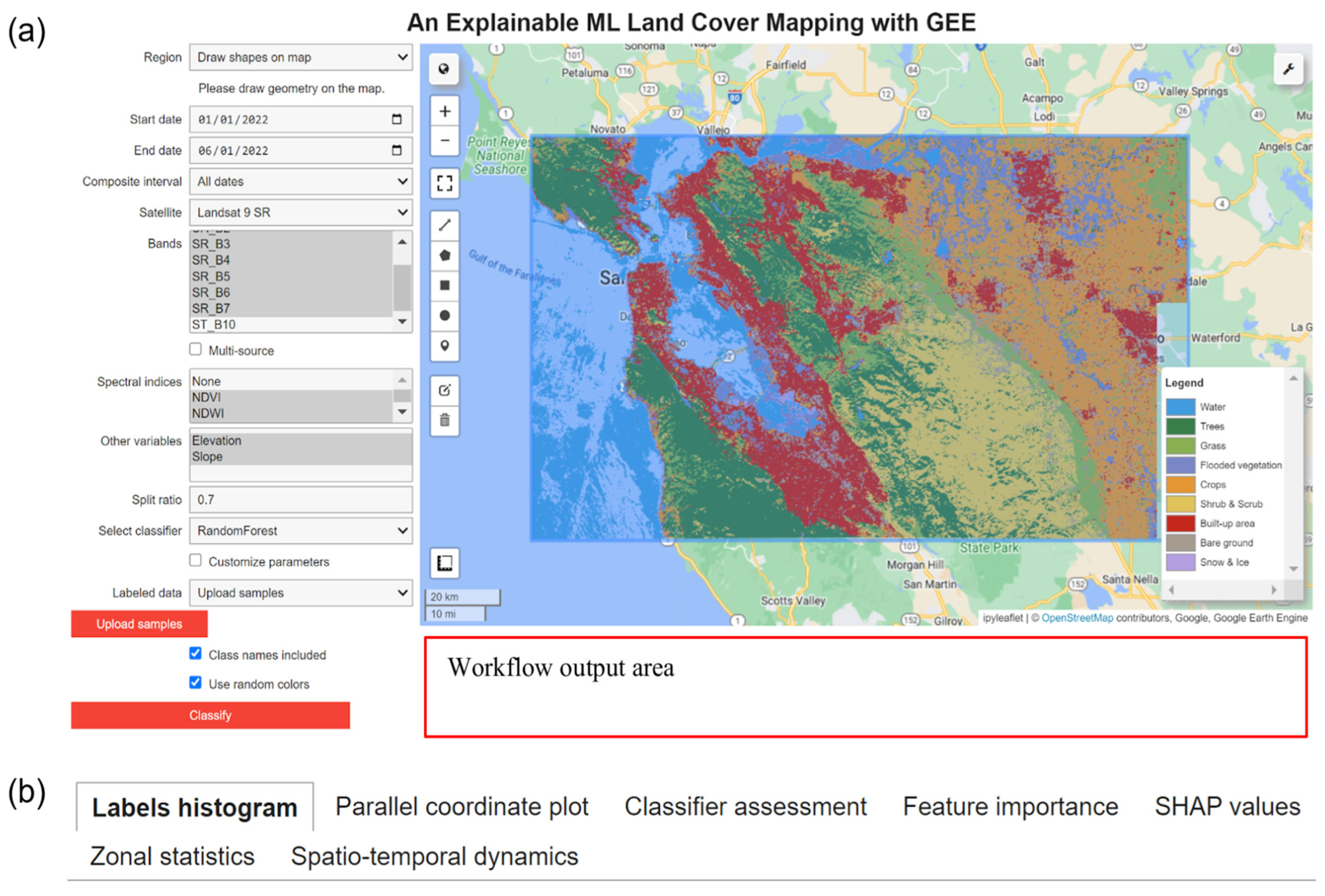
Figure 1. The user interface of the land cover mapping tool running on Colab. (a) User input area (left) and interactive ipyleaflet map (right). (b) Various tabs displaying the classification results.
Remotesensing 15 04585 g001
Figure 2. Workflow chart of the land cover mapping tool developed and to be run on Colab.
Remotesensing 15 04585 g002
Figure 3. Demonstration of land cover classification around San Francisco Bay, USA. (a) Natural color (red/green/blue) composite image (Sentinel-2 Level2-A). (b) Training (circles) and testing (triangles) sample data. (c) Classification result. Note that the same class palette was used for both the sample data (b) and the classified map (c).
Remotesensing 15 04585 g003
Figure 4. Feature importance plots. (a) GEE and sk-learn impurity-based feature importance. (b) sk-learn permutation-based feature importance.
Remotesensing 15 04585 g004
Figure 5. SHAP values plots for all of the testing samples. (a) Global feature importance for all of the land cover classes. (b1,b2) Global feature importance and local explanation summary for class “Water”. (c1,c2) Global feature importance and local explanation summary for class “Bare Ground”.
Remotesensing 15 04585 g005aRemotesensing 15 04585 g005b
Figure 6. Confusion matrix for the GEE (left) and scikit-learn (right) random forest classifier.
Remotesensing 15 04585 g006
Figure 7. Spatio-temporal land cover change off the coast of Dubai, United Arab Emirates, which shows that the commencement of the World Islands construction was about two years later than that of the Palm Islands.
Remotesensing 15 04585 g007
Figure 8. Zonal areas calculated for each classified yearly composite image off the coast of Dubai. A large amount of land was reclaimed before 2008.
Remotesensing 15 04585 g008
Table 1. Satellite/band information and spectral indices available for land cover classification.
SatelliteImage Collection ID in GEEBandsDate Availability
L7 SRLANDSAT/LE07/C02/T1_L2SR_B1–SR_B5, SR_B7, ST_B628 May 1999–29 March 2023
L7 TOALANDSAT/LE07/C02/T1_TOAB1–B5, B7–B828 May 1999–29 March 2023
L8 SRLANDSAT/LC08/C02/T1_L2SR_B1–SR_B7, ST_B10April 2013–Present
L8 TOALANDSAT/LC08/C02/T1_TOAB1–B11April 2013–Present
L9 SRLANDSAT/LC09/C02/T1_L2SR_B1–SR_B7, ST_B10October 2021–Present
L8 TOALANDSAT/LC09/C02/T1_TOAB1–B11October 2021–Present
Sentinel-2 SR Level-2ACOPERNICUS/S2_SR_HARMONIZEDB1–B12, B8A28 March 2017–Present
Sentinel-2 TOA Level-1CCOPERNICUS/S2_HARMONIZEDB1–B12, B8A23 June 2015–Present
Spectral indicesNDVI, NDWI, NBRNANA
Topographic variablesUSGS/SRTMGL1_003Elevation (slope)11 February 2000–22 February 2000
NA: Not applicable.
Disclaimer/Publisher’s Note: The statements, opinions and data contained in all publications are solely those of the individual author(s) and contributor(s) and not of MDPI and/or the editor(s). MDPI and/or the editor(s) disclaim responsibility for any injury to people or property resulting from any ideas, methods, instructions or products referred to in the content.