SGOT: A Simplified Geometric-Optical Model for Crown Scene Components Modeling over Rugged Terrain

Abstract

Topography affects the fraction of scene components of the canopy and background, resulting in the observed reflectance distortion. Modeling the canopy reflectance over rugged terrain needs to account for topographic effects. For this purpose, the existing models greatly increased the mathematical complexity while improving description of terrain and crown structure, which dramatically decreased the computational efficiency so as to limit their universal application. In this study, we developed a simplified geometric-optical model (SGOT) for simulating the scene components over rugged terrain. The geotropism of tree growth was considered to make SGOT physically sound. The internal structure of crown was simplified to make SGOT mathematically simpler. Scene component observations derived from Persistence of Vision Ray-tracer (POV-Ray) on surfaces with different normal directions and simulations were made using Geometric-Optical and Mutual Shadowing Coupled with Topography Model (GOMST) and Geometric-Optical for Sloping Terrains Model GOST; models were combined to test the SGOT model. In addition, topographic factors and crown density effect on the scene components modeling were analyzed. The results indicated that SGOT has good accuracy (R² for the areal proportions of sunlit crown (Kc), sunlit background (Kg), shaded crown (Kt), and shaded background (Kz) are 0.853, 0.857, 0.914, and 0.838, respectively) compared with POV-Ray simulation, and performs better than GOMST, especially in scenes with high crown density. Moreover, SGOT outperformed the compared models in computational efficiency (4% faster than GOMST and 29.5% faster than GOST). Finally, the simulations of the scene components distribution in different topographic factors and crown density were further discussed. SGOT and GOST can both capture scene component variations caused by terrain better than GOMST, but comparatively, SGOT provides a more efficient tool to simulate the crown scene components because of its physical soundness and mathematical simplicity, and consequently, it will facilitate the modeling of canopy reflectance over mountainous regions.

1. Introduction

Canopy reflectance models provide causal relationships between the vegetation structural parameters and remote sensing observations, and they have served as effective tools to explore biophysical variables from remote sensing observations [1], including radiative transfer (RT) [2,3], geometric-optical (GO) [4,5], hybrid GO-RT [6,7], and computer simulation models [8,9]. For geometric-optical (GO) models, the observed reflected signals are composed of scattering contributions from canopy and background in sunlight and shadow, which are called crown scene components that are the key parameters to control the area fraction of different radiation-scattering components [4,10]. However, with the variations of the surface normal direction, the fraction of the crown scene components of sloping terrain is different from that of flat terrain. Many studies have shown that complex terrains can significantly influence the crown scene components [11,12,13,14]. Firstly, the increase of the slope can alter both the illumination and view angles; the reflected radiance is affected by the surface anisotropic reflectance [15,16]. Secondly, the gap fraction is altered by rugged terrain because the topography can change the direct and diffuse radiation received by the ground surface [17,18]. Therefore, topography regulates incident radiation by changing the upper boundary condition of the radiative transfer process, which affects the radiation received by each scene component and the projection area of each scattering component in the view direction. This should lead the canopy reflectance models to perform poorly in mountainous regions without considering the topographic effects [19,20].

Obviously, accurate simulation of crown scene components under the various terrain conditions is helpful to clarify the transmission and interaction of radiation in crown scene, and plays a decisive role for canopy reflectance model development in the calculation of canopy reflectance. However, reality is always more complex than any model can characterize, and one must perform some abstraction, simplification, and approximation when representing terrestrial scenarios [21]. Over the last three decades, a number of canopy reflectance models which can simulate the scene components have been developed. The scene components firstly appeared in the GO model in 1985 [4], and Li and Strahler (1992) further extended the GO model by considering the mutual shadowing between the crowns (GOMS model) [5]. In the Li–Strahler GO model, the distribution of the forest stand was assumed to be random, and the crown was defined as an opaque body. Chen and Leblanc (1997) established the 4-scale GO model (Four-Scale Bidirectional Reflectance Model) that considered the four scales of crown architecture (i.e., tree groups, tree crowns, branches, and shoots) [10], and further improved the performances of scene components and canopy reflectance simulation. To explore the application of the models in mountainous regions, several GO-like physical canopy reflectance models over rugged terrain were developed. For instance, Schaaf et al. (1994) extended the Li–Strahler GOMS model to sloping terrain (GOMST) by rotating transformation from a horizontal surface to a sloping surface [22]. However, the GOMST model neglected the geotropic nature of tree growth and within-canopy gaps. Fan et al. (2014) extended the 4-scale GO model to sloping terrain (GOST) by establishing a three-dimensional (3-D) crown projection algorithm and using the ray-tracing method [17]. The geotropic nature of tree growth and within-canopy gaps was considered in the GOST model. Subsequently, Fan et al. (2015) proposed the GOST2 model based on the GOST model to improve performance when simulating sunlit crown and shaded crown components [23]. However, the ray-tracing procedure [24] in GOST and GOST2 models was practically limited by computing resources and its accuracy would depend on the amount of structural detail included in the preset scene [25]; the computational demand and the complex 3-D structure dramatically limit their application. Wu et al. (2019) proposed the GOSAILT model [26] by coupling the Li–Strahler GOMS model and the Scattering-from-Arbitrarily-Inclined-Leaves model [21], in which the geotropic nature of tree growth was incorporated in the scene components simulation. However, neglecting the gap fraction within crowns can lead to an overestimation of the areal proportion simulations from crown, particularly for dense vegetation cover.

In summary, the GO-like models over sloping terrain can be divided into the Li–Strahler GO-theory-based models (e.g., GOMST and GOSAILT) and the 4-scale GO-theory-based models (e.g., GOST and GOST2). The former have the advantages of simple internal structure and being easy to implement, but their physical mechanisms are not complete. Neglect of the geotropic nature of tree growth and within-canopy gaps will affect the areal proportion simulations of scattering contributions from crown and background, which can lead to large uncertainties in the follow-up works [27]. The crown structure assumed in the latter models was considered to be most similar to the real forest crown [28]. However, the real 3-D structure of the tree crowns seriously reduces computational efficiency and limits their implementation and application [23,29]. Therefore, a good balance between simulation accuracy and computational efficiency is required in the development of the crown scene components simulation model.

In this paper, we presented a simplified geometric-optical model for crown scene components over rugged terrain based on extension of the GOMST model (hereafter referred to as the SGOT model), in which geotropism of tree growth and gap fraction within crowns were taken into account, and we ensured that the mechanism would be complete as well as easy to implement. To verify the feasibility of the model, we compared the simulation scene components of the SGOT model and POV-Ray over the surfaces of different normal directions. The variations of the scene components over rugged terrains are related to the canopy structure parameters and topographic factors; in particular, slope, aspect, and crown density were recognized as the main factors affecting the scene components simulation. This paper also compared the simulation accuracy and computational efficiency of the SGOT model with the GOMST and GOST models. The development of the SGOT model is described in Section 2. The design of the experiment is given in Section 3. The validation results and analysis are given in Section 4, followed with the discussion in Section 5 and a conclusion in Section 6.

2. SGOT Model Development

According to the GO-like model [4], the forest canopy reflected signals received by sensors are modeled as the sum of the reflectance of individual components weighted by their areas within the pixel:

$$\rho =C\cdot Kc+G\cdot Kg+T\cdot Kt+Z\cdot Kz$$

(1)

where Kc, Kg, Kt, and Kz represent the areal proportions of four crown scene components, i.e., sunlit crown, sunlit background, shaded crown, and shaded background, respectively; C, G, T, and Z are the reflectance factors of four scene components. The derivation of areal proportions of scene components is the key step for canopy reflectance simulation.

In the proposed model, a new projection algorithm of tree crowns on the sloping surface is established, which can retain the geotropism of tree growth. In particular, the tree crown on a sloping surface is represented as a volume consisting of numerous discrete leaves; therefore, the gap fraction is a crucial variable to determine the sunlit components. Unlike the GOMST model, in which the crown is treated as an opaque rigid body, the new model needs to consider the gap fraction within crowns. Here, we referred to the gap fraction formula in the GOST model, which is computed from input parameters such as leaf area index and extinction coefficient.

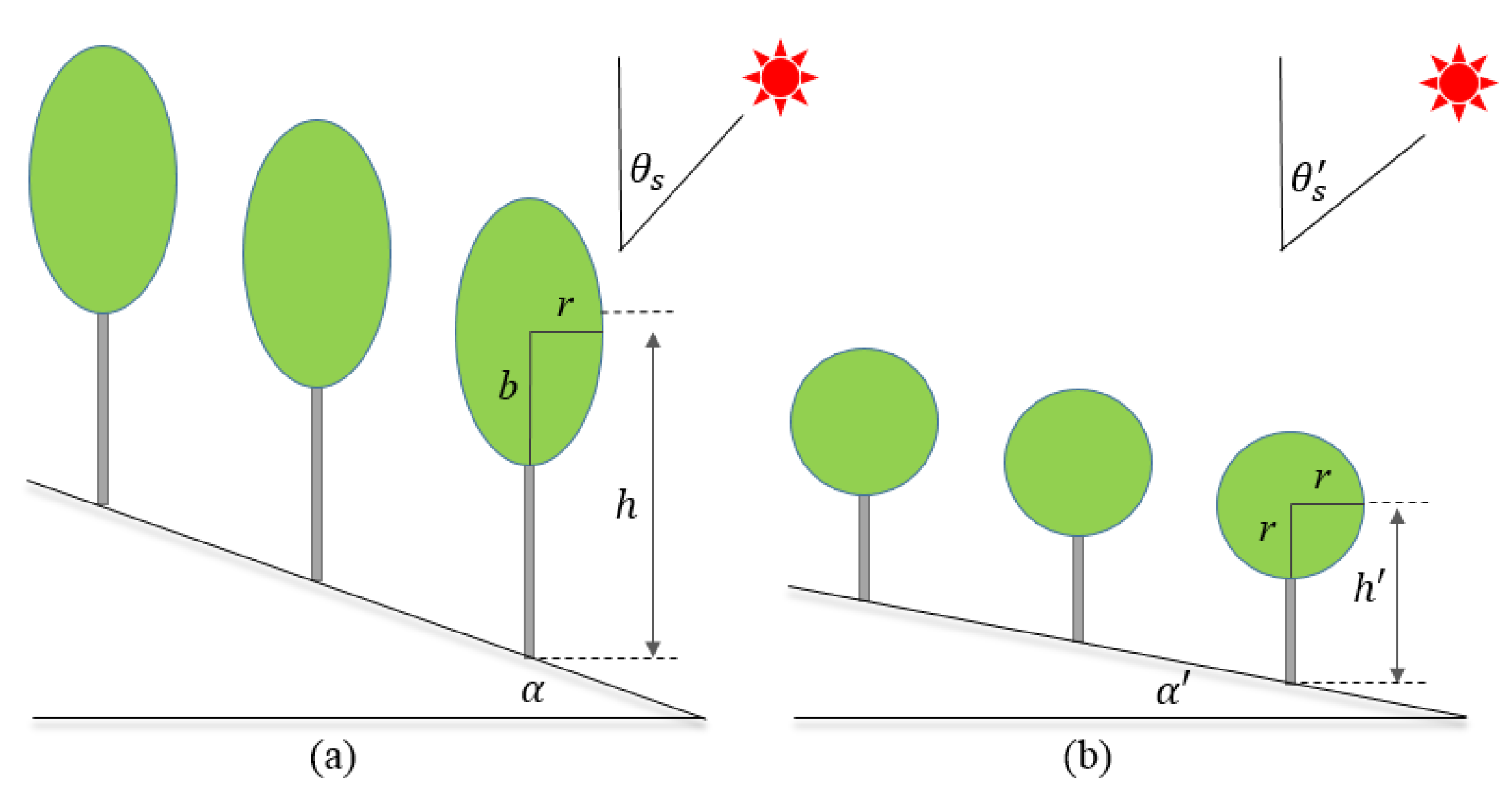
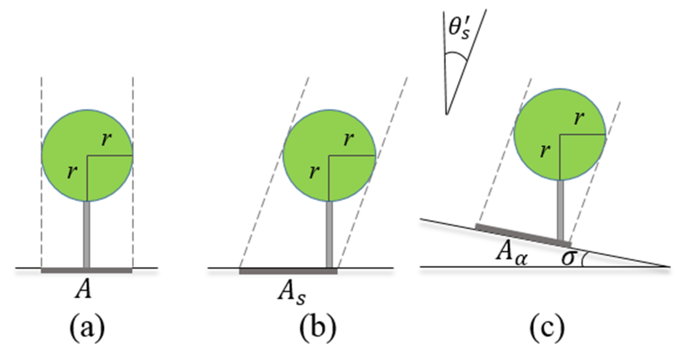
2.1. Crown Shape Transformations

According to the GO model derivation, the shape of a tree was generally assumed to be an ideal 3-D geometric shape according to the geometric characteristics of tree species [5,10,17,23,30]. For example, the “cone + cylinder” crown shape was assumed in the GOST model [17], and the ellipsoidal crown shape was assumed in the GOMST model [22]. The GOST model can be adapted to different crown shapes by adjusting the calculation formula of the crown projected area. However, the GOMST model can only be applicable to simulate the scene components of ellipsoid-shaped tree crowns. Considering that the proposed model needs to be compared with GOMST and GOST models, to facilitate the comparison among different models, the ellipsoidal crown shape was assumed in SGOT and GOST models in this study.

The computation of the canopy projected area over a sloping surface contains two steps, including the crown shape transformation and the projected area topographic transformation. The first step is scene stretching (Figure 1); the purpose of this step is to change the crown shape into a sphere, to facilitate the calculation of the crown projected area. The scene stretching can alter all the geometric parameters in the same ratio of major axis to minor axis (b/r); therefore, it has no effect on the simulation of scene components [5,26]. The second step is to establish the mathematical relationship between the vertically projected area on a horizontal surface and the projected area on a sloping surface. After scene stretching, the ratio of major axis to minor axis is converted from b: r to r: r. Then, the ellipsoid crown is replaced with spheres that cast the same shadow area. The solar zenith angle θ_s and the slope angle α will be changed in the above steps, and the equations are as following [22]:

$${\theta }_s^{\prime }={\tan }^{-1}\left(\frac{b}{r}\tan {\theta }_s\right)$$

(2)

$${\alpha }^{\prime }={\tan }^{-1}\left(\frac{r}{b}\tan \alpha \right)$$

(3)

$$h^{\prime }=\frac{r}{b}h$$

(4)

where θ_s and ${\theta }_s^{\prime }$ are the solar zenith angles before and after scene stretching; b and r are the major and minor axes of the ellipsoid crown; after scene stretching to spherical crown shape, b equals r (Figure 1b); α and α′ are the slope angles before and after scene stretching. Similarly, using the view zenith angle θ_v instead of θ_s, Equation (2) can also be used to calculate the view zenith angle ${\theta }_v^{\prime }$ after scene stretching. h and h′ are the mean height of the crown center before and after scene stretching.

2.2. Projection of Tree Crowns over Sloping Surfaces

The projection of tree crowns is the foundation of scene components simulation. In the SGOT model, we designed a new projection relationship between the vertically projected area on horizontal surface and the projected area on sloping surface (as shown in Figure 2); the projected area in the sunlight direction can be defined as:

$$A_{\alpha }=\{\begin{array}{cc}A{\cos }^{-1}{\theta }_s^{\prime }\cos \sigma & ,0^{°}\le \left|{\phi }_s-{\phi }_{\alpha }\right|\le {90}^{°}\\ A{\cos }^{-1}{\theta }_s^{\prime }{\cos }^{-1}\sigma & ,{90}^{°}<\left|{\phi }_s-{\phi }_{\alpha }\right|\le {180}^{°}\end{array}$$

(5)

$$\tan \sigma =-\cos \left({\phi }_s-{\phi }_{\alpha }\right)\tan \alpha$$

(6)

where A is the vertically projected area on the horizontal surface; A_α is the projected area on the sloping surface; φ_s and φ_α are solar azimuth angle and aspect; σ is the local slope angle, which refers to the included angle formed by the intersection line of the observation plane with the horizontal ground and the sloping surface [31]. The local slope angle contains effective information about slope, aspect, and solar/view azimuth angle; it is newly introduced into the crown projection method in SGOT, suitable for calculating the directional projection area of crowns. One must replace subscript s with v; Equations (5) and (6) can also give the projected area and the local slope angle in the observation direction, respectively.

Compared to the coordinate transformation method adopted by GOMST, the new projection transformation method in SGOT has two advantages. First, it considers the geotropic nature of tree growth; second, the steps of establishing slope coordinate systems and recalculating the incident and observation angles of slope coordinate system are omitted. According to Equation (5), the topography transformations contain two steps: firstly converting vertical projection to incident/observation projection (Figure 2a,b), and secondly, converting the horizontal projection of the incident/observation direction to the sloping projection of the incident/observation direction (Figure 2b,c).

It is generally known that crown shape simply assumed to be the ellipsoidal crown shape will significantly limit its practical application because the natural crowns have various shapes. To facilitate the comparison between SGOT and GOMST, in this experiment, we only assumed that the crown is ellipsoid. By adjusting the horizontal projected area in Equation (5) and introducing the shape-adjusting factor (for the details, please see Equations (A1)–(A3) in Appendix A), other geometric shapes can also be used to replace it in SGOT if needed.

2.3. Crown Gap Fraction over Sloping Surfaces

The variation of gap fraction over sloping surfaces affects the upper boundary condition of the radiative transfer process within a canopy through redistributing the incident irradiance [32]. Introducing a simplified gap fraction as a critical intermediate variable into the SGOT model is considered to be a clear improvement on modeling crown scene components. In the view direction, the gap fraction between crowns (P_{vg_b}) over sloping surfaces can be defined as [17]:

$$P_{vg\_b}=1-D\pi r^2/S$$

(7)

where S is the projection area of the sloping surface in the view direction; D is the number of trees in a pixel; r is the radius of the crown.

In this paper, we defined the distribution of trees as being randomly in space and assumed the canopies to be the “turbid medium” filled with randomly distributed leaves. Therefore, according to Lambert–Beer’s law, the gap fraction within a tree crown (P_{vg_i}) in the view direction can be represented as [33]:

$$P_{vg\_i}=\exp [-K\left({\theta }_v^{\prime },{\phi }_v\right)L_0]$$

(8)

where L₀ is the leaf area index in the view direction, K is the extinction coefficient in the view direction, and can be written as:

$$K\left({\theta }_v^{\prime },{\phi }_v\right)=G\left({\theta }_v^{\prime },{\phi }_v\right)\overline{l}\left({\theta }_v^{\prime },{\phi }_v\right)$$

(9)

where G is the leaf projection function [3] defined as the area of a unit LAI projected along the view direction, and $\overline{l}$ is the mean of path length through a tree crown. In the view direction, it is calculated by the ratio of the volume of crown to the projected area in the view direction:

$$\overline{l}\left({\theta }_v^{\prime },{\phi }_v\right)=4D\pi r^3/3A\cos ({\theta }_v^{\prime })$$

(10)

Therefore, the total gap fraction over a sloping surface in the view direction (P_vg) can be represented as the sum of gap fraction between crowns and within crowns:

$$P_{vg}={\displaystyle \sum _{i=1}^D{P}_{vg\_i}}+P_{vg\_b}$$

(11)

With solar zenith angle ${\theta }_s^{\prime }$ instead of view zenith angle ${\theta }_v^{\prime }$ in the above equations, Equation (10) can be used to calculate the total gap fraction over a sloping surface in the sunlight direction (P_sg).

2.4. Areal Proportions of Scene Components over Sloping Surfaces

According to the GOMST model derivation [22], the scene components of the background consist of the projections of sunlit and shaded background area in the view direction. In particular, the shaded background may be obscured by the crowns in the view direction; the overlap between the sunlight shadow and the observing shadow is given as:

$$O({\theta }_s^{\prime },{\theta }_v^{\prime },{\phi }_{sv})=\frac{1}{\pi }(t-\sin t\cos t)(\sec {\theta }_s^{\prime }+\sec {\theta }_v^{\prime })$$

(12)

where t is given as [5]:

$$\cos t=\frac{h^{\prime }\left|\tan {\theta }_s^{\prime }-\tan {\theta }_v^{\prime }\cos {\phi }_{sv}\right|}{r\left(\sec {\theta }_s^{\prime }+\sec {\theta }_v^{\prime }\right)}$$

(13)

where φ_sv is the relative azimuth angle between the sun and the sensor, h′ is mean height of crown center after scene stretching, r is the radius of the crown after scene stretching. Therefore, using Boolean theory [34] and considering the gap fraction within crowns, the areal proportions of sunlit background and shaded background can be defined as:

$$Kg=\exp \left\{-\lambda \pi r^2\left[\sec {\theta }_s^{\prime }+\sec {\theta }_v^{\prime }-O({\theta }_s^{\prime },{\theta }_v^{\prime },{\phi }_{sv})\right]\right\}+P_{sg\_i}{P}_{vg}$$

(14)

$$Kz=P_{vg}-Kg$$

(15)

where λ is the crown count density, defined as the ratio of the number of tree crowns in a pixel to the area of the pixel, P_{sg_i} is the gap fraction within crowns in the solar direction. With Kg defined, the mutual shadowing factor f can be used to establish a relationship with Kc and Kg. The mutual shadowing factor f is given as:

$$f=\frac{Kc}{1-Kg}$$

(16)

The derivation of f can be found in previous studies [5,22]. Finally, with Kc defined, Kt is given as:

$$Kt=1-Kc-P_{vg}$$

(17)

3. Experimental Setting and Design

3.1. Strategy for Evaluating the Performance of the SGOT Model

The evaluation of the results of crown scene components modeling over sloping surfaces is still a great challenge, because the measurement in real forests is very difficult and expensive [17]. The computer graphics technique provides us with a feasible verification method [23]. It is used to construct the 3-D virtual crowns, and then the information about the crowns and background can be retrieved from the multi-angle observation images of forest scenes [35]. In this study, the computer 3-D virtual model Persistence of Vision Ray-tracer (POV-Ray) was used to construct the 3-D virtual crowns and then to compare the crown scene components with those of the simulation by the proposed model over sloping surfaces. At first, taking the simulated 3-D virtual scenes by POV-Ray as the reference, we evaluated the performance of the SGOT model in crown scene components simulation. The simulation accuracy of the SGOT model can be quantified by the determination coefficients (R²) and root-mean-square error (RMSE). Then, the mechanism correctness of the SGOT model was analyzed according to the basic GO physical principle; for example, the characteristics of scene components should change with topographic factors and view directions, e.g., the hotspot phenomenon [36]. In addition, to reveal the improvement of the SGOT model, two classical GO-like modes (GOMST and GOST) were selected to compare with SGOT on crown scene components simulation; the advantages and disadvantages of the compared models under different conditions were discussed. Considering the simplified scheme adopted in SGOT, the improvement of the calculation efficiency of the SGOT model was also evaluated subsequently.

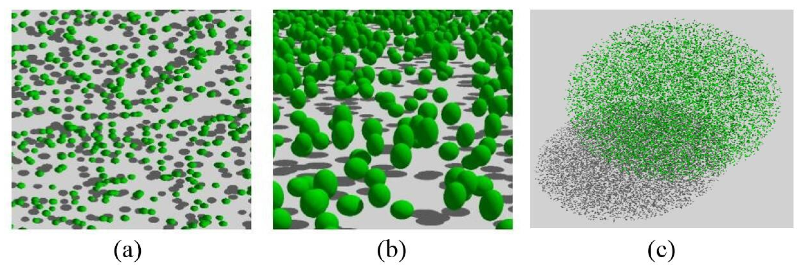
3.2. Simulation of Scene Components with Computer 3-D Virtual Model

In this study, the scene components of forest scenes with different canopy density (sparse, medium, and dense) over sloping surfaces were generated by POV-Ray. POV-Ray is a ray-tracing software and is often devoted to image rendering and synthesis, which can simulate the interactions between ray and objects [37,38]. As shown in Figure 3, the forest canopy scene was generated by POV-Ray; we can clearly see the canopy scene components from different perspectives. As efficient and easy-to-operate software, POV-Ray has been widely used in building various 3-D scenes [39].

The forest virtual scene was set in an area of 100 m × 100 m with 55, 138, and 220 randomly positioned spherical crowns. The crowns’ vertical axis and horizontal axis were set as 4.5 m and 3.4 m, the average crown center height was set as 5 m; correspondingly, the vegetation coverage of three forest scenes was 20% (sparse), 50% (medium), and 80% (dense), respectively. The LAIs of three virtual forest scenes were set as 1, 2.5, and 4, to ensure the identical leaf area density of a crown. To accomplish the multi-angle observation of the forest scenes, the solar zenith and azimuth angles were 20° and 0°, respectively, the view zenith angle ranged from 0° to 80°, and the view azimuth angle ranged from 0° to 360°, which basically covers the whole observation field. The slope increased from 0° to 60° with a step of 10°, including horizontal surface, medium slope surface, and steep slope surface, and the aspect was set as 0°, 90°, 180°, and 270°, which represents the slope surface facing north, east, south, and west, respectively.

The specifications of the POV-Ray input parameters for forest scenes generation are summarized in

Table 1. Crown structural and terrain properties of three forest scenes in POV-Ray.

Parameters	Value/Range
Canopy density	0.2, 0.5, 0.8
Number of crowns	55, 138, 220
Crown center height (m)	5
Crown vertical axis (m)	3.4
Crown horizontal axis (m)	4.5
Leaf Area Index (m2/m2)	1, 2.5, 4
Solar zenith angle (°)	20
Solar azimuth angle (°)	0
View zenith angle (°)	0~80
View azimuth angle (°)	0~360
Slope (°)	0~60
Aspect (°)	0, 90, 180, 270

. A total of 84 forest scenes with 65 view directions were constructed by POV-Ray simulation, covering various crown densities, terrain conditions, and view geometry. The scene can be separated into sunlit and shaded parts under the virtual parallel white light in the orthographic projection camera. The multi-angle images of the virtual forest scene were rendered by changing the positions and the view directions of camera. The output of the POV-Ray is an image of the virtual forest scene, in which different scene components have obvious differences in DN values in each layer, and the scene components can be easily classified from the image.

3.3. Input Parameter Settings of Each Compared GO-like Model

The SGOT was compared with GOMST and GOST in this study. Three GO-like models were set as the same input parameters, and the same as the settings of POV-Ray simulation, shown in Table 1. To give prominence to the difference of simulation results over different slopes, the relative azimuth angles between the sun and the sloping surfaces were set to 0°. The simulation of view angle should be as wide as possible to reveal the trend of scene components along the view principal plane; therefore, the view zenith angle ranged from 0° to 80° with the step of 10°, and the view azimuth angle was set at 0° and 180°.

4. Results and Analysis

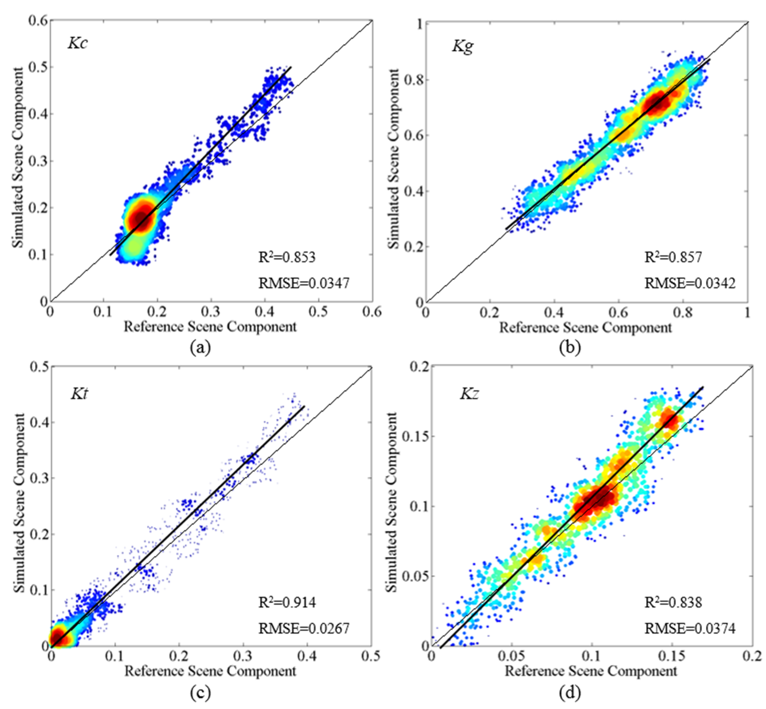
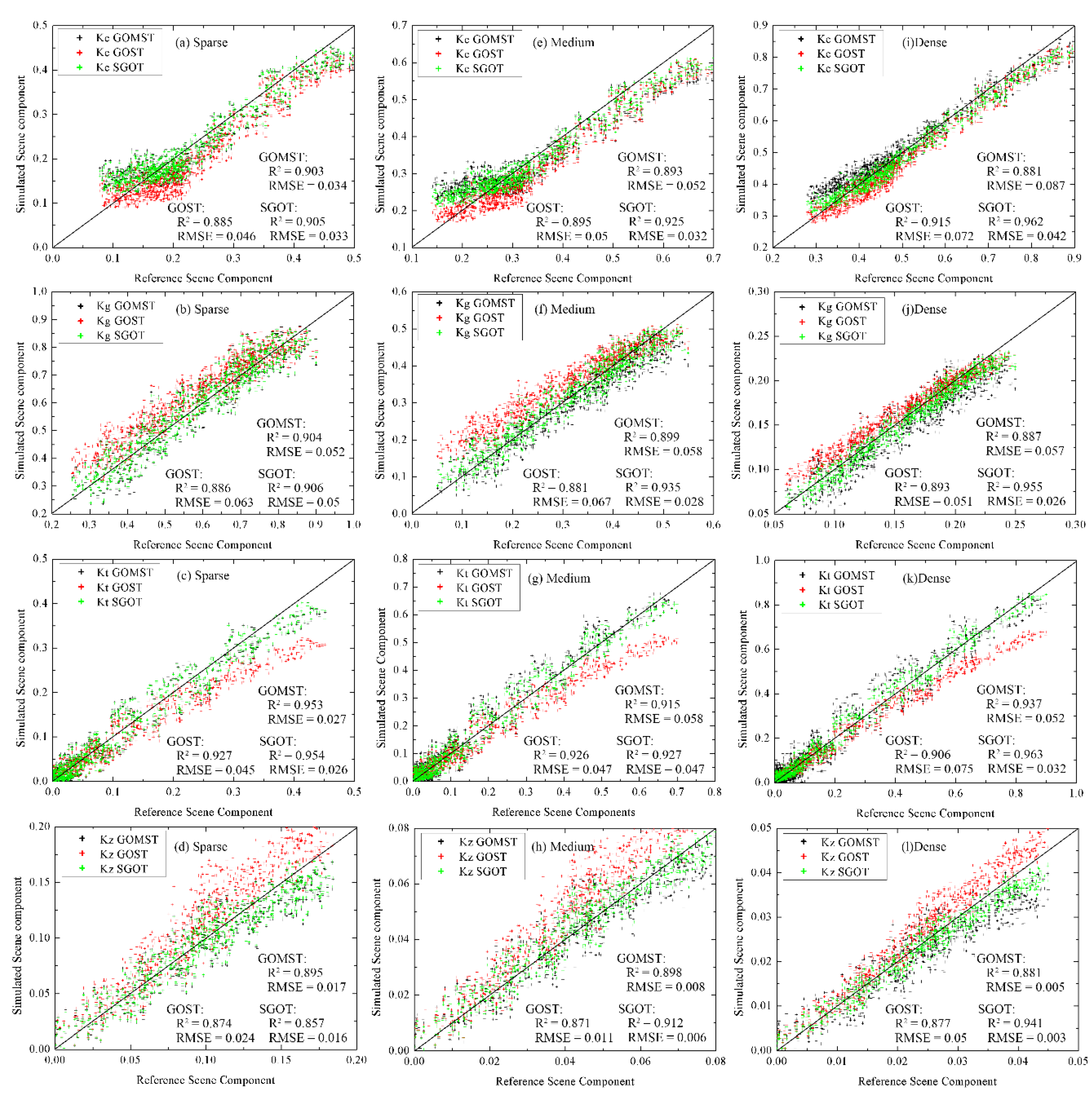
4.1. SGOT Model Validation through 3-D Virtual Canopy Model Simulations

In this section, the POV-Ray was used to generate reference scene components for validating the SGOT model. Density scatterplots between the scene components simulated by the SGOT model and generated by POV-Ray are shown in Figure 4. The scene components over different sloping surfaces and different view directions (see Table 1) were considered in this comparison. The results from the quantitative comparison show that each scene component simulated by POV-Ray and SGOT model has high consistency. The SGOT simulated scene components are consistent with POV-Ray simulations, with the RMSE (R²) of Kc, Kg, Kt, and Kz being 0.0347 (0.853), 0.0342 (0.857), 0.0267 (0.914), and 0.0374 (0.838), respectively. However, Figure 4d also shows that Kz is slightly overestimated in the high-value region, where the view azimuth is near the nadir. This may cause the upper part of the crowns to exceed the edge of the observable background. In general, the scene components simulated by the SGOT model basically coincide with the POV-Ray simulations over different surfaces and view directions, which indicates that the SGOT model has the ability to accurately simulate the scene components over sloping surfaces.

As illustrated in Figure 5, the similar distribution patterns can be figured out between the SGOT model simulated scene components (Figure 5a,c,e,g) and the POV-Ray simulated scene components (Figure 5b,d,f,h) in the principal plane. The results show that the SGOT and POV-Ray results have good consistency over different sloping surfaces. It indicates that the SGOT model has the ability to separate the scene components from sloping forest scenes. In addition, by comparing the scene components of different slopes in the same view direction, when the view direction is at the nadir in the down-slope direction, the relative differences of Kc between horizontal and sloping surfaces can reach up to 51.7% (Figure 5a,b); when the view zenith angle is 0°, the differences of Kg between horizontal and sloping surfaces can reach up to 29.3% (Figure 5c,d). Therefore, neglecting the effects of topography in GO-like models can lead to significant errors in the scene components simulation, and errors can consequently pass to canopy reflectance modeling.

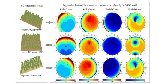
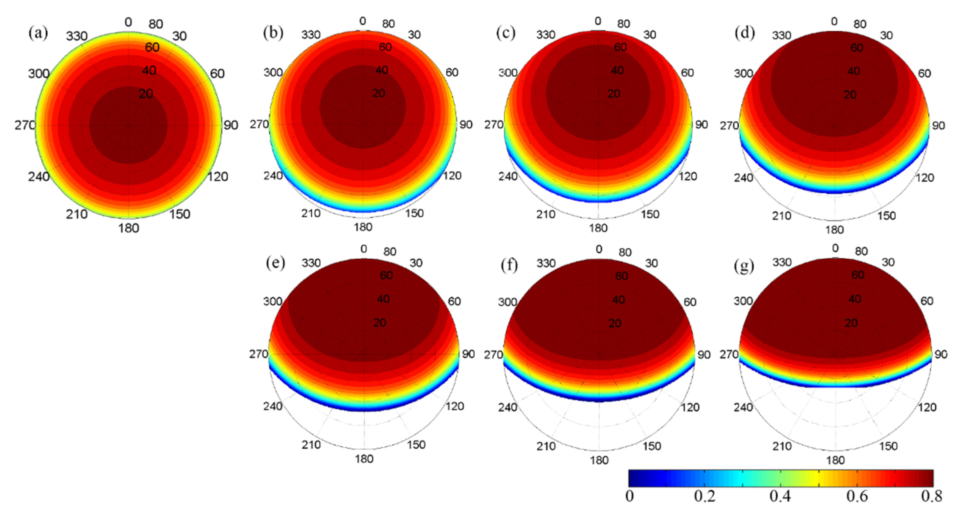
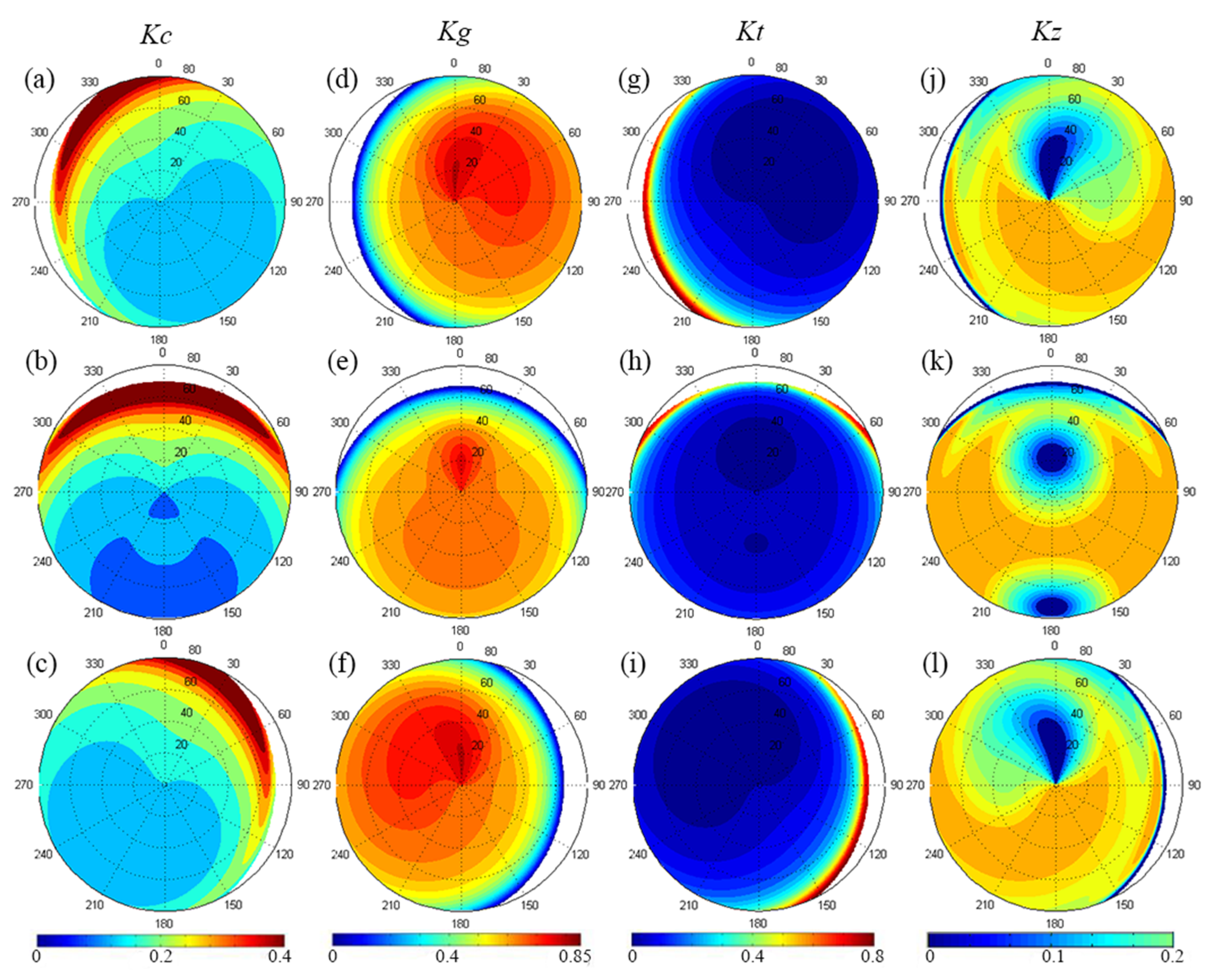
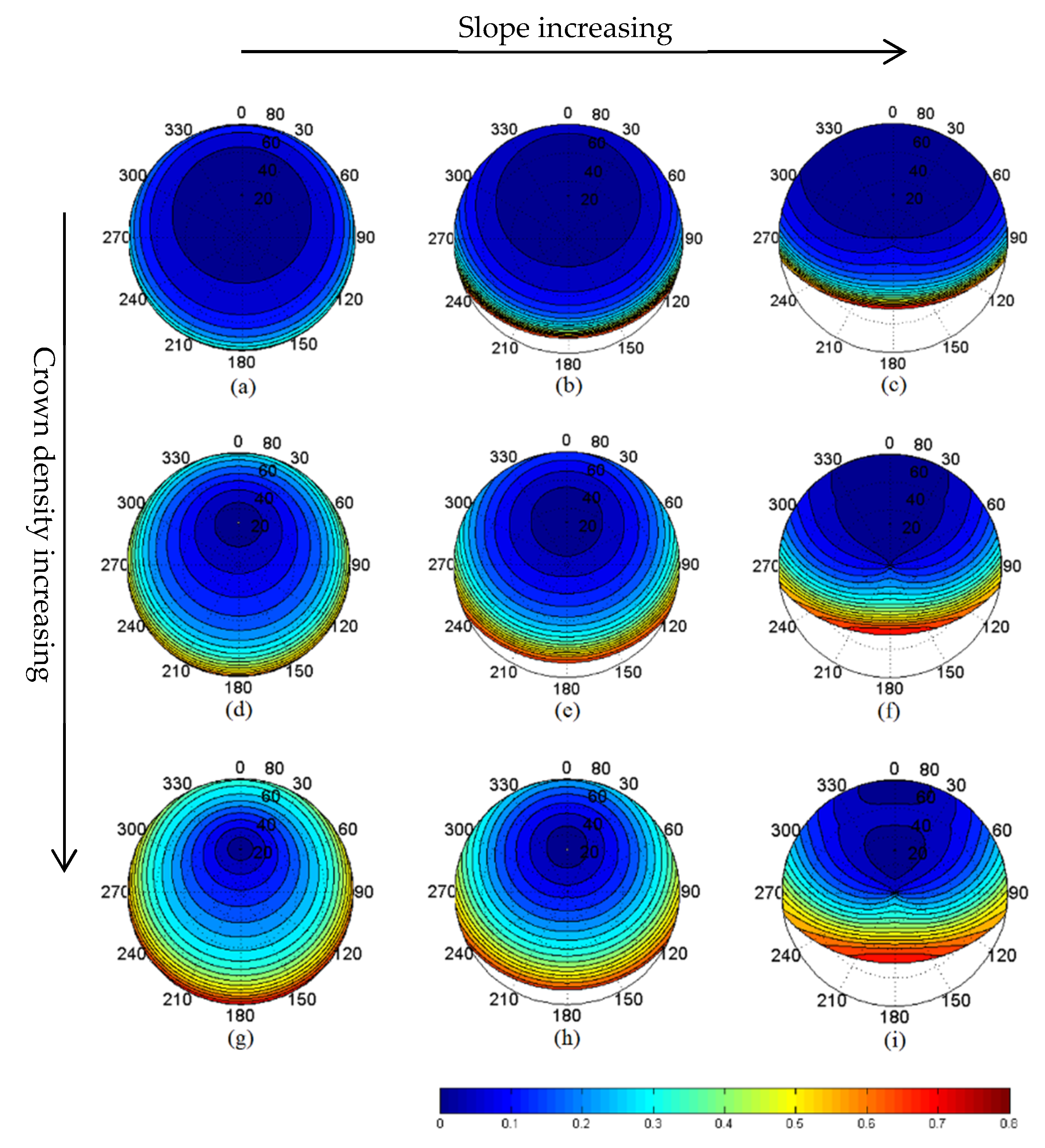
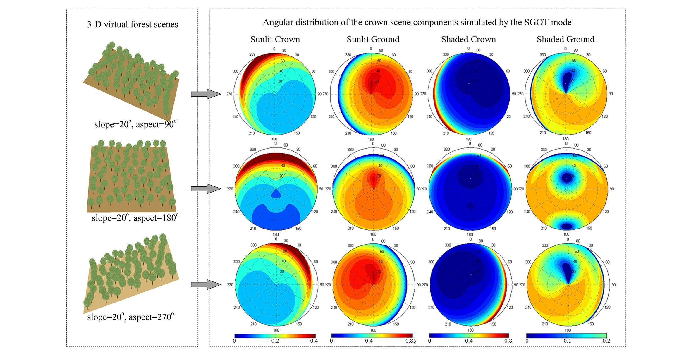
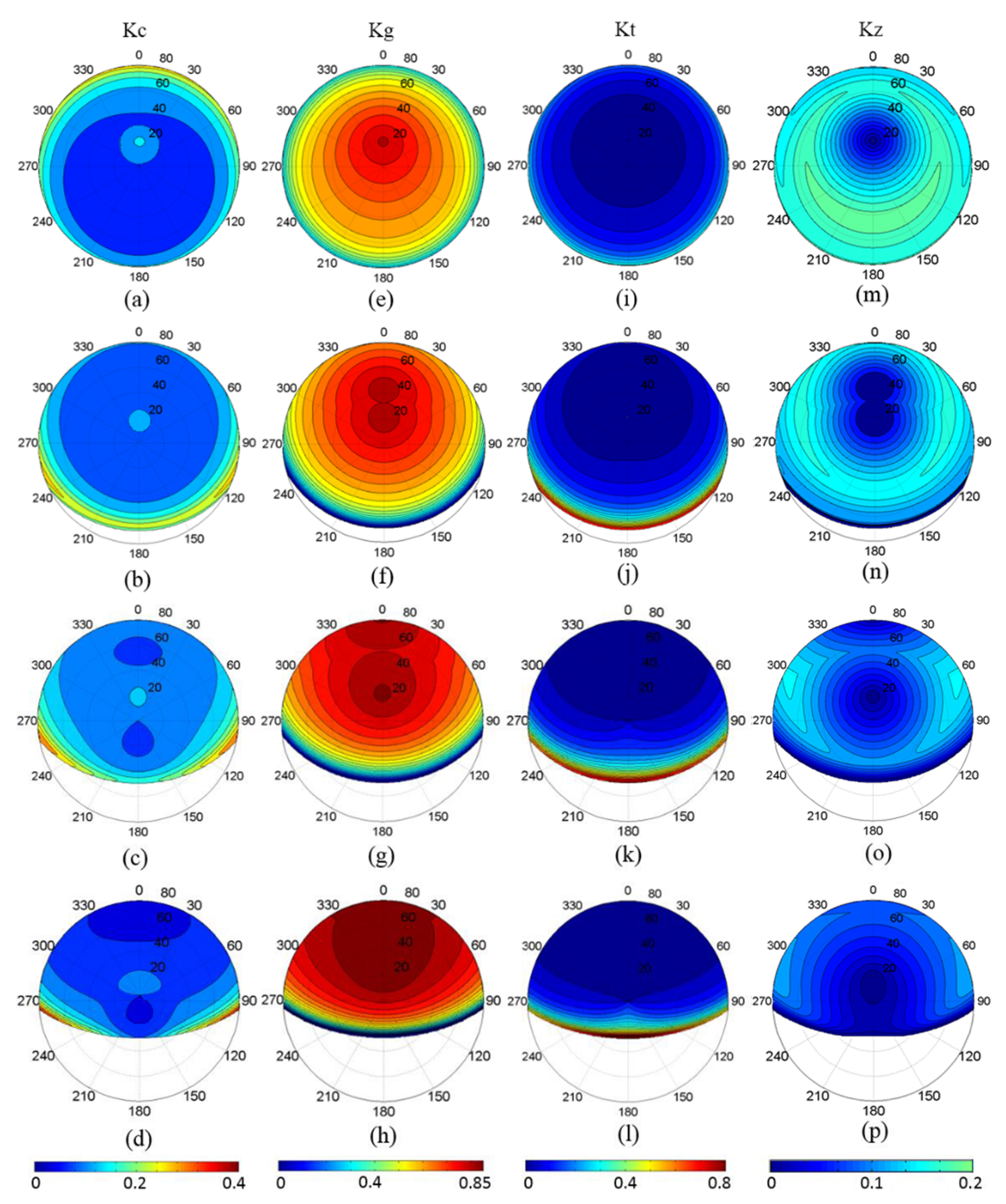
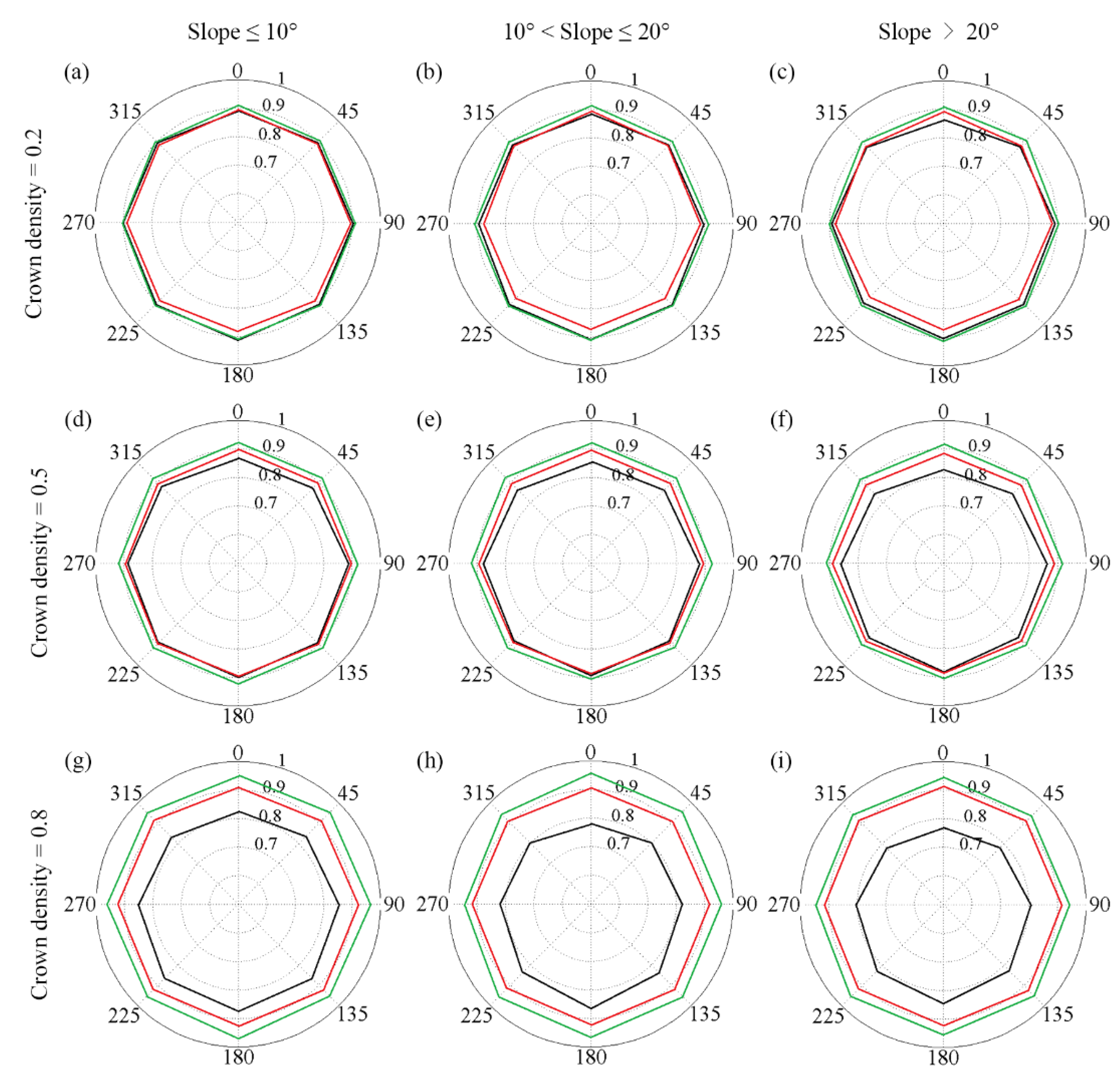
4.2. Analysis of Topographic Effects on Scene Components by SGOT Modeling

To investigate the topographic effects on scene components simulation, the scene components over surfaces with different slopes and aspects were simulated using the SGOT model. The hotspot is an important phenomenon that can be used for retrieving canopy structural parameters [40]. In this experiment, the solar zenith angle is set to 20°; when the view zenith angle is equal to the solar zenith angle, the hotspot occurs (see Figure 5). The SGOT model can successfully capture the significant increases in the simulations of scene components at the hotspot direction. The sunlit crown and background reach the peak and the shaded crown and background are 0% at the hotspot because the shaded scene components cannot be observed. The sum of the gap fraction between crowns and within crowns increases with the increase of slope; therefore, the sunlit background increases and the sunlit crown decreases in the hotspot direction (Figure 5a,c).

The lines in Figure 5a,c,e,g are smoother than those in Figure 5b,d,f,h; these slight differences may be caused by the image information extraction of POV-Ray. The setting of observation conditions (such as image resolution and camera height) in POV-Ray can affect the accuracy of image segmentation, and then affect the scene component results. Despite the lines of POV-Ray results being unsmooth, the scene components simulated by the SGOT model are very close to the POV-Ray results, and this indicates that SGOT is reliable for simulating the scene components over sloping terrain.

The gap fraction is a critical variable that can affect the scene components. Figure 6 shows the angular distributions of gap fraction in view directions over different sloping surfaces; the input parameters are the same as those in Figure 5. With the slope increasing, the gap fraction increases in the down-slope direction and decreases in the up-slope direction. Therefore, the probability of observing the background increases with the increases of slope in the down-slope direction, corresponding to the variations of Kg and Kz when the view zenith angle ranges from 20° to 80° in Figure 5c,g. Similarly, the probability of observing the crown increases with the increases of slope in the up-slope direction, corresponding to the variations of Kc and Kt when the view zenith angle ranges from −80° to 20° in Figure 5a,e.

To explore the scene component angular distributions over different terrain conditions, we simulated the scene components over different slopes and aspects based on the SGOT model, as shown in Figure 7 and Figure 8, respectively.

As illustrated in Figure 7, the first to the fourth columns represent the Kc, Kg, Kt, and Kz, respectively. The first to fourth lines represent that the slope is 0°, 20°, 40°, and 60°, respectively. The polar path represents view zenith angle, and the polar angle represents view azimuth angle. Especially when the view zenith angle is greater than (π/2)-arctan(-tanαcos(φ_v-φ_α)) along the up-slope direction, and the sensor cannot observe the target sloping surface, the topographic mask appears. Considering that the relative azimuth angle between the sun and the sloping surface is 0°, the results show that the scene components exhibit bilateral symmetry along the view principle plane over both the horizontal and sloping surfaces. Comparing the scene component distributions over the different sloping surfaces, with the slope becoming steeper, the distortion of scene components images becomes serious along the vertical plane.

As shown in Figure 7b–d, in the up-slope direction, the magnitudes of Kc distributed on both sides of the vertical plane are larger than those distributed in the middle. According to the variations of Kt in Figure 5e, because the azimuth of the sun and the viewer is opposite, the probability of observing the shaded crown increases at the nadir view direction along the view principal plane. Therefore, as the relative azimuth angle between the viewer and the sloping surface decreases from 180°, the probability of observing the sunlit middle and lower parts of the crown increases gradually.

Figure 8 shows how the scene component changes with the aspect ranging from 90° to 270° in 90° intervals. Comparing the scene components over the sloping surfaces with aspects of 90° (Figure 8a,d,g,j) and 270° (Figure 8c,f,i,l), their distributions are completely symmetrical. However, there are some obvious differences between the distributions of scene components with aspects of 0° (Figure 7a,e,i,m) and 180° (Figure 8b,e,h,k). Different aspects alter the gap fraction in the solar direction, resulting in the increase of the sunlit area when the relative azimuth angle between the sun and the sloping surface is less than 90°, or the decrease of the sunlit area when the relative azimuth angle between the sun and the sloping surface is more than 90°. Therefore, when the sloping surface faces the sun, Kt and Kz decrease in the direction close to the sun (see Figure 7j,n) because the shadow area observed in the direction near the sun is less than that of 180° in Figure 8h,k; meanwhile, the distributions of Kc (Figure 7b and Figure 8b) and Kg (Figure 7f and Figure 8e) show the opposite characteristics to Kt and Kz. To reveal the effects of slopes and aspects, the experiments show that the different slope and relative azimuth angles among the sun, the viewer, and the slope can cause significant changes in scene components. The SGOT model shows good mechanism performance in the estimations of scene components and can accurately capture the variations of scene components under different illumination, observation, and terrain conditions.

In addition, as shown in Figure 9, the scene components of Kt over sloping surfaces with different crown density were also compared. The results show that crown density is another important factor affecting scene components, except for terrain factors. Different from the sparse forest (the first row in Figure 9), with the increase of crown density (see from row 2 to row 3 in Figure 9), the contours are more densely distributed in the up-slope direction and more dispersed in the down-slope direction. The higher crown density means the gap size between crowns becomes smaller, the probability of observing the crowns increased and that of the background decreased, respectively. Especially when the view direction is far from the solar direction, the magnitude of Kt increases significantly with the increase of crown density. With the increase of slope, Kt shows similar trends in the three vegetation coverage areas.

To summarize, the above analysis of GOST simulations shows that the main factors affecting the scene components over sloping surfaces include slope, aspect, and crown density. Among them, the slope and the crown density can alter the magnitude of scene components by adjusting the gap fraction, while the aspect can affect the distribution pattern of scene components by altering the relative azimuth angle among the sun, the viewer, and the sloping surface.

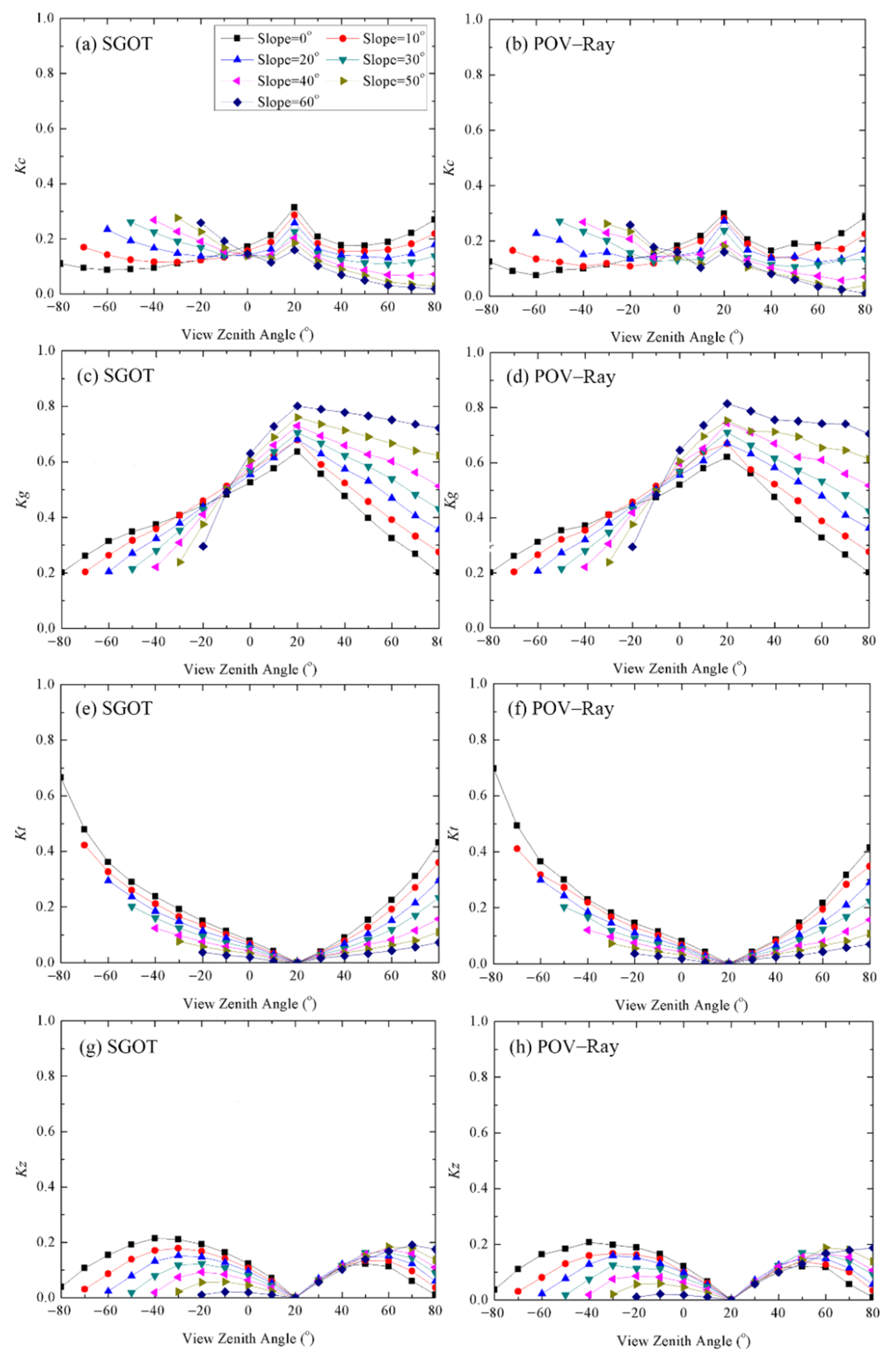
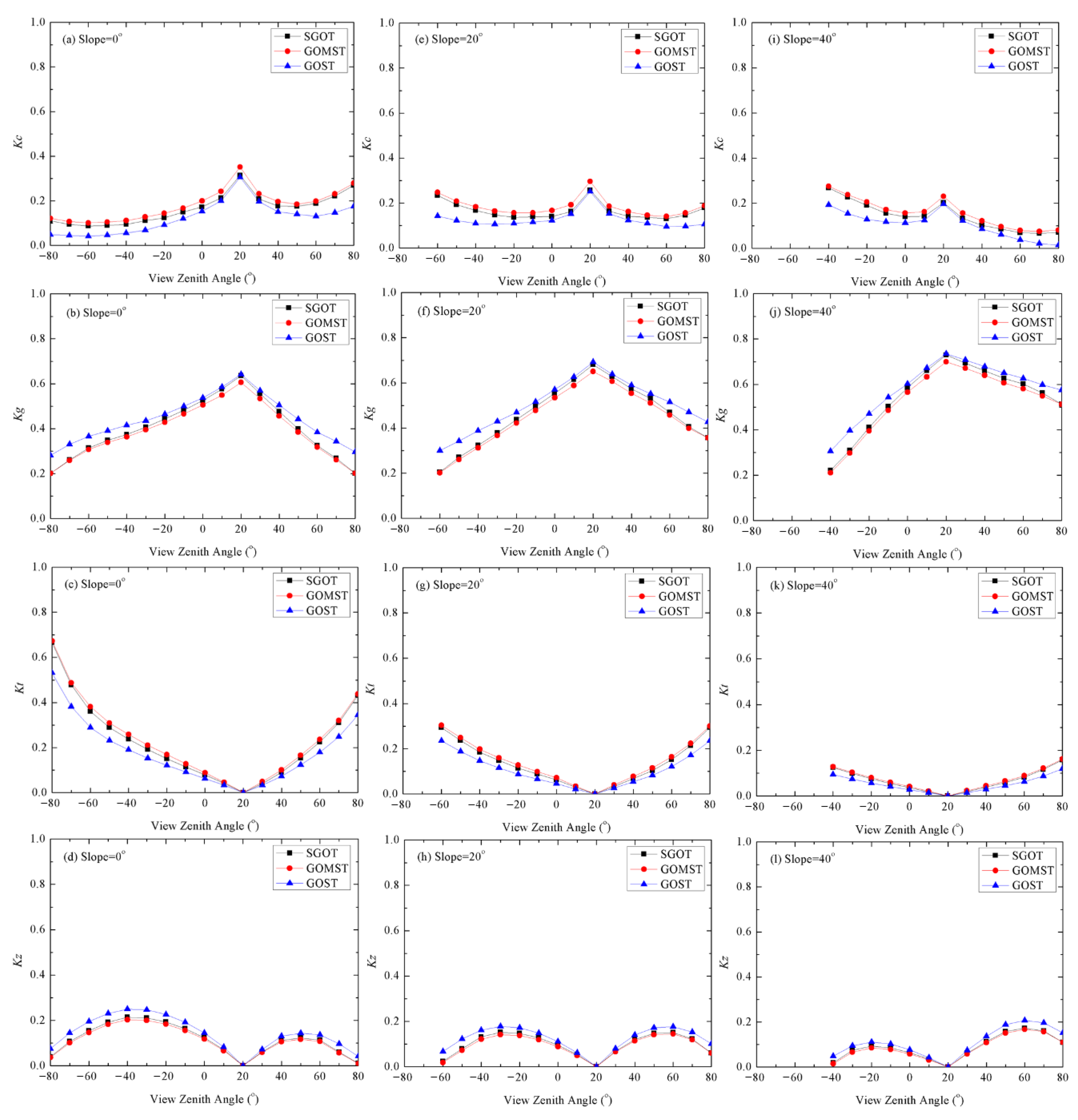
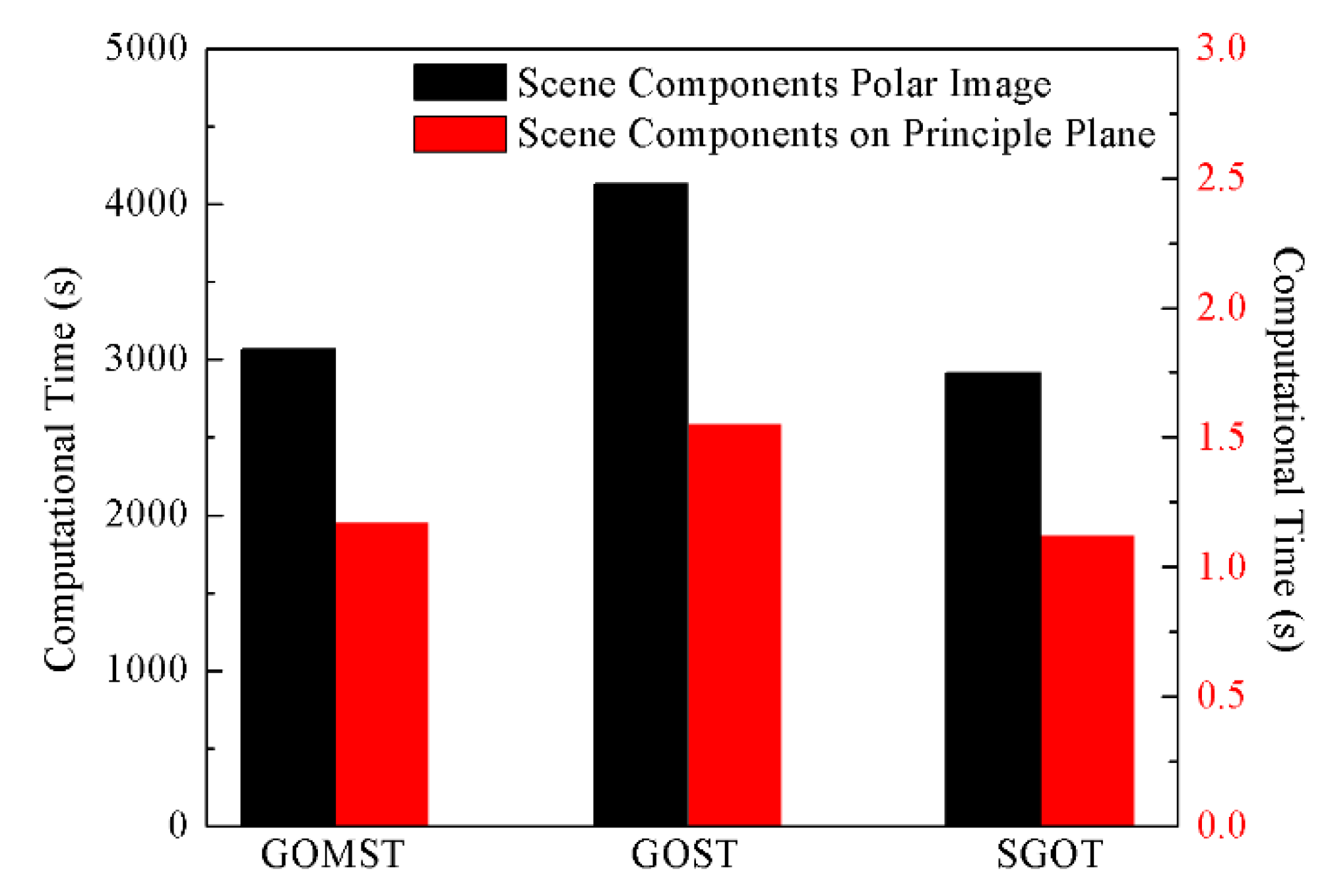
4.3. Comparison with Typical GO-Like Models

As shown in Figure 10, the scene component simulations of SGOT model and GOMST model have good consistency, just with a slight difference on different surfaces. Considering the formulation of the gap fraction within crowns, the area of background observed in SGOT scenes is larger than that of GOMST scenes. Therefore, Kg and Kz simulated by GOMST are slightly higher than SGOT simulations, and the difference between GOMST and SGOT reaches the maximum at the hotspot. Similarly, Kc and Kt simulated by GOMST are slightly lower than SGOT simulations.

However, there are systematic differences between the simulations of the SGOT model and the GOST model. Figure 10 also shows that the scene components from crowns (Kc and Kt) simulated by SGOT are higher than the GOST simulations. In addition, the scene components from background (Kg and Kz) simulated by SGOT are lower than the GOST simulations as shown in Figure 10b,d,f,h,j,l. These comparison results indicate that more sunlight can reach the background through the crowns in GOST simulation than in SGOT and GOMST. By comparing the tree distribution patterns in two models, the Neyman type-A distribution [41] and the Poisson distribution were assumed in the GOST model and the random distribution was assumed in the SGOT model and the GOMST model. The different tree distribution patterns can affect the projected area of the background in the solar and view directions, and the difference between the SGOT and GOST simulations increases with the increase of view zenith angle, because of the larger number of overlapping crowns. Therefore, there is a certain gap between the magnitude of scene component simulations of the SGOT model and the GOST model.

In addition, compared with the GOMST model, the SGOT model takes the gap fraction within canopies into account. The gap fraction within canopies has different effects on the results in the areas with different crown density. Therefore, the scene component simulations between the SGOT model and the GOMST model in the higher crown density area may be quite different. Figure 11 shows the scatterplots between simulated scene components from the different models with spare, medium, and dense crown densities, which were set as 0.2, 0.5, and 0.8, respectively. For the spare crown density forest scenes (Figure 11a–d), the gap fraction within crowns accounts for a small proportion in the whole scene; the simulation accuracy of the SGOT model is almost the same as that of the GOMST model. However, with the increase of crown density, the difference between the simulation results of the GOMST model and the SGOT model increases gradually. For the medium and dense crown density forest scenes, Figure 11e–l, the dots in the plots simulated by the SGOT model are more close to the POV-Ray simulations. The higher the vegetation coverage, the greater the accuracy improvement of SGOT shows. The differences of RMSE (R²) for Kc, Kg, Kt, and Kz between the SGOT model and the GOMST model simulations for dense crown density are −0.045 (0.081), −0.031 (0.068), −0.02 (0.026), and −0.002 (0.06), respectively. With respect to the GOST simulations, there are systematic differences between the results of the SGOT model and the GOST model. As shown in Figure 11a,c,e,g,i,k, the scene components of crown simulated by the GOST model are underestimated, and as shown in Figure 11b,d,f,h,j,l, the scene components of background simulated by the GOST model are overestimated, which may also be caused by the different tree distribution patterns assumed in SGOT and GOST. Therefore, different endogenous mechanisms of the compared models lead to different results, as mentioned in Figure 11; with the increase of view zenith angle, the probability of observing the background in the GOST scene is higher than that in the SGOT and GOMST scenes. It can be concluded that the simulation accuracy of the SGOT model is better than that of the GOST model when the distribution of forest stand is random. Therefore, the SGOT model appears to have better performance in scene component simulation, especially in areas with high crown density.

Considering the difference in internal mechanism of each model, different view directions, slopes, and crown densities may have different effects on the results. To figure out the influence of each factor, the simulation accuracy of each model in different view azimuths (the interval of the azimuth was set to 45°) and various crown densities (the same as the settings in Figure 11) over the slight (<10°), moderate (10–20°), and steep (>20°) sloping surfaces (the aspect was set to 0°) was compared in this section. Figure 12 shows the correlation between the simulated sunlit crown of different models and POV-Ray results; the correlation coefficients of the SGOT, GOMST, and GOST simulations were represented by the green, black, and red lines, respectively; the closer the line is to the outermost circle, the better the simulation result of the model. With the slope increasing, the gap between the correlation coefficients of SGOT and GOMST results is gradually increasing, especially when the view azimuth is close to 0°, because there are fewer crowns overlapped in the direction of sight in the down-slope direction, and the gap fraction within crowns has a significant effect on the results. As shown in Figure 12c,f,i, with the increase of crown density, the improvement of SGOT becomes more obvious. This comparison indicates that SGOT can adapt to a larger range of view azimuth, slope, and crown density.

With respect to the computational efficiency of each model, as shown in Figure 13, in this experiment, the computational efficiency of the SGOT model is slightly better than the GOMST model and is obviously better than that of the GOST model. The timer recording shows that it requires 29.5% less time to run the SGOT model than the GOST model and 4% less time than the GOMST model for scene component simulations.

Compared with the GOST model, the SGOT model ignored the 3-D complex internal structure of the crowns; the distribution of leaves in the crown was not considered in SGOT. Therefore, the calculation of gap fraction in SGOT was simpler than that in the GOST model, which greatly reduced the computational time. It can be speculated that considerable time can also be saved in the subsequent canopy reflectance calculation.

5. Discussion

Crown scene components play an important role in canopy reflectance modeling, but topography affects the fraction of scene components of the canopy and background, resulting in the observed reflectance distortion. For correcting this distortion, the existing models greatly increased the mathematical complexity while improving description of terrain and crown structure, which dramatically decreased the computational efficiency so as to limit their universal applications. In this paper, we developed a simplified geometric-optical model (SGOT) to simulate crown scene components over sloping terrain and investigated the effects of topographic factors on scene components. To achieve these goals, we presented an extension of the GOMST model, mainly focusing on two aspects in scene components modeling. First, a new projection relationship between the vertically projected area on a horizontal surface and a sloping surface projected area is proposed to make the projection conversion process more convenient and this can retain the geotropism of tree growth. Second, the study gives a detailed account of a simplified scheme for the internal structure of the tree crown to make the SGOT model more physically sound and computationally efficient.

However, the crown shape was assumed to be ellipsoid in this study; this hypothesis refers to the GOMST model to facilitate comparison between models. Previous studies have shown that the crown shape has significant effects on the simulation of scene components [42]; the crown projection area in different planes and the volume of the crown need to be adjusted according to other specific shapes [17]. As mentioned above, the projected area of the tree crown can be derived from the vertically projected area and the shape-adjusting factor; the SGOT model has the ability to simulate the scene components of tree crowns with different shapes (for details, please see Appendix A). Additionally, the crown was assumed to be uniformly filled with leaves in the proposed model; this assumption referred to extending ROSS [3] to sloping surfaces by Combal et al. [27]. In fact, the leaves are not uniformly and randomly distributed within crowns [10,17,23], e.g., in conifer stands, needles are grouped into shoots, branches, and whorls; all these substructures within crowns have a significant effect on the bidirectional reflectance properties [10]. However, the complex internal structure of tree crowns should increase the computational complexity of implementing the model [43]. Simultaneously, the existing study reported that the woody elements are negligible in the upper canopy in a dense young forest stand [44], but the radiance contributions from the trunk concentrated in the lower part of the canopy cannot be ignored [44,45]; in particular, the difference in the area fraction of the trunk observed around noon is very obvious [46]. The tree trunks also play a significant role in calculating and even redefining the crown scene components. The incorporation of a parameterization-simple method of scene component simulation for the canopy reflectance model can improve the computational efficiency [29]; therefore, the internal structure of the tree crown was simplified in the SGOT model. In practice, we need to discover an appropriate balance between accuracy and practicability of the model according to the real structure of vegetation. In addition, it should be noted that SGOT can be used for simulating crown scene components on slopes at canopy scale. However, in a real scene with large spatial scale and coarse spatial resolution, the effects of local crown dimensions and topography on crown scene component simulation become weaker due to smooth overall crown parameters, slope, and aspect [27]; thus, the solar and view directions, the vegetation coverage, and LAI become the main factors affecting the simulation results. In contrast, the effects of crown dimensions and topographic at the small spatial scale and finer spatial resolution are significant [47,48]. Specifically, the canopy scale level terrains affect the distribution of solar radiance and the scattering contribution items in view directions are affected by the distribution of crown shadow and terrain masking [49].

In model comparisons, we compared the view-geometric-induced scene component variations over different sloping surfaces. In fact, setting multiple solar zenith angles and azimuth angles can significantly affect crown projection and further affect the crown scene components simulation [50], but the main content of this study is intended to reveal the influence of topography on scene components, while the influence of solar direction was not discussed in this work. In addition, we compared the accuracy of SGOT with GOMST and GOST models in the same virtual forest scenes; the SGOT model has been proven to perform well in crown scene components simulation under various terrain conditions and crown densities. The random tree distribution pattern assumed in GOMST and SGOT is consistent with that set in the virtual forest scenes, but the nonrandom Neyman type-A distribution [41] was assumed in GOST, in which the mathematical description of the crown structure is more similar to the real tree crown, especially for sparse forests [28]. Therefore, the SGOT simulations can be considered more suitable for the forest with randomly distributed tree crowns. Further comparison of the model performances in the real mountainous forest scene is still essential.

Existing studies on canopy reflectance modeling and biophysical parameter retrieval for mountainous regions mostly used canopy reflectance models that were developed for flat surfaces [19,20] through accounting for the terrain effect by converting the solar-view geometry from a flat surface to the local terrain. Such treatment neglected the modulation of topography on canopy structure [17,51], inducing large uncertainties in biophysical parameter retrieval [52]. SGOT will facilitate forward canopy reflectance modeling and biophysical parameter retrieval in mountainous regions because it can transform the areal proportion of scattering contributions from a flat surface to a sloping surface accurately and efficiently with identical biophysical parameters. In addition, because the solar-view geometry was explicitly involved in SGOT, multi-angle data can be readily exploited to improve the ability of biophysical parameter retrieval [53]. Thus, the strategy of incorporating SGOT into a canopy reflectance model can improve the model performance without violating the terrain-induced adjustment of canopy structure.

6. Conclusions

In this paper, we proposed a simplified geometric-optical model to simulate crown scene components over rugged terrain (SGOT). To verify the performance of the SGOT model, the computer 3-D virtual model POV-Ray and GO-like models (GOMST and GOST) were used for comparison. The results showed that the SGOT model can accurately simulate the scene components over different sloping surfaces (R² for the areal proportions of sunlit crown (Kc), sunlit background (Kg), shaded crown (Kt), and shaded background (Kz) are 0.853, 0.857, 0.914, and 0.838, with RMSE of 0.0347, 0.0342, 0.0267, and 0.0374, respectively) and reproduce the topographic effects on the simulations of scene components well. Compared with the GOMST model, the SGOT model has higher simulation accuracy in the forests, especially with dense crown density. In addition, the computational time of the SGOT model is 29.5% faster than the GOST model; the efficiency of the SGOT model has been significantly improved. This contribution demonstrated that the SGOT model can improve simulation accuracy and computational efficiency in scene components modeling over rugged terrain. It can help us to understand the topographic effects on scattered components and improve the performance of the radiation contributions calculation, and also provide an efficient and reliable tool for upscaling the reflectance of canopy components to the canopy. The projection method and the simplified scheme of tree crown proposed in SGOT will be expected to be a paradigm to extend and improve the performance of the existing canopy reflectance models. Further improvements to the SGOT model would include a more applicable projection algorithm, accounting for tree trunk effects, and exploration of the potential of the SGOT model to improve the performance of canopy reflectance models.

References

1. Verrelst, J.; Camps-Valls, G.; Muñoz-Marí, J.; Rivera, J.P.; Veroustraete, F.; Clevers, J.G.P.W.; Moreno, J. Optical remote sensing and the retrieval of terrestrial vegetation bio-geophysical properties—A review. ISPRS J. Photogramm. Remote Sens. 2015, 108, 273–290. [Google Scholar] [CrossRef]
2. Verhoef, W. Light scattering by leaf layers with application to canopy reflectance modeling: The SAIL model. Remote Sens. Environ. 1984, 16, 125–141. [Google Scholar] [CrossRef] [Green Version]
3. Ross, J. The radiation regime and architecture of plant stands. J. Ecol. 1981, 71, 344. [Google Scholar] [CrossRef]
4. Li, X.; Strahler, A.H. Geometric-optical modeling of a conifer forest canopy. IEEE Trans. Geosci. Remote Sens. 1985, GE-23, 705–721. [Google Scholar] [CrossRef] [Green Version]
5. Li, X.; Strahler, A.H. Geometric-optical bidirectional reflectance modeling of the discrete crown vegetation canopy: Effect of crown shape and mutual shadowing. IEEE Trans. Geosci. Remote Sens. 1992, 30, 276–292. [Google Scholar] [CrossRef]
6. Li, X.; Woodcock, C.; Davis, R. A hybrid heometric optical and radiative transfer approach for modeling pyranometer measurements under a jack pine forest. Geogr. Inf. Sci. 1995, 1, 34–40. [Google Scholar]
7. Huemmrich, K.F. The geosail model: A simple addition to the SAIL model to describe discontinuous canopy reflectance. Remote Sens. Environ. 2001, 75, 423–431. [Google Scholar] [CrossRef]
8. Gastellu-Etchegorry, J.P.; Martin, E.; Gascon, F. DART: A 3D model for simulating satellite images and studying surface radiation budget. Int. J. Remote Sens. 2004, 25, 73–96. [Google Scholar] [CrossRef]
9. Qi, J.; Xie, D.; Xu, Y.; Yan, G. Principles and applications of the 3D radiative transfer model LESS. Remote Sens. Technol. Appl. 2019, 34, 914–924. [Google Scholar] [CrossRef]
10. Chen, J.M.; Leblanc, S.G. A four-scale bidirectional reflectance model based on canopy architecture. IEEE Trans. Geosci. Remote Sens. 1997, 35, 1316–1337. [Google Scholar] [CrossRef]
11. Gu, D.; Gillespie, A. Topographic normalization of Landsat TM images of forest based on subpixel sun-canopy-sensor geometry. Remote Sens. Environ. 1998, 64, 166–175. [Google Scholar] [CrossRef]
12. Li, A.; Wang, Q.; Bian, J.; Lei, G. An improved physics-based model for topographic correction of Landsat TM images. Remote Sens. 2015, 7, 6296–6319. [Google Scholar] [CrossRef] [Green Version]
13. Soenen, S.A.; Peddle, D.R.; Coburn, C.A. SCS+C: A modified sun-canopy-sensor topographic correction in forested terrain. IEEE Trans. Geosci. Remote Sens. 2005, 43, 2148–2159. [Google Scholar] [CrossRef]
14. Yin, G.; Li, A.; Wu, S.; Fan, W.; Zeng, Y.; Kai, Y.; Xu, B.; Jing, L.; Liu, Q. Plc: A simple and semi-physical topographic correction method for vegetation canopies based on path length correction. Remote Sens. Environ. 2018, 215, 184–198. [Google Scholar] [CrossRef]
15. Proy, C.; Tanre, D.; Deschamps, P.Y. Evaluation of topographic effects in remotely sensed data. Remote Sens. Environ. 1989, 30, 21–32. [Google Scholar] [CrossRef]
16. Sandmeier, S.; Itten, K. A physically-based model to correct atmospheric and illumination effects in optical satellite data of rugged terrain. IEEE Trans. Geosci. Remote Sens. 1997, 35, 708–717. [Google Scholar] [CrossRef] [Green Version]
17. Fan, W.; Chen, J.M.; Ju, W.; Zhu, G. Gost: A geometric-optical model for sloping terrains. IEEE Trans. Geosci. Remote Sens. 2014, 52, 5469–5482. [Google Scholar] [CrossRef]
18. Yin, G.; Li, A.; Zhao, W.; Jin, H.; Bian, J.; Wu, S. Modeling canopy reflectance over sloping terrain based on path length correction. IEEE Trans. Geosci. Remote Sens. 2017, 55, 4597–4609. [Google Scholar] [CrossRef]
19. Gonsamo, A.; Chen, J.M. Improved LAI algorithm implementation to MODIS data by incorporating background, topography, and foliage clumping information. IEEE Trans. Geosci. Remote Sens. 2013, 52, 1076–1088. [Google Scholar] [CrossRef]
20. Pasolli, L.; Asam, S.; Castelli, M.; Bruzzone, L.; Wohlfahrt, G.; Zebisch, M.; Notarnicola, C. Retrieval of leaf area index in mountain grasslands in the Alps from MODIS satellite imagery. Remote Sens. Environ. 2015, 165, 159–174. [Google Scholar] [CrossRef]
21. Verhoef, W.; Bach, H. Coupled soil–leaf-canopy and atmosphere radiative transfer modeling to simulate hyperspectral multi-angular surface reflectance and TOA radiance data. Remote Sens. Environ. 2007, 109, 166–182. [Google Scholar] [CrossRef]
22. Schaaf, C.B.; Li, X.; Strahler, A.H. Topographic effects on bidirectional and hemispherical reflectances calculated with a geometric-optical canopy model. IEEE Trans. Geosci. Remote Sens. 1994, 32, 1186–1193. [Google Scholar] [CrossRef]
23. Fan, W.; Li, J.; Liu, Q. Gost2: The improvement of the canopy reflectance model gost in separating the sunlit and shaded leaves. IEEE J. Sel. Top. Appl. Earth Observ. Remote Sens. 2015, 8, 1423–1431. [Google Scholar] [CrossRef]
24. Disney, M.; Lewis, P.; North, P.R.J. Monte carlo ray tracing in optical canopy reflectance modelling. Int. J. Remote Sens. 2000, 18, 163–196. [Google Scholar] [CrossRef]
25. Omari, K.; White, H.P.; Staenz, K. Multiple scattering within the flair model incorporating the photon recollision probability approach. Geosci. Remote Sens. IEEE Trans. 2009, 47, 2931–2941. [Google Scholar] [CrossRef]
26. Wu, S.; Wen, J.; Lin, X.; Hao, D.; You, D.; Xiao, Q.; Liu, Q.; Yin, T. Modeling discrete forest anisotropic reflectance over a sloped surface with an extended GOMS and SAIL model. IEEE Trans. Geosci. Remote Sens. 2019, 57, 944–957. [Google Scholar] [CrossRef]
27. Combal, B.; Isaka, H.; Trotter, C. Extending a turbid medium BRDF model to allow sloping terrain with a vertical plant stand. IEEE Trans. Geosci. Remote Sens. 2000, 38, 798–810. [Google Scholar] [CrossRef]
28. Geng, J.; Chen, J.; Fan, W.; Tu, L.; Tian, Q.; Yang, R.; Yang, Y.; Wang, L.; Lv, C.; Wu, S. Gofp: A geometric-optical model for forest plantations. IEEE Trans. Geosci. Remote Sens. 2017, 55, 5230–5241. [Google Scholar] [CrossRef]
29. Yin, G.; Li, J.; Liu, Q.; Fan, W.; Xu, B.; Zeng, Y.; Zhao, J. Regional leaf area index retrieval based on remote sensing: The role of radiative transfer model selection. Remote Sens. 2015, 7, 4604–4625. [Google Scholar] [CrossRef] [Green Version]
30. Li, X.; Strahler, A. Mutual shadowing and directional reflectance of a rough surface—A geometric-optical model. In Proceedings of the 12th Annual International Geoscience and Remote Sensing Symposium, Houston, TX, USA, 26–29 May 1992; Volume 1, pp. 766–768. [Google Scholar]
31. Montes, F.; Pita, P.; Rubio, A.; Cañellas, I. Leaf area index estimation in mountain even-aged Pinus silvestris L. Stands from hemispherical photographs. Conf. Agric. For. Meteorol. 2007, 145, 215–228. [Google Scholar] [CrossRef]
32. Alijafar, M.; Wout, V.; Massimo, M.; Ben, G. Modeling top of atmosphere radiance over heterogeneous non-lambertian rugged terrain. Remote Sens. 2015, 7, 8019–8044. [Google Scholar] [CrossRef] [Green Version]
33. Norman, J.M.; Welles, J.M. Radiative transfer in an array of canopies. Agron. J. 1983, 75, 481–488. [Google Scholar] [CrossRef]
34. Strahler, A.H.; Jupp, D.L.B. Modeling bidirectional reflectance of forests and woodlands using boolean models and geometric optics. Remote Sens. Environ. 1990, 34, 153–166. [Google Scholar] [CrossRef]
35. Sinoquet, H.; Thanisawanyangkura, S.; Mabrouk, H.; Kasemsap, P. Characterization of the light environment in canopies using 3D digitising and image processing. Ann. Bot. 1998, 82, 203–212. [Google Scholar] [CrossRef] [Green Version]
36. Kuusk, A. The Hot Spot Effect in Plant Canopy Reflectance; Springer: Berlin/Heidelberg, Germany, 1991; pp. 139–159. [Google Scholar]
37. Wang, J.; Feng, Z.; Hu, L.I.; Tao, Y.U.; Xingfa, G.U.; Lian, X. Sunlit coponents’ fractions and gap fraction of canopies based on POV-ray. Remote Sens. 2010, 14, 232–251. [Google Scholar] [CrossRef]
38. Shang, H.; Zhao, F.; Zhao, H. The analysis of errors for field experiment based on POV-ray. In Proceedings of the Geoscience and Remote Sensing Symposium, Munich, Germany, 22–27 July 2012; pp. 4805–4808. [Google Scholar]
39. Casa, R.; Jones, H.G. LAI retrieval from multiangular image classification and inversion of a ray tracing model. Remote Sens. Environ. 2005, 98, 414–428. [Google Scholar] [CrossRef]
40. Simic, A.; Chen, J.M.; Freemantle, J.R.; Miller, J.R.; Pisek, J. Improving clumping and LAI algorithms based on multiangle airborne imagery and ground measurements. IEEE Trans. Geosci. Remote Sens. 2010, 48, 1742–1759. [Google Scholar] [CrossRef]
41. Neyman, J. On a new class of contagious distributions, applicable in entomology and bacteriology. Ann. Math. Stat. 1939, 10, 35–57. [Google Scholar] [CrossRef]
42. Rautiainen, M.; Stenberg, P.; Nilson, T.; Kuusk, A. The effect of crown shape on the reflectance of coniferous stands. Remote Sens. Environ. 2004, 89, 41–52. [Google Scholar] [CrossRef]
43. Zeng, Y.; Li, J.; Liu, Q.; Huete, A.; Yin, G.; Xu, B.; Fan, W.; Zhao, J.; Yan, K.; Mu, X. A radiative transfer model for heterogeneous agro-forestry scenarios. IEEE Trans. Geosci. Remote Sens. 2016, 54, 4613–4628. [Google Scholar] [CrossRef]
44. Verrelst, J.; Schaepman, M.E.; Malenovský, Z.; Clevers, J.G.P.W. Effects of woody elements on simulated canopy reflectance: Implications for forest chlorophyll content retrieval. Remote Sens. Environ. 2010, 114, 647–656. [Google Scholar] [CrossRef] [Green Version]
45. Asner, G. Biophysical and biochemical sources of variability in canopy reflectance. Remote Sens. Environ. 1998, 64, 234–253. [Google Scholar] [CrossRef]
46. Tian, S.; Zheng, G.; Eitel, J.; Zhang, Q. A lidar-based 3-D photosynthetically active radiation model reveals the spatiotemporal variations of forest sunlit and shaded leaves. Remote Sens. 2021, 13, 1002. [Google Scholar] [CrossRef]
47. Wen, J.; Liu, Q.; Liu, Q.; Xiao, Q.; Li, X. Scale effect and scale correction of land-surface albedo in rugged terrain. Int. J. Remote Sens. Int. J. Remote Sens. 2009, 30, 5397–5420. [Google Scholar] [CrossRef]
48. Roupioz, L.; Nerry, F.; Jia, L.; Menenti, M. Improved surface reflectance from remote sensing data with sub-pixel topographic information. Remote Sens. 2014, 6, 10356–10374. [Google Scholar] [CrossRef] [Green Version]
49. Wen, J.; Liu, Q.; Xiao, Q.; Liu, Q.; You, D.; Hao, D.; Wu, S.; Lin, X. Characterizing land surface anisotropic reflectance over rugged terrain: A review of concepts and recent developments. Remote Sens. 2018, 10, 370. [Google Scholar] [CrossRef] [Green Version]
50. Cheng, J.; Wen, J.; Xiao, Q.; Wu, S.; Hao, D.; Liu, Q. Extending the GOSAILT model to simulate sparse woodland bi-directional reflectance with soil reflectance anisotropy consideration. Remote Sens. 2022, 14, 1001. [Google Scholar] [CrossRef]
51. Fan, W.; Chen, J.M.; Ju, W.; Nesbitt, N. Hybrid geometric optical–radiative transfer model suitable for forests on slopes. IEEE Trans. Geosci. Remote Sens. 2014, 52, 5579–5586. [Google Scholar] [CrossRef]
52. Soenen, S.; Peddle, D.; Hall, R.J.; Coburn, C.; Hall, F. Estimating aboveground forest biomass from canopy reflectance model inversion in mountainous terrain. Remote Sens. Environ. 2010, 114, 1325–1337. [Google Scholar] [CrossRef]
53. Chen, J.M.; Liu, J.; Leblanc, S.G.; Lacaze, R.; Roujean, J.-L. Multi-angular optical remote sensing for assessing vegetation structure and carbon absorption. Remote Sens. Environ. 2003, 84, 516–525. [Google Scholar] [CrossRef]
Figure 1. Schematic depicting the topography transformations. (a) Original scene of trees over a sloping surface. (b) After scene stretching, the crown shape becomes spherical. The meaning of each parameter is the same as that in Equations (2)–(4).
Remotesensing 14 01821 g001
Figure 2. Schematic depicting the crown projected area transformations. (a) The vertically projected area on a horizontal surface. (b) The projected area on a horizontal surface in the incident direction. (c) The projected area on a sloping surface in the incident direction. Using θ v instead of θ s , (b,c) represent the crown projection of the observation direction. The meaning of each parameter is the same as that in Equations (5) and (6).
Remotesensing 14 01821 g002
Figure 3. Examples of 3-D virtual crowns produced using POV-Ray. (a) Nadir view. (b) Perspective view. (c) Single tree crown composed of leaves.
Remotesensing 14 01821 g003
Figure 4. Scatterplots between the simulated values from the SGOT model and the reference values from POV-Ray. (a) Kc. (b) Kt. (c) Kg. (d) Kz.
Remotesensing 14 01821 g004
Figure 5. Comparisons of simulated and reference scene components along the view principal plane over the difference sloping surface (slope = 0~60°). The positive zenith angles represent backward reflection. (a,c,e,g) represent Kc, Kt, Kg, and Kz simulated by SGOT, respectively. (b,d,f,h) represent Kc, Kt, Kg, and Kz generated by POV-Ray, respectively.
Remotesensing 14 01821 g005
Figure 6. Angular distribution of the gap fraction over (a) a horizontal surface and sloping surfaces with slopes of (b) 10°, (c) 20°, (d) 30°, (e) 40°, (f) 50°, and (g) 60°.
Remotesensing 14 01821 g006
Figure 7. The scene component angular distributions simulated by the SGOT model. The four columns represent Kc (ad), Kt (eh), Kg (il), and Kz (mp), respectively. The first to fourth rows represent the slope of 0°, 20°, 40°, and 60°, respectively.
Remotesensing 14 01821 g007
Figure 8. Angular distribution of the scene components simulated by the SGOT model over sloping surfaces with a slope of 20°. The first to fourth columns represent Kc (ac), Kt (df), Kg (gi), and Kz (jl), respectively. The first to third rows represent that the aspect is 90°, 180°, and 270°, respectively.
Remotesensing 14 01821 g008
Figure 9. The SGOT simulated distributions of Kt with (ac) sparse (0.2), (df) medium (0.5), and (gi) high (0.8) crown density over (a,d,g) horizontal surface, (b,e,h) medium sloping surface (slope = 20°), and (c,f,i) steep sloping surface (slope = 40°).
Remotesensing 14 01821 g009
Figure 10. (al) Comparisons between scene components models along the view principal plane over the horizontal surface. The first to fourth rows represent Kc, Kg, Kt, and Kz, respectively. The first to third columns represent the slope of 0°, 20°, and 40°, respectively.
Remotesensing 14 01821 g010
Figure 11. Scatterplots between simulated scene components from the different models with crown density of sparse (0.2) in the first column (ad), medium (0.5) in the second column (eh), and dense (0.8) in the third column (il), and references simulated by the POV-Ray.
Remotesensing 14 01821 g011
Figure 12. Correlation coefficients between simulated sunlit crown from the different models and reference values simulated by the POV-Ray. The polar diameter and polar angle represent the correlation coefficient and the view azimuth angle. The green, black, and red lines represent the results of SGOT, GOMST, and GOST models. The (a,d,g) first, (b,e,h) second, and (c,f,i) third columns represent the slight slope (<10°), moderate slope (10–20°), and steep slope (>20°), respectively. The (ac) first, (df) second, and (gi) third rows represent the crown density of sparse (0.2), medium (0.5), and dense (0.8), respectively.
Remotesensing 14 01821 g012
Figure 13. The computational efficiency of each model. The black columns and the red columns represent the time to generate the data for polar image (left y axis) and view principle plane (right y axis), respectively.
Remotesensing 14 01821 g013