1. Introduction
The 3D Elevation Program (3DEP) is a partnership program designed to accelerate the rate of three-dimensional (3D) elevation data collected across the United States to address a wide range of needs. The design of the 3DEP program was based on the results of the National Enhanced Elevation Assessment (NEEA) [
1]. The NEEA study recommended the collection of (1) high-quality light detection and ranging (lidar) data for the conterminous United States (CONUS), Hawaii, and the U.S. territories and (2) interferometric synthetic aperture radar (IfSAR) data for Alaska. Specifications were created for collecting 3D elevation data, and the data management and delivery systems were developed to provide public access to these data in open data formats. Ranging from immediate safety of life, property, and environment to long-term planning for infrastructure projects [
2], 3DEP provides elevation data that informs critical decisions that are made across our Nation every day.
For many years, the National Elevation Dataset (NED) was the primary elevation data product produced and distributed by the U.S. Geological Survey (USGS). The NED provided seamless raster bare earth elevation data of the CONUS, Alaska, Hawaii, U.S. territories, Mexico, and Canada. The NED was derived from a wide variety of “best-available” datasets processed to a specification with consistent resolutions, coordinate systems, elevation units, and horizontal and vertical datums [
3,
4]. The NED served as the elevation layer [
5] of The National Map [
6], and NED provided basic elevation information for earth science studies and mapping applications throughout most of North America.
The 3D Elevation Program updated and improved upon the original NED by providing higher resolution source lidar point clouds (LPCs) and bare earth digital elevation models (DEMs). The first full year of 3DEP production began in 2016, and as of January 2022 approximately 83% of the United States has data available or in progress that meet 3DEP specifications for accuracy and resolution.
A key component of 3DEP is its mission to collect and standardize disparate datasets nationally. To do this, USGS and the 3DEP Working Group (
https://communities.geoplatform.gov/ngda-elevation/3dep-working-group/ [accessed on 14 January 2022]) have developed specifications for data acquisition and production of derived products. The lower resolution DEMs are available in a seamless, nationwide layer, and they are covered by The National Map Seamless Digital Elevation Model specifications [
7]. The specifications include information on requirements and standards concerning source data, spatial reference systems, distribution tiling schemes, horizontal resolution, vertical accuracy, DEM surface treatment, georeferencing, data source and tile dates, distribution and supporting file formats, void areas, metadata, spatial metadata, and quality assurance and control for the derived seamless layers (formerly known as the NED). These products specified by the horizontal resolution include (1) 1/3-arc-second (~10 m), (2) 1-arc-second (~30 m), and (3) 2-arc-second (~60 m).
Higher resolution DEMs are available in various local areas, and they are seamless at a project level. A key goal of 3DEP is to produce 1-m DEMs nationwide based on lidar data but with 5-m spatial resolution in Alaska based on IfSAR. The specifications for the higher resolution DEMs are covered, in part, by the 1-Meter Digital Elevation Model specification [
8] and details the specifications required for the production of the 1-m standard product.
As the lead agency for topographic elevation data designated by the Office of Management and Budget Circular A–16 [
9], through the National Geospatial Program (NGP) the USGS developed and adopted the Lidar Base Specification as the base specification for source lidar data collection [
10]. These standards have also been adopted by the multi-agency 3DEP Working Group and are updated as needed (
https://www.usgs.gov/core-science-systems/ngp/ss/lidar-base-specification-online [accessed on 2 February 2022]).
Assessing the accuracy of the lidar point cloud data collected for 3DEP is defined in the Lidar Base Specification. This includes tests of absolute and relative vertical accuracy and absolute horizontal accuracy definitions. Absolute vertical accuracy of the lidar data and the derived DEMs are the most scrutinized attributes, and they are assessed and reported in accordance with the American Society of Photogrammetry and Remote Sensing (ASPRS) Positional Accuracy Standards for Digital Geospatial Data [
11]. Vegetated vertical accuracy (VVA) and non-vegetated vertical accuracy (NVA) are assessed for absolute vertical accuracy compared to survey-grade points from the Global Navigation Satellite Systems (GNSS). The base specification has also defined data Quality Levels (QL)—each level having its own unique combination of nominal pulse density and accuracy. Derived from the Lidar Base Specification,
Table 1 and
Table 2 define the minimum requirements for accuracy and density of returns. To be officially labeled as 3DEP data, data must be at least QL2. Data can be collected at higher quality levels such as QL1 or QL0. The final QL is driven by partner needs and funding. The requirements for Alaska are separate and based on IfSAR. The USGS has a robust data validation process that checks to ensure that both the LPC and the derived DEMs meet the minimum requirements defined in the specifications.
Although the lidar point cloud data now have minimum vertical accuracy requirements defined for a project that is tested for compliance, the derived 3DEP seamless DEMs have not had a defined accuracy requirement. As the seamless layers contain elevation information spanning decades and a wide range of collection technologies, including elevation derived from contours on the historical topographic maps, the accuracy is variable across the dataset. As a result, accuracy of the seamless data has been evaluated and reported, but a minimum acceptable level has never been defined. When the seamless data completely contain lidar-derived DEMs, the level of lidar accuracies is expected to approach those defined on a per-project basis. The last report of accuracy of the seamless DEMs was in 2014 where Gesch et al. [
12] assessed the accuracy of the seamless DEMs compared to the National Geodetic Survey (NGS) control point elevations and computed a root mean square error (RMSE) value for the seamless layer [
13].
Because the 3DEP has established program-level specifications, one might assume that these data will meet these minimal requirements if point cloud data are considered part of the 3DEP portfolio, and because these projects are collected to a single specification these projects can be used interchangeably. In theory, one could combine all the data into a single entity and use the collection of projects as a single “3DEP lidar” product. The key differences are expected to be due to the dates of collection. Improvements in cloud and high-performance computing and the migration of the point cloud data into the cloud have enhanced ease of access to the data and enabled the processing of major pieces of disparate datasets such as by state (or even nationally) as a single entity. Currently 3DEP data is only reviewed at the project level. Having some a priori understanding of the variability, reliability, and accuracy of key attributes in these data will help anyone in the future who attempts to use these data at scale, versus by individual projects. Also, it may be assumed that because substantial lidar-derived DEMs have been incorporated into the seamless DEMs, the accuracy of the seamless products has improved since the last vertical accuracy evaluation by [
12].
These assumptions lead to questions regarding the effect of the incorporation of lidar data into the seamless DEMs on the overall accuracy of the dataset and the magnitude of those changes. Thus, the goals of this study were to provide user-relevant summary statistics of the 3DEP lidar point cloud repository as a whole and to identify some important distinctions that users may want to keep in mind if they decide to attempt to use these data at scale. This study proceeded to analyze the lidar point cloud data as a single entity by evaluating the data via random sampling. A secondary component of this study sought to compare the seamless DEMs to selected global DEM datasets following similar methods to Gesch et al. used [
12] and to compare the results to those reported in the original 2014 study.
2. Materials and Methods
The data were assessed separately by LPC and by DEMs. For the lidar point cloud data, two distinct sampling methods were conducted: (1) a completely random sample of files and (2) a stratified random sample of files stratified by project. This was done to see if any differences were found by using different sampling approaches. For the DEMs, we evaluated two different layers, the seamless 1/3-arc-second DEM product, which was downloaded and used locally, and the dynamic elevation service, which is a web coverage service that uses multiple resolutions of DEMs (
https://elevation.nationalmap.gov/arcgis/services/3DEPElevation/ImageServer/WCSServer?request=GetCapabilities&service=WCS [accessed on 13 April 2021]). The USGS 3DEP Bare Earth DEM dynamic elevation service is based on multi-resolution USGS DEM sources and provides dynamic functions for visualization. These visualizations and data include (1) hillshade, (2) aspect, (3) hillshade stretched, (4) multi-directional hillshade, (5) slope, (6) elevation-tinted hillshade, and (7) contours. In addition, the OGC Web Map Service (WMS) and Web Coverage Service (WCS) interfaces are enabled. Data available in this map service reflects all 3DEP DEM data published to date (accessed 13 April 2021). The seamless data form the base of this service and the data represent the highest resolution available data for an area. In other words, the service replaces the lower resolution data with the higher resolution data for areas where 1-m DEMs are available.
The accuracy assessment of the DEMs included checkpoints similar to those used by Gesch et al. [
12], in addition to two new checkpoint databases collated for this effort. Finally, we compared the accuracy of the seamless DEMs and dynamic elevation service to other readily available global elevation datasets: ASTER GDEM [
14], NASADEM [
15], and SRTM [
16].
2.1. Lidar Point Clouds
We generated a list of all LPC tiles available in the 3DEP (as of April 2021). The files were then filtered to files that were processed and distributed only after 2016 (n = 2,899,177). Due to a change in naming convention mid-program, identifying the year the file was collected by the filename structure was only possible for a subset of projects, so we could not easily sort or analyze by dates.
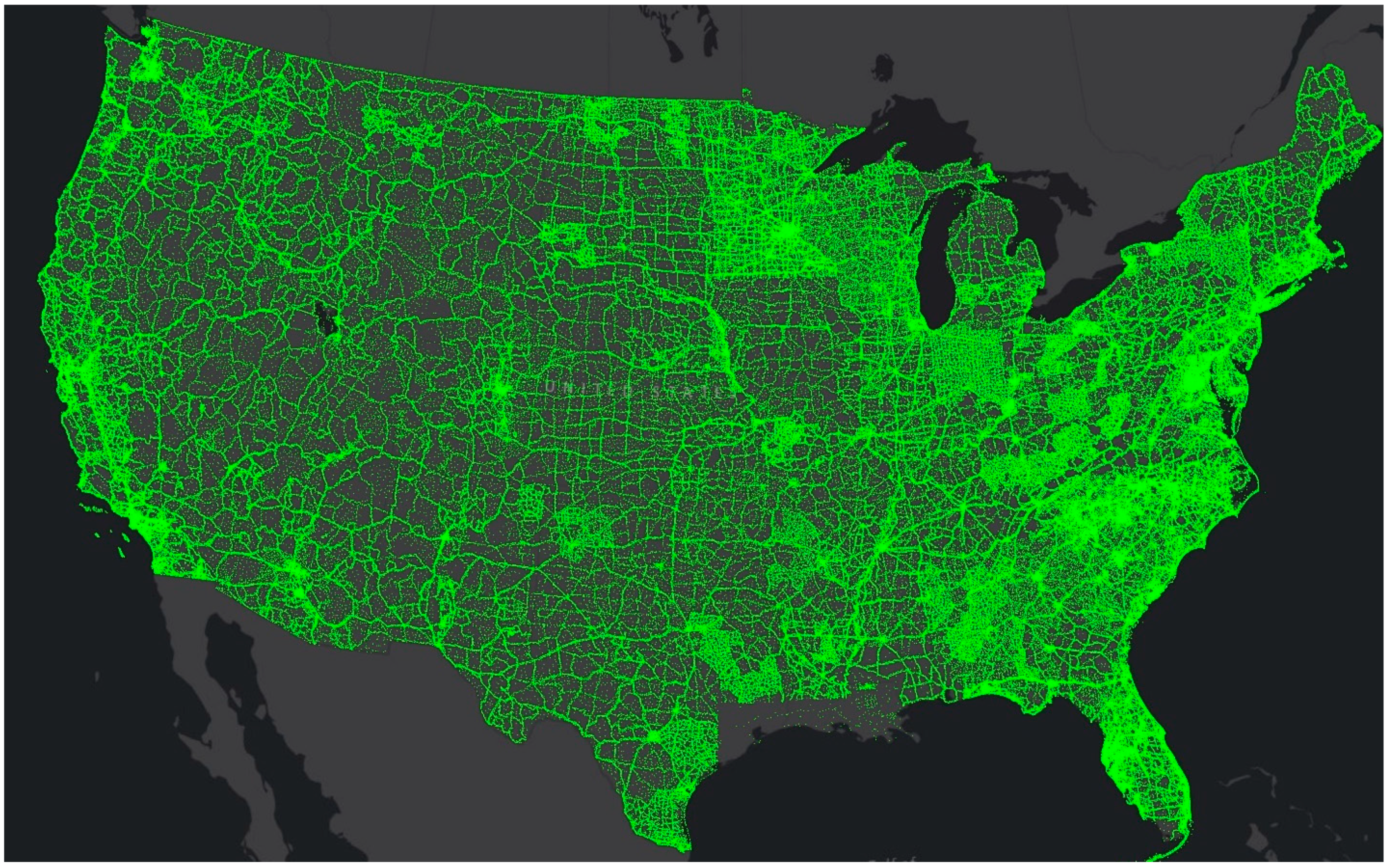
The sample design included two different approaches. First, a complete random sample (CRS) of files (
n = 4000) was selected from the master list. This number was chosen as a sample size that was feasible to analyze locally in the time allotted for this study. These LPC tiles were subsequently downloaded (
Figure 1).
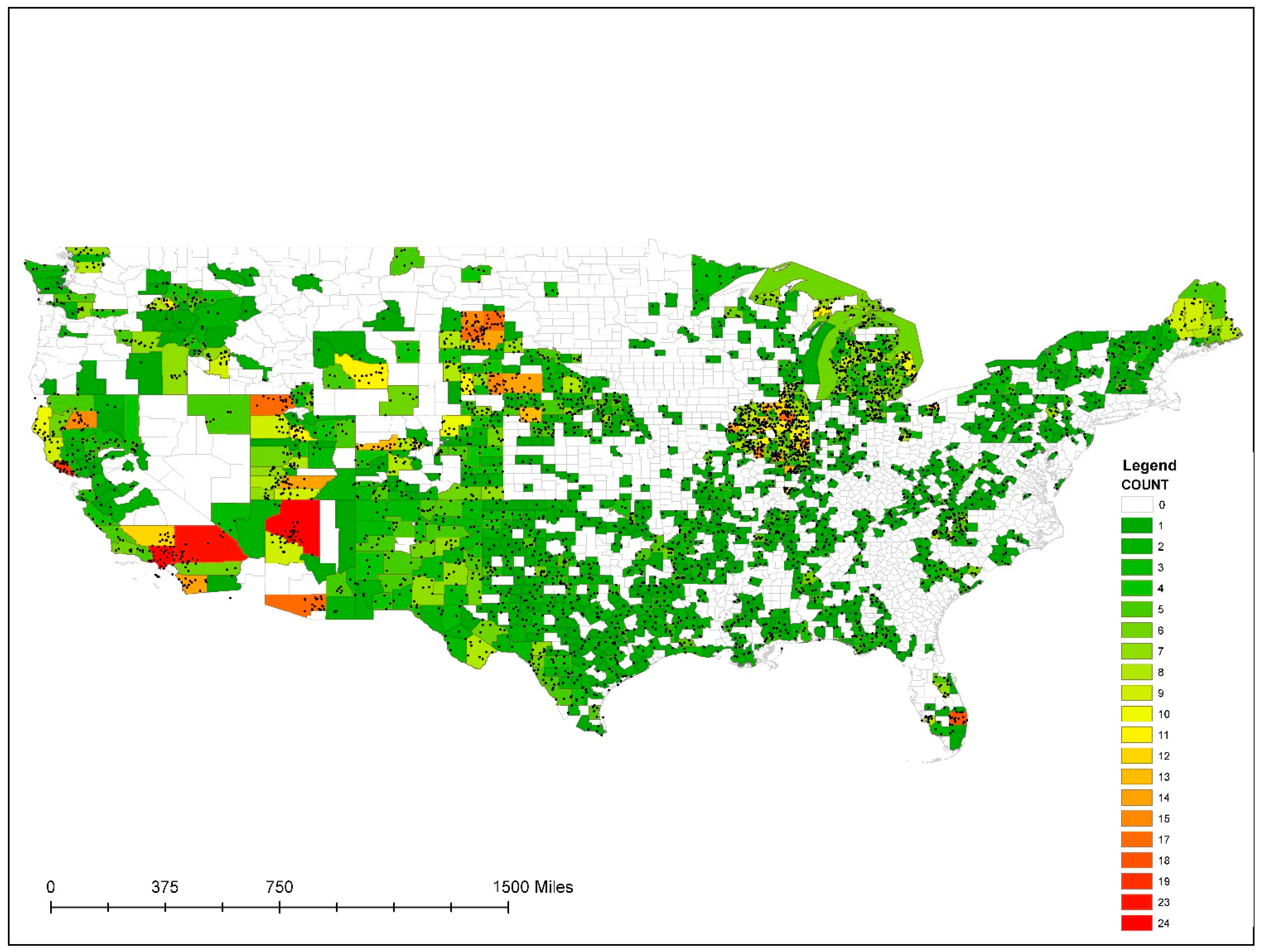
Second, a stratified random sample (SRS) was extracted from the master list, where four randomly sampled files per project (737 individual projects) were selected (
n = 2938) (
Figure 2). As project names are inherent in the file nomenclature, we were able to stratify by project by extracting the project name from the master list of files, and then randomly selecting up to four files per project. The number of files per project ranged between 1 and 84,386, with a median value of 962 files per project. Analyses were duplicated for the CRS and SRS selected files to determine if there were differences between the two sample selection methods. Only eight files were duplicates between the two sampling approaches.
The file extents differed based on the tiling scheme used for each individual project; and, therefore, sizes and extents of files, were not consistent across the entirety of the data. As a result, projects with many smaller tiles could have a larger chance of being randomly selected, giving greater influence to projects with smaller tiles. Our assumption is that the SRS method best captured the complete nature of the data in the 3DEP repository, so for the purposes of this paper some assessments were only done on the SRS files.
These files were converted to a common format and coordinate reference system. Specifically, LAZ format was converted to LAS format and projected to the CONUS Albers NAD83 (2011) [EPSG 6350] coordinate reference system. Next, all XYZ point data were integrated into a LAS dataset in Esri ArcGIS Pro (Redlands, California) for a collation of all individual file statistics.
Once all data were in Albers Equal Area, lasgrid metrics from LAStools (version 200509) were run using a 10-m cell size (a similar size to the 1/3-arc-second DEMs) to compute point densities (points per square meter; pts/m2) of points labeled as:
All points with noise removed (ignoring points classified as high and low noise);
All points excluding overlap points (points classified as overlap);
First return only;
Last return only;
Ground classified points;
Ground classified points with overlap points removed;
Z-range per cell with noise removed (a proxy for height above ground [HAG]).
Height above ground (HAG) metrics were also computed on a separate 3-m cell size using lascanopy in lasgrid using similar processes from Stoker et al. [
17]. The metrics created included (1) max HAG, (2) mean HAG, (3) STD of HAG, (4) 99th percentile height, (5) 95th percentile height, and (6) canopy cover over breast height (1.67 m), a common height threshold in forestry applications. These rasters were integrated as mosaic datasets in ArcGIS Pro*, with each point density calculation becoming its own 3DEP-wide layer.
A random sample of XY locations was created for the mosaic datasets, with a minimum distance of 10 m between sample locations to minimize double counting a single pixel. The sample points extracted the raster values from each data layer created above. The points that contained NULL values after extraction were discarded. After discarding NULL points, 854,002 sample points were available from the SRS data and 410,477 sample points were available for the CRS analysis. The difference in the number of sample points available is due to the effect of the files sizes mentioned above, where the CRS method was more likely to sample the smaller in size yet more numerous in count files. We also extracted land cover type from the National Land Cover Dataset (NLCD) to the sample points from the NLCD 2019 layer [
18].
Because files were randomly selected in both the CRS and SRS for Puerto Rico, Alaska, and CONUS, NLCD layers in Alaska (2016) and Puerto Rico (2001) were extracted, and these areas were analyzed collectively and separately, depending on the attributes selected. We looked at correlations between various attributes and derived products from the LPC data.
Lasvalidate in LAStools (version 200104)* was also run on all files to see if any large magnitude errors were in the data. Lasvalidate checked for any issues in the information provided in the header of the LAS file.
Comparisons to land cover were done in the same manner as in Stoker et al. [
17], where we used Tukey’s honestly significant difference (HSD) test to determine if the means heights by landcover classes were statistically significantly different from each other. In this case, we used the calculated Z-range values per 10-m pixel and the HAG-derived layers.
2.2. DEMs
Two versions of DEMs were evaluated—the seamless 1/3-arc-second DEM, which was downloaded and mosaicked into a single file (accessed September 2020), as well as the WCS version of the USGS dynamic elevation service (accessed April 2021). The WCS is a multi-resolution dataset, where 1-m standard DEMs (where available) are merged with 1/9-arc-second DEMs (where available) and 1/3-arc-second seamless layer into a ‘best available’ format for visualization and processing, where the highest resolution layer takes precedence. The WCS has a variable pixel resolution such that it is 1 m where there are lidar data and 10 m where there are only 1/3-arc-second data.
2.3. Survey Checkpoints
Three different survey point datasets were used for analysis. First, surveyed GNSS checkpoints provided for each individual lidar collection for 3DEP were collated into a single layer (
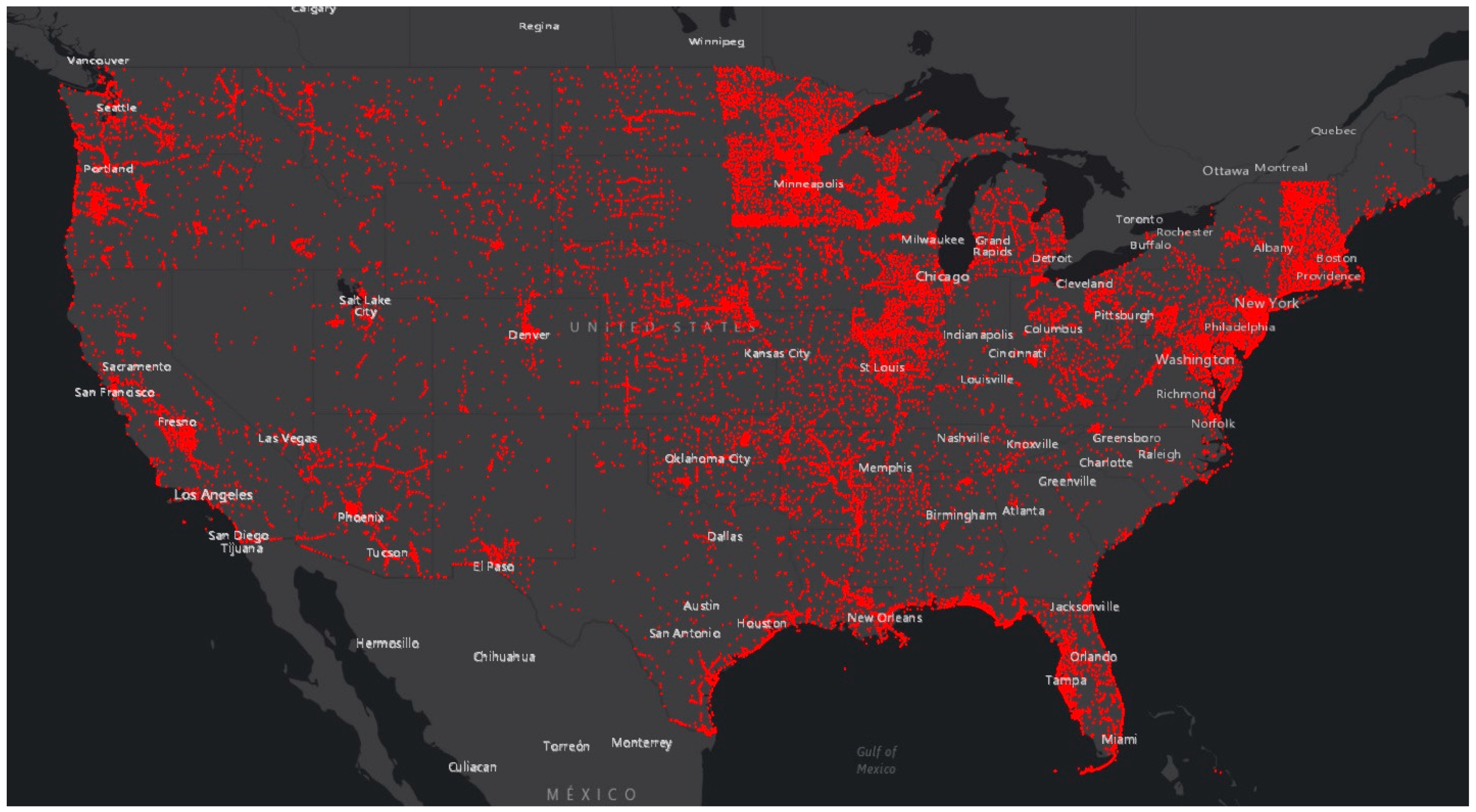
n = 53,394). These were the points used in assessing the absolute accuracy of the lidar produced for 3DEP. Second, a database of Online Positioning User Service (OPUS) points, similar to that used in Gesch et al. [
12] was created. These GPS points are survey locations loaded by surveyors into the NGS database in order to get GPS corrections (
n = 28,032)
https://geodesy.noaa.gov/opusmap/ (accessed 15 October 2021), and they would be more independent measures than the points collected directly for 3DEP. Finally, a set of survey points downloaded from
https://geodesy.noaa.gov/cgi-bin/sf_archive.prl (accessed on 15 October 2021) for all states was collated (
n = 708,833) for use. These points are the benchmarks in the NGS network. Because we were not completely sure of the quality of all these points, outliers were identified and removed using the Huber M-estimation routine in the software package JMP, using a conservative K Sigma of 6 [
19]. This resulted in a final sample size of 50,486 lidar checkpoints (
Figure 3), 24,707 OPUS points (
Figure 4), and 658,445 NGS survey points (
Figure 5). The orthometric elevation values (NAVD88) of these points were then compared to the extracted elevation values from the 1/3-arc-second seamless layer and the WCS Bare Earth DEM dynamic service. It was our hypothesis that because the WCS contained all the 1-m DEMs that have been created for 3DEP, the fit between the surveyed elevation points and the WCS would be better than the fit between the surveyed elevation points and the 1/3- arc-second DEM. Due to the geographic limitations of the 1/3-arc-second seamless DEM, our analysis on the DEMs was constrained to the CONUS.
To compare the results of the 3DEP data to other global datasets, we extracted elevation data for the OPUS point locations from the ASTER GDEM Version 3 product [
20], the NASADEM product [
15], and the SRTM Version 3.0 product [
16] available via the Application for Extracting and Exploring Analysis Ready Samples (AppEEARS)
https://lpdaacsvc.cr.usgs.gov/appeears/ (accessed on 1 October 2021). The AppEEARS application enables users to subset geospatial datasets using spatial, temporal, and band/layer parameters. Two types of sample requests are available—point samples for geographic coordinates and area samples for spatial areas via vector polygons. The sample requests submitted to AppEEARS provide users not only with data values but also associated data quality values.
To analyze the influence of lidar and resolution on the accuracy of the seamless data, we also downloaded the 1-arc-second DEM and created a 3-arc-second DEM resampled using bilinear interpolation. Next, we took the OPUS points and overlaid them with 3DEP Work Extent Spatial Metadata (WESM), which shows the extent of lidar across the United States (
https://www.usgs.gov/core-science-systems/ngp/ss/3dep-spatial-metadata [accessed on 2 February 2022]). We compared the surveyed elevation values to the various DEM cell values and then computed statistics for points that have lidar, lack lidar, and have a combined CONUS-wide computation.
4. Discussion
This study was conducted to see if limitations exist in using all the 3DEP data, both the LPCs and the derived DEMs, as a single entity. Validation testing found some issues inherent in the LPC files that were unexpected and overlooked as part of 3DEP operational data validation procedures. We found several issues that users need to be aware of when attempting to use all the lidar point cloud data together as ‘big data.’ Naming convention changes make it difficult to write scripts to process all projects. Software names were not standardized in the generating software field. This limits the ability to determine if issues were caused by specific software—one would need to prepare and simplify the data before this could be assessed. The same issue was found in the system identifier field.
The incorrect system identifier information was used in 63% of the files (n = 2529), where the software/company was listed but not the instrument. These issues make it impossible to determine if certain hardware systems were producing different data than others from the LAS files. While one could extract the hundreds of project reports to get this information, it is impossible to extract this information from the LAS file itself, which is counter to this field’s purpose.
Table 3 for the CRS and
Table 9 for the SRS both show that approximately 70% of all points were classified as either ground (~32–33%) and unclassified (~36–40%). Approximately 20% of the points had been classified as overlap. The only other class that was used substantially was high vegetation (~4%). This is because, historically, the 3DEP LPC has been the source data for bare earth DEM creation. Therefore, the focus has only been distinguishing ground versus non-ground points, water, and bridges. Value could be added to these data by classifying the unclassified points into more descriptive classifications.
Table 4 for the CRS and
Table 10 for the SRS show that most returns are first and last returns. Approximately 62% of all returns were single returns, with only 15–20% as intermediate returns and ~15% as last of many returns. A small percentage were second returns (~15%), but few returns were greater than this proportionally.
Mean point densities show that 3DEP data as a whole do meet a goal of mean ground point density of at least 2 pts/m2. To accomplish this, it appears an average of twice as many points were collected. While the 3DEP Base Specification requires at least 2 pulses per square meter (distinct from points), it appears that contractors collecting data for 3DEP have doubled the amount to ensure they meet the targets, even with overlap marked. The difference between mean and median values for both CRS and SRS samples indicates that several very high-density projects pull the mean values up, which is likely explained by the small number of QL1 projects currently in 3DEP. That being said, when looking at the 3DEP repository, quite a few sample tiles from projects (n = 50) did not meet the minimum requirement of at least 2 pts/m2. Although our sampling method was designed to provide a good representation of the overall project, these files may not be completely representative of the project as a whole, for example randomly selecting a tile that that contains mostly water.
The correlations were strong between the point density estimates and between the HAG calculations, separately. However, correlations were not significant between the point density estimates and the HAG estimates. In fact, correlation was near zero between ground point density and HAG metrics, including canopy cover. This implies that point densities, especially ground point densities, were designed and produced completely independently of the amount of vegetation in the scene. The correlation between the Z-range estimate and the HAG values was strong, especially for the maximum and 99th percentile; however, they were not a perfect match. Some of this might be explained by the difference in the cell sizes for the point density estimates (10-m) and the HAG estimates (3-m).
Breaking down point densities by land cover classes, we see that the highest point densities for non-ground points correspond with forest classes, especially evergreen forests. This make sense because a larger number of returns are needed to penetrate to the bare earth, a primary goal for 3DEP. While barren land also has a very high point density, the high standard deviations indicate that a few very high-density QL1 projects over barren lands may be skewing the mean values upward. Ground point densities appear to be fairly consistent, despite the wide range of non-ground points, implying that the vast majority of these projects were designed to achieve a certain number of bare earth points on the ground.
Comparing land cover to Z-range estimates and HAG estimates provided some insights. A general pattern was that height differences were statistically significant between most land cover classes, forested classes were the highest and cultivated crops were the lowest. This was found no matter which metric was used for comparison. However, some differences were noted when applying this approach using the 10-m Z-range estimates and the 3-m HAG estimates. The Z-range estimates show that the evergreen forest had the highest mean height (17.58 m), and it was statistically different in relation to the other forest classes; however, when comparing using the HAG layers no statistically significant differences were found between the mixed forest and the evergreen forest for maximum HAG, 99th percentile, and mean HAG. However, when using the 95th percentile HAG layer, we found significant differences between all forest classes, and the mixed forest had the highest mean height (11.22 m). These findings imply that one may get a different result based on the input height layer (which percentile) and/or what resolution the layers are, even if the land cover class is fixed at 30 m. The non-zero values found in open water in both the 10-m Z-range layer and the 3-m HAG layers, which one would assume would be zero or near zero, are understood and explained as a mixed-pixel effect in Stoker et al. [
17].
The sampling strategy also changed the result of the comparison of mean Z-range by land cover class. Using the CRS strategy, no statistical difference was found between mean Z-range of the evergreen forest (17.17 m) and the mixed forest (16.89 m); however, a significant difference was found in the SRS approach. There was little difference in mean density estimates regardless of sampling strategy. Although the SRS approach did find a wider range of issues in the individual LAS files, as it relates to computing point density there was little difference. This indicates that a completely random sample approach may not catch issues that are project-specific; however, a completely random sample approach may catch issues that are not systematic project-wide, such as differences in work units or even individual tiles.
The comparison of the surveyed points to the elevation values from the bare earth DEMs shows that the 3DEP program has continued to improve the vertical accuracy of the 1/3-arc-second seamless DEM since the last assessment by Gesch et al. [
12]. The RMSE has decreased from 1.55 m in 2013 to 0.82 m using similar OPUS points. If we look only at areas that currently have lidar data, the RMSE of 0.35 m provides a good estimate of where the final vertical accuracy value is expected to approach once the entire United States is covered by lidar data. This is an improvement for the areas that were covered in lidar in 2013, as the quality and accuracy of lidar data being ingested into 3DEP has improved over the years. Note that these points are not categorized as non-vegetated vertical accuracy (NVA) and vegetated vertical accuracy (VVA), which is why there is a difference between this result and the 10-cm RMSE value that is usually quoted for 3DEP data. A future study could categorize and re-analyze these points by presence of vegetation. The 10-cm RMSE requirement is only for NVA points on flat, open surfaces, where this estimate is much more comprehensive in nature. The 0.35-m RMSE also would include the degradation in accuracy by interpolating a 1-m (or better) DEM to a 1/3-arc-second one, which is seen in the WCS result. It is worth noting that the RMSE values of the WCS are much lower than the 1/3-arc-second seamless values (
Table 17). This is due to the nature of the service, which uses the ‘best available’ data per pixel and includes DEMs at their native resolutions, so interpolation degradation is not as pronounced. It is possible that the improvement in RMSE in the WCS versus the downloaded 1/3-arc-second is merely due to having higher resolution pixels available for elevation extraction than the interpolated seamless layer.
The residuals of the WCS versus the surveyed elevations show that many points in the OPUS and State NGS benchmarks are beyond what one would consider an understandable level of difference. Unable to completely rely on the quality of all these points, we tried to remove the most egregious outliers using statistical methods; however, many questionable points still remain. While we are unsure if these differences are a signal that warrants further checking (such as targets of subsidence or land change), we did find a project after investigating that had incorrectly been converted from feet to meters and published. Our conservative approach to retaining outliers let us find this problematic project, and 3DEP’s operations team quickly fixed the problem. We plan to continue to investigate the more divergent points to see if the error is inherent in our data or a problem with the survey.
Comparisons to other global DEM datasets such as ASTER GDEM, NASADEM, and SRTM are consistent with the findings in Gesch et al. [
12]. Independent assessments of elevation comparisons using similar but not identical OPUS points and NASA product versions gave extremely similar elevation RMSEs for the ASTER GDEM and SRTM comparisons (
Table 19). The NASADEM product was not available at the time of the Gesch et al. [
12] analysis.
5. Conclusions
This article attempts to answer questions about the consistency and ability to use all the lidar point cloud data as a single entity, and it updates the accuracy assessment of the seamless elevation models originally conducted by Gesch et al. [
12]. We found several issues that users need to be aware of when attempting to use all the lidar point cloud data together as ‘big data.’ Some notable findings were as follows:
Changes in naming conventions mid-program make it difficult to create queries based on file names alone.
The original source data had 37 different coordinate reference systems according to completely random sampling.
There were 79 different generating software packages/versions recorded according to completely random sampling.
Software names were not standardized in the generating software attribute field.
Approximately 63–68% of files had incorrect system identifier information, where the software/company was listed instead of the instrument used to collect the data.
Similar to how the software names were not standardized, the system identifiers that were populated were not consistent.
Approximately 70% of all points were classified as either ground (~32–33%) and unclassified (~36–40%), indicating a high potential for adding value by creating additional classifications.
Approximately 62% of all returns were single returns, with only 15–20% as intermediate returns and ~15% as last of many returns.
The median point densities were found to be between 3.61 and 4.20 pts/m2 for all points and between 1.87 and 2.22 pts/m2 for ground points.
Approximately 25% of projects had a sampled mean ground point density less than 2 pts/m2.
Approximately 7% of projects had a mean all point density (noise removed) less than 2 pts/m2.
While the 3DEP Base Specification requires at least 2 pulses (separate from points) per square meter, it appears that contractors collecting data for 3DEP have doubled the amount to ensure they meet the targets, even with overlap marked.
There was little difference in mean density estimates regardless of sampling strategy.
The WCS had consistently lower RMSE values than the downloaded 1/3-arc-second seamless layer, due to its use of the 1-m DEMs directly.
All point density variables contained fairly significant positive correlations, except for the Z-range variable, which only had a weak positive correlation between itself and overall point densities (noise removed and no overlap).
Height above ground assessments provide insights on the relations between height and land cover; however, further work could be done to explore the relations between sampling size and method, raster resolution, and relations with land cover.
While the stratified random sampling approach did find a wider range of issues in the individual LAS files, as it relates to computing point density there was little difference. This indicates that a completely random sample approach may not catch issues that are project-specific as it may miss a project; however, a completely random sample approach may catch issues that are not systematic project-wide.
Comparing the seamless and WCS DEMs to three different survey checkpoint datasets, we found that the 1/3-arc-second seamless layer had an RMSE between 0.35 and 1.71 m (depending on survey point dataset used); and, the WCS had an RMSE between 0.13 and 1.62 m.
Comparison to other global DEM datasets (ASTER GDEM, NASADEM and SRTM) shows that the RMSE for the 1/3-arc-second seamless (0.82 m) and WCS (0.53 m) is much better than ASTER GDEM (7.43 m), NASADEM (3.30 m), and SRTM (3.79 m), which is to be expected due to the altitudes of these systems.
The comparison of the surveyed points to the elevation values from the bare earth DEMs shows that the 3DEP program has continued to improve the vertical accuracy of the 1/3-arc-second seamless DEM since the last assessment by Gesch et al. [
12]. The RMSE has decreased from 1.55 m in 2013 to 0.82 m using similar OPUS points.
We posit that when QL2 or better lidar data are available for the entire CONUS, an overall RMSE around 0.35 m for the 1/3-arc-second seamless and around 0.13 m for a CONUS-wide 1-m dataset may be reached.
Variability by project was evident when it came to point density. Although a clear signal regarding land cover and point density was evident, the correlation between ground point density and HAG metrics, including canopy cover, was near zero. This implies that point densities, especially ground point densities, were designed and produced completely independently of the amount of vegetation in the scene. We also were able to see statistical differences between height and land cover classes; however, different calculation methods resulted in different distinctions. This could be explored further by comparing these methods to more precise height above ground measurements.
The RMSE values comparing seamless DEMs to survey control have continued to improve over time. This indicates that the lidar data being integrated into the seamless DEMs are having a verifiable improvement in accuracy. If we look only at areas that have current lidar data, the RMSE of 0.35 m provides a good estimate of where the final vertical accuracy value could approach once the entire CONUS is covered by lidar data. We posit that once lidar data are available for the entire CONUS, a nationwide RMSE of approximately this value may be reached, if not lower, as 3DEP continues to ingest higher accuracy and higher density data.
* Any use of trade, firm, or product names is for descriptive purposes only and does not imply endorsement by the U.S. Government.


