Characteristics of Marine Heatwaves in the Japan/East Sea

Abstract

Marine heatwaves (MHWs) are prolonged discrete events of anomalously warm seawater observed around the world. The occurrence of MHWs in the Japan/East Sea (JES), a middle latitude marginal sea with abundant aquatic resources, has severe impacts on marine ecosystems and human society. We used satellite remote sensing products spanning 1982–2020 to investigate the mean states and variations of JES MHWs. The results show that the JES MHWs occurred twice per year. More than 40% of the MHWs were shorter than the mean duration of 12.6 days and weaker than the mean intensity of 2.4 °C. Frequent MHWs were observed in August, while high mean intensities were observed in winter and spring in the western JES. In recent years, the area’s averaged yearly sum of MHW intensity in the JES has increased dramatically, with a positive trend of 29.62 °C days per decade—over twice the average global trend (12.37 °C days per decade), which is further confirmed by its first empirical orthogonal function mode. The strengthening trend in MHWs may be explained by oceanic dynamics rather than atmospheric forcing, and may result in increased surface latent heat flux from the ocean to the atmosphere.

1. Introduction

A marine heatwave (MHW) is defined as a prolonged anomalously warm seawater event [1]. Sea surface temperatures in the northwestern Mediterranean Sea were more than 3 °C above the long-term average temperature during the late boreal summer of 2003, which was one of the first MHWs documented in the literature [2,3,4]. MHWs can last from several days to months and cover an area thousands of kilometers wide [1,5,6]. While numerical models are sometimes used to give a future projection of MHWs, satellite observation data is most commonly used in MHW research because of its advantages of wide space, quasi-real-time and long-term results, continuity, and high temporal and spatial resolution.

In recent years, MHWs have been observed around the world from open oceans to marginal seas and coastal regions, including the Pacific Ocean [7,8], Atlantic Ocean [9,10], Indian Ocean [11,12], Mediterranean Sea [2,3,13], Bering Sea [14], China Seas [15,16,17,18], Tasman Sea [19,20,21], the west coast of the United States [22], and the southwestern Atlantic shelf [23]. These events have had severe impacts on marine ecosystems and human society, such as increasing fish mortality and bleaching coral [4,24,25,26,27]. For example, the 2011 Western Australia MHW altered the habitats of seagrasses, corals, and fish, resulting in fish deaths and the southward extension of tropical species [11,28]. The 2012 Northwest Atlantic MHW changed the distribution and population structure of longfin squid and lobster, which affected fishery resources and the economy [9,29]. The persistent 2014–2016 North Pacific MHW caused harmful algal blooms (HABs) and, via atmospheric teleconnections, affected the occurrence of extreme weather events over land, which affected human lives [7,8,22,30].

Over 90% of the excess heat generated by global warming has been absorbed by the oceans, leading to an increase in the frequency, duration, spatial extent, and intensity of MHWs [31,32]. Oliver et al. [33] found that the duration and frequency of MHWs have increased by 17% and 34%, respectively, resulting in a 54% increase in global annual MHW days from 1925 to 2016. Using satellite observations and a suite of Earth system model simulations, Frolicher et al. [6] demonstrated that MHWs in the 21st century have an average occurrence probability and spatial extent over 10 times more than they were in preindustrial times, with a significant increase in the average duration and intensity. Plecha and Soares [32] used the new Coupled Model Project Intercomparison Phase 6 (CMIP6) dataset to show a similar trend. In addition to global warming, many regional factors contribute to the growing trend of MHWs [27]. For instance, Oliver et al. [20] attributed the positive trend in MHW frequency off the coast of southeastern Tasmania to the East Australian Current, offshore anticyclonic eddies, warm air temperatures, and/or wind anomalies from northwesterly-to-easterly directions. Using numerical model results, Gao et al. [16] determined that the anomalous East Asian Summer Monsoon contributed to the increasing boreal summer MHW frequency in the East China Sea and South Yellow Sea by causing variations of shortwave radiation, ocean advection, and wind speed. Climate modes also modulate the occurrence and intensities of MHWs in some regions. For example, El Niño and La Niña events have certain promoting effects on the MHWs in China’s marginal seas and in the tropical western Pacific Ocean [18,27].

The mid-latitude regions of the Northern Hemisphere are densely populated. The impact of MHWs in these areas, especially in the mid-latitude marginal seas, is most likely to have social and economic effects. The Japan/East Sea (JES) is a semi-enclosed marginal sea located in the middle latitudes of the Northwest Pacific Ocean, bordered by South Korea to the west, Russia to the north, and Japan to the east and south (Figure 1). Significant increasing SST trends have been observed in the JES; however, the characteristics and variation of MHWs in this area are unclear. Due to the unique hydrologic properties in the JES, the MHWs in the JES have unique characteristics and distinct variation patterns. Therefore, based on a high-resolution satellite product of the daily sea surface temperature (SST), we investigated the properties, spatiotemporal distribution, long-term trends of JES MHWs, and their related causing factors.

2. Data and Methods

2.1. Data Description

Daily SST data from 1982 to 2020 at a 0.05° × 0.05° resolution were obtained from the Copernicus Marine Environmental Monitoring Service (CMEMS) (the data can be downloaded from https://resources.marine.copernicus.eu/product-detail/SST_GLO_SST_L4_REP_OBSERVATIONS_010_011, accessed on 10 January 2022). The SST data were generated from satellite data and in situ observations by the Operational Sea Surface Temperature and Sea Ice Analysis (OSTIA) [34].

The 10-m wind speed, surface net solar radiation (SSR), surface net thermal radiation (STR), surface sensible heat flux (SSHF), surface latent heat flux (SLHF), evaporation (E), total precipitation (P), significant height of wind waves (SWH), and significant height of total swell (SHTS) were investigated with respect to their contributions to the JES MHW trends. These data were provided by the European Centre for Medium-Range Weather Forecasts (ECMWF) ERA5 high-resolution reanalysis project at a horizontal resolution of 0.25° × 0.25° (the data can be downloaded from https://cds.climate.copernicus.eu/cdsapp#!/dataset/reanalysis-era5-single-levels?tab=form, accessed on 10 January 2022) [35]. The monthly Niño, Arctic Oscillation (AO), and Pacific Decadal Oscillation (PDO) index data were collected from the Koninklijk Nederlands Meteorologisch Instituut (KNMI) climate explorer at http://climexp.knmi.nl/selectindex.cgi?id=someone@somewhere, accessed on 10 January 2022 [36]. In this study, all data described above cover the period from January 1982 to December 2020.

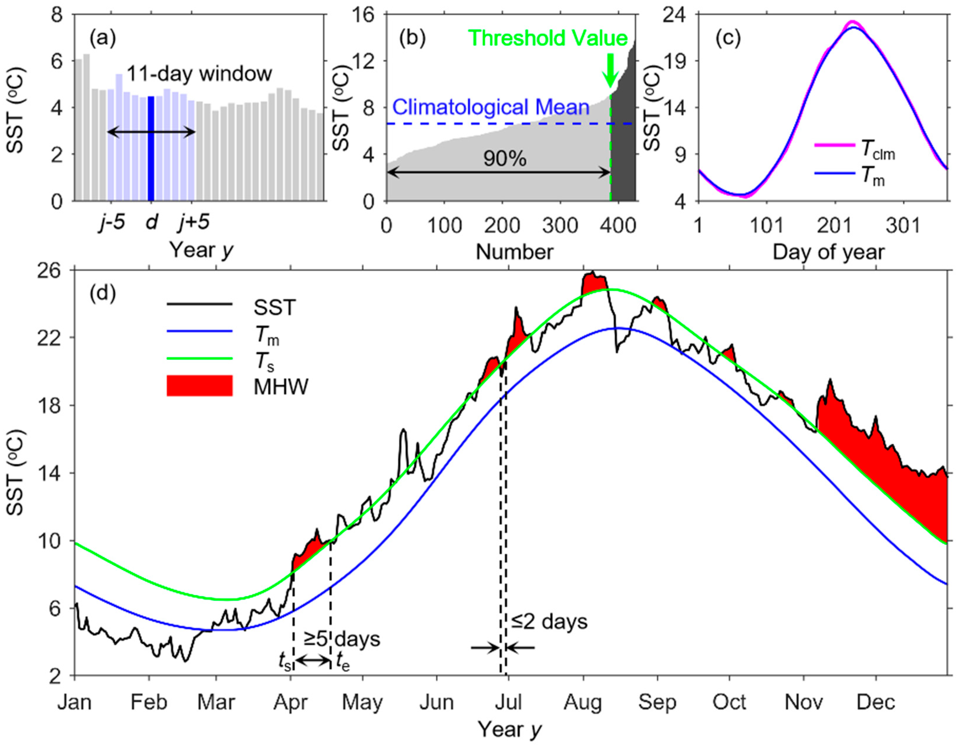
2.2. Detection of Marine Heatwaves

Hobday et al. [1] defined an MHW as a prolonged discrete anomalously warm event that lasts for at least 5 days and throughout which the SST is higher than the 90th percentile (Figure 2). For each grid point (Figure 3), the climatological mean and threshold were calculated from the daily SST data within an 11-day window centered on each calendar day (to ensure an adequate sample size) and then smoothed using a 31-day moving average [18]. Consecutive events that were less than 2 days apart were classified as the same event.

The climatological mean SST at any point grid, T_clm, is calculated as follows:

$$T_{\mathrm{clm}}\left(j\right)=\frac{1}{11\left(y_{\mathrm{e}}-y_{\mathrm{s}}+1\right)}{{\displaystyle \sum }}_{y=y_{\mathrm{s}}}^{y=y_{\mathrm{e}}}{{\displaystyle \sum }}_{d=j-5}^{d=j+5}T\left(y,d\right),$$

(1)

where T is the daily SST on day d of year y (${\mathrm{y}}_{\mathrm{s}}\ll \mathrm{y}\ll {\mathrm{y}}_{\mathrm{e}}$), j is the day of the year, y_s and y_e are the start and end dates of the climatological base period, respectively. The seasonally varying threshold SST at each grid, T₉₀, is calculated as follows:

$$T_{90}\left(j\right)=P_{90}\left(X\right),$$

(2)

where P₉₀ is the 90th percentile and $X\left(j\right)=\left\{T\left(y,d\right)\right|{ \mathrm{y}}_{\mathrm{s}}\ll \mathrm{y}\ll {\mathrm{y}}_{\mathrm{e}}, j-5\ll d\ll j+5\}$ is the SST set. The T_m and T_s are the 31-day smoothed T_clm and T₉₀, respectively. In this study, y_s and y_e are 1982 and 2020.

2.3. Marine Heatwave Indices

Once an MHW event at any grid point is detected, a set of metrics can be calculated to represent MHW characteristics, including duration and intensity. The duration of the MHW (MHWD) is the time period between the start (t_s) and end (t_e) date of the MHW. The intensity is the SST anomaly relative to the 31-day smoothed climatological mean (T_m). The I_max and I_mean are the maximum and mean, respectively, of daily intensities during the MHW [1].

An MHW event in one year can last into the following year (Figure 3d). Therefore, the number of MHWs (MHWN) in this study is the event counts from 1982 to 2020. The MHWT, MHWI, and MHWIM are the sum of MHW-day ($t_{\mathrm{MHW}}$, the day defined as an MHW), the sum of MHW-intensity ($I_{\mathrm{MHW}}, \mathrm{the} \mathrm{SST} \mathrm{anomaly} \mathrm{at} t_{\mathrm{MHW}}$), and the mean MHW-intensity from the start (D_s) to the end (D_e) date of the targeted period, respectively. In the following analysis, the MHWT, MHWI, and MHWIM over a certain month are denoted as MHWT_m, MHWI_m, and MHWIM_m. Meanwhile, the MHWT, MHWI, and MHWIM over a certain year are denoted as MHWT_y, MHWI_y, and MHWIM_y. The MHWIM reflects the mean intensity of MHWs of each day over the targeted period and actually determines the MHWI with consideration of the MHWT. All of the above MHW indices are described in detail in

Table 1. Definitions of marine heatwave (MHW) indices.

Index	Definition	Formulas	Unit
MHWD	Duration of the MHW	$\mathrm{MHWD}=$$t_{\mathrm{e}}-t_{\mathrm{s}}$ + 1	Days
Imax	Maximum intensity during the MHW	$I_{\max }=\max \left(T\left(t\right)-T_{\mathrm{m}}\left(t\right)\right)$	°C
Imean	Mean intensity during the MHW	$I_{\mathrm{mean}}=\overline{T\left(t\right)-T_{\mathrm{m}}\left(t\right)}$	°C
MHWN	Number of MHWs from ys to ye	MHWN	Occurrences
MHWT	Sum of MHW-day from Ds to De	$\mathrm{MHWT}={\displaystyle {\displaystyle \sum }_{D_{\mathrm{s}}}^{D_{\mathrm{e}}}}{t}_{\mathrm{MHW}}$	Days
MHWI	Sum of MHW-intensity from Ds to De	$\mathrm{MHWI}={{\displaystyle \int }}_{D_{\mathrm{s}}}^{D_{\mathrm{e}}}{I}_{\mathrm{MHW}}d{t}_{\mathrm{MHW}}$	°C Days
MHWIM	Mean MHW-intensity from Ds to De	$\mathrm{MHWIM}=\mathrm{MHWI}/\mathrm{MHWT}$	°C

.

2.4. Ekman Pumping

The Ekman pumping vertical velocity is calculated as follows:

$$w_{\mathrm{E}}=-\nabla \times \left(\frac{\tau }{{\rho }_{0}f}\right),$$

(3)

where τ is the wind stress calculated from the 10-m wind data of ECMWF ERA5, ${\rho }_0$ is the mean sea water density, which was taken to be 1.025 × 10³ kg/m³, and f is the Coriolis parameter.

2.5. Net Surface Heat and Freshwater Flux

The net surface heat flux (SHF) is an important variable for understanding air–sea interactions. It is expressed as the following equation:

$$\mathrm{SHF}=\mathrm{SSR}+\mathrm{STR}+\mathrm{SSHF}+\mathrm{SLHF}.$$

(4)

The freshwater flux (SWF), which is the difference between the E and P, is computed as follows:

$$\mathrm{SWF}=\mathrm{E}+\mathrm{P}.$$

(5)

The SSR, STR, SSHF, SLHF, E, and P data were all obtained from the ECMWF ERA5, with the downward direction set to be positive. That is, a positive (negative) SHF represents ocean gain (loss) of heat, and a positive (negative) SWF represents precipitation (evaporation).

2.6. Empirical Orthogonal Function Analysis

The Empirical Orthogonal Function (EOF) analysis is commonly used for time series analysis to reveal possible spatial patterns of climate variability and how they change with time, and was conducted using the Climate Data Toolbox for MATLAB developed by Greene et al. [37]. The EOF method was used to reveal the spatiotemporal variability in the JES MHWs and explain the MHW variability in the South China Sea [18] and off of eastern Tasmania [20]. In this study, MATLAB software was used for calculation and analysis.

3. Results

3.1. Statistical Characteristics

On average, there were about two MHWs in the JES during the period from 1982 to 2020. A high MHWN occurred in the southwestern JES and a low MHWN occurred in the Japan Basin (Figure 4a). The average MHWT_y peaked at more than 26 days in the western JES at approximately 40° N (Figure 4b). Except for the Tsushima Strait, the mean MHWD was more than 10 days over the entire JES and was more than 15 days in the central JES and along the North Korea coast (Figure 4c). The longest MHW event occurred off the east coast of North Korea, lasting more than 200 days from August 2019 to the spring of 2020. The spatial patterns of the mean I_max and I_mean are similar to that of the average MHWT (Figure 4d,e), with high values (over 4 °C and 3 °C, respectively) in the western JES.

Lifetime and intensity are important parameters for describing the characteristics of MHWs. The mean MHWD and mean I_mean of all MHWs in the JES were 12.6 days and 2.4 °C, respectively, which are represented by the dot–dash line and the dashed line, respectively, in Figure 5. The probability density function (PDF) distribution is divided into four regions by these two lines. Beginning at the top right quadrant and moving counterclockwise, the values account for cumulative PDFs of 17.8%, 12.9%, 41.8%, and 27.5%. These statistical results show that MHWs of short duration and weak intensity prevail in this region, where the most frequently occurring MHWs have a duration of 5 days and a mean intensity of 2.1 °C.

3.2. Seasonal Variability

The average JES MHWT_m varied from 0 to more than 6 days, showing strong seasonal variability (Figure 6). MHW events occurred in all seasons in the JES, with a high MHWT_m in summer (from June to August), and a low MHWT_m in spring (from February to May). In January and February, the spatial distribution of the MHWT_m was similar, with low values in the Tartar Strait and the southeastern coastal region (Figure 6a,b). In April, the MHWT_m in the Japan Basin decreased significantly (Figure 6d). The MHWT_m was at a low level from April to May, with high values (more than 2 days) in the North Korea coastal area (Figure 6d,e). Spatially, the MHWT_m in June showed a meridional distribution pattern of being high in the south and low in the north (Figure 6f). The MHWT_m increased in July, except in the southeastern JES (Figure 6g). The frequency and spatial extent of MHWs both reached their annual maximums in August (Figure 6h). The MHWT_m in June showed a zonal spatial distribution pattern of being high in the east and low in the west (Figure 6i). From October to December, the level and spatial distribution of the MHWT_m were roughly similar to those from January to March (Figure 6j–l).

In contrast to the MHWT_m and MHWI_m, the seasonal variability of the average MHWIM_m was reflected mainly in its spatial distribution (Figure 7). In winter and spring, the MHWIM_m was spatially distributed more inhomogeneously than in summer and autumn. The MHWIM_m varied from 0.01 °C to more than 5 °C in winter, with high values in the western JES and low values in the Tartar Strait and southeastern JES. In spring, the inhomogeneity of the spatial distribution decreased, the maximum MHWIM_m decreased to 4 °C, and the minimum MHWIM_m increased to 1.7 °C. The variation range and regional differences of the MHWIM_m were the smallest in summer. The inhomogeneity increased in September, with a high-value area in the eastern JES. In October and November, the distribution of a high MHWIM_m was scattered. A low MHWIM was observed mainly in the southeastern JES.

Figure 8 shows that the average MHWI_m was high in summer and low in spring, which is consistent with the seasonal variation of MHWT_m. By comparing the seasonal variation of the spatial distribution of MHWI_m and MHWT_m, it can be found that the distribution characteristics of the two are relatively similar between June and October. This pattern means that the MHWI_m was mainly affected by the MHWT_m in this period. In the other months, a high MHWI_m (more than 5 °C days) was observed in the subpolar front area around 40° N, especially in the coastal regions near North Korea.

Although the spatial distributions of the average MHWT_m, MHWI_m, and MHWIM_m are different, they have similar seasonal variations in temporal distribution, with the maximums appearing in summer (Figure 9). Due to the high frequency of MHWs in August, the MHWT_m reached a maximum of 4.6 days. Because of the wide spatial extent of MHWs in August, the MHWI_m reached a maximum of 12.6 °C days. This explains why many studies focus only on the summer MHWs [18]. However, the seasonal variation in the MHWIM_m is weak, with the maximum of 2.8 °C occurring in July and the minimum of 2.0 °C occurring in February.

3.3. Interannual Variability and Long-Term Trends

In addition to seasonal variations, the JES MHWs also showed interannual variabilities during the 1982–2020 period (Figure 10). The frequency of MHWs in the JES was relatively high, with MHWs occurring in all months except for June 1983, October 1984, June 1986, and May 1987. Moreover, the MHW frequency increased significantly in the most recent years, which is clearly reflected in the temporal distribution of the high MHWT_m and MHWI_m. With the exception of 2019 and 2020, the JES MHWs tended to occur in summer. Compared to the interannual variation of the MHWT_m and MHWI_m, the interannual variation of the MHWIM_m is weak.

Significant positive trends in the MHWT_y occurred almost throughout the JES region (Figure 11a). A rapidly increasing trend of over 15 days/decade was found in the area south of 45° N in the JES. The annual regionally averaged MHWT_y time series shows a rapidly increasing trend at 12.01 ± 3.48 days/decade, passing over a significance level of p < 0.01 (Figure 11b). Positive trends in the MHWI_y were also found almost across the entire area of the JES, with high trends of more than 90 °C days/decade appearing in the western corner of the JES (Figure 11c). Additionally, the annual area-averaged MHWI_y time series shows a rapid growth trend of 29.62 ± 9.00 °C days/decade (p < 0.01), which is consistent with the annual area-averaged MHWT_y (Figure 11d). Although the trends of the MHWIM_y are basically positive in the whole JES, the linear trend in the regional averaged time series is only 0.07 ± 0.07 °C/decade, with a relatively weak significance level of p < 0.05 (Figure 11e,f).

The MHWI_y, including the properties of frequency, duration, and mean intensities of the MHWs, is a comprehensive index for measuring MHWs [18]. Therefore, EOF analysis was conducted on the MHWI_y to reveal the spatiotemporal patterns of JES MHWs. The first three leading modes respectively account for 44.89%, 15.49%, and 6.23% of the total variance. The first EOF mode (EOF1) essentially represents basin-scale trends in the JES MHWI_y (Figure 12). The EOF1 pattern is reminiscent of the spatial distribution of trends in the MHWI_y, showing positive values throughout the JES, with high values in the western corner and center of the JES (Figure 11c and Figure 12a). The corresponding time coefficients of EOF1 (PC1) show an increasing trend above the 99% significance level (p < 0.01), with a turning point in approximately 2004.

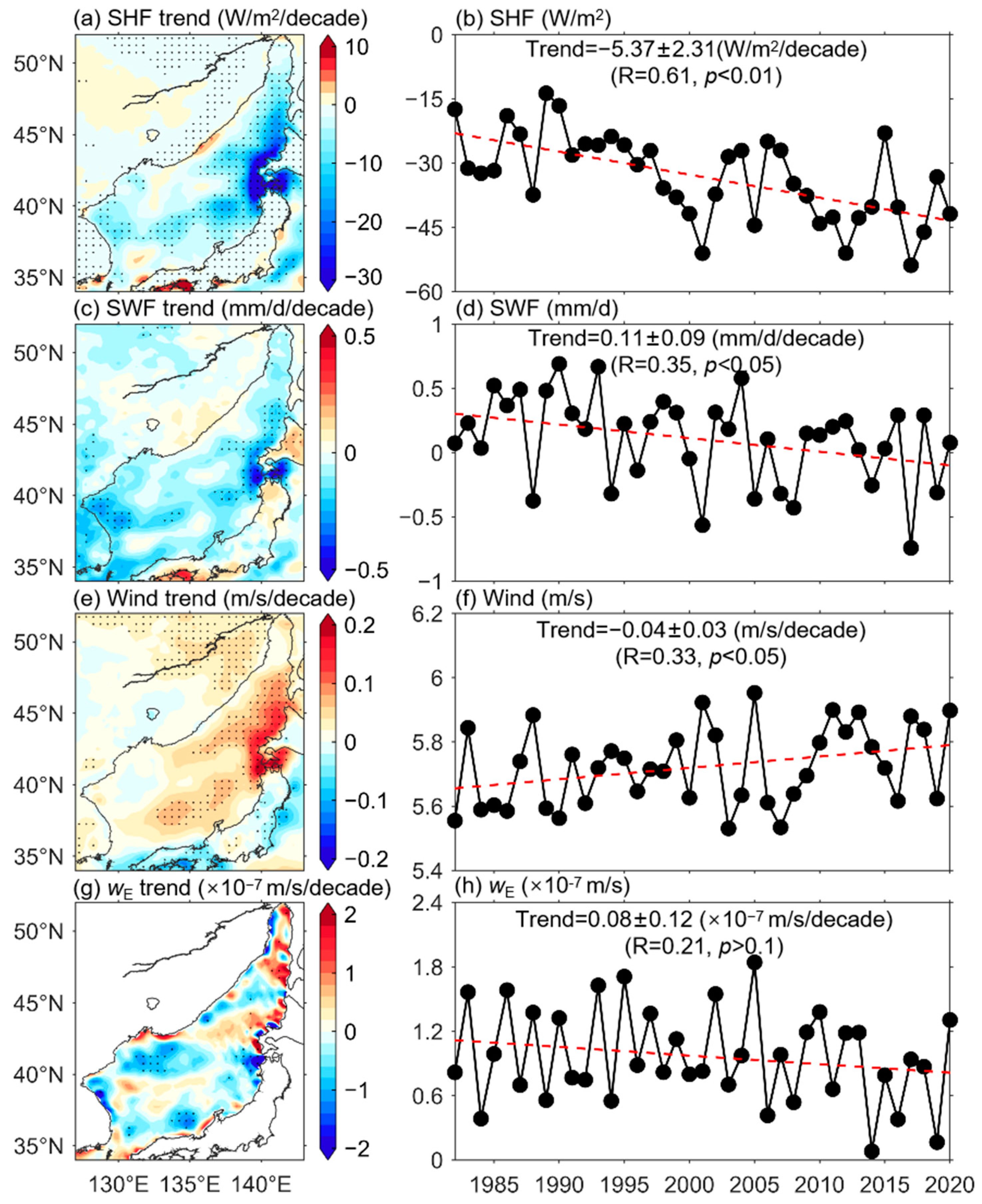
3.4. Factors Associated with Long-Term Trends in Marine Heatwaves

Previous investigations have qualitatively discussed the potential variables associated with the occurrence of MHWs, including climate modes, air–sea heat fluxes, mixing processes, and Ekman pumping [5,33,38,39,40,41]. The correlations between the PC1 and the PDO index, the AO index, and the Niño index are −0.29, 0.13, and −0.01, showing that the PDO, AO, and El Niño–Southern Oscillation (ENSO) had no significant correlation with the JES MHWs. However, the average MHWT_y values of the PDO positive phase years were relatively lower than those of the PDO negative phase years. Furthermore, the spatial distribution of the average MHWT_y values between positive and negative AO phase years is different. Figure 13c shows a dipole-like pattern, with high values identified in the northwestern JES and low values identified in the southern and southeastern JES; the pattern is shifted in Figure 13f. Compared to the PDO and AO, the ENSO had a relatively weak effect on the JES MHWs (Figure 13d,g).

We explored variations in the SHF, SWF, wind speed, and $w_{\mathrm{E}}$, as shown in Figure 14. The SHF of almost the entire JES region shows significant negative trends, indicating that the ocean was sending heat to the atmosphere, especially in the area of the Tsugaru Strait (−30 W/m²/decade) (Figure 14a). The annual regionally averaged SHF time series in the JES shows a decreasing trend of −5.37 ± 2.31 W/m²/decade at a significance level of p < 0.01 (Figure 14b). Meanwhile, the SWF and 10-m wind speed have negative and positive trends in the area of the Tsugaru Strait, with area-averaged trends of 0.11 ± 0.09 mm/d/decade and −0.04 ± 0.03 m/s/decade, respectively. Due to the inhomogeneous spatial distribution of the trends in ${\mathit{w}}_{\mathrm{E}}$, the corresponding area-averaged trend is relatively weak, below the 90% significant level. Since a significant increasing trend of the annual area-averaged time series of the SHF was observed, we studied the variations of each component of the SHF further.

The weak increasing trends of the SSR were observed in most of the JES except for the area of Tsugaru Strait, with a regionally averaged linear trend of 0.70 ± 0.72 W/m²/decade (Figure 15a,b). The STR shows significant decreasing trends in the northeastern JES region, indicating that the surface net upward longwave flux had an increasing trend (Figure 15c). The annual regionally averaged STR time series in the JES shows a decreasing trend of −0.76 ± 0.42 W/m²/decade at a significance level of p < 0.01 (Figure 15d). Meanwhile, the decreasing trends of the SSHF also hold in the eastern JES, with area-averaged trend of −1.27 ± 1.10 W/m²/decade above a 95% significant level (Figure 15e,f). Decreasing trends in the SLHF were found across almost the entire area of the JES, indicating that the surface upward latent heat flux of the JES had positive trends from 1982 to 2020 (Figure 15g). A relatively faster trend of −4.05 ± 1.17 W/m²/decade was observed in the area-averaged SLHF above a 99% significant level (Figure 15h).

In addition, we explored the correlations between the PC1 and the variables and processes associated with air–sea interaction (Figure 16). As shown in Figure 16a, the SHF in most areas of the JES was negatively correlated with PC1, with a high correlation coefficient of −0.7 (p < 0.01) in the west of the Tsugaru and Soya Straits, indicating that the ocean had a forcing effect on the atmosphere. Compared to the SSR, STR, and SSHF, the SLHF had a relatively stronger correlation with the PC1, showing that the ocean affected the atmosphere mainly by releasing surface latent heat flux upward. Meanwhile, the weak negative correlation between the SWF and the PC1 was mainly due to the increase in E, which is consistent with the variation of the SLHF. However, the mixing processes had no significant impact on the positive trend of the JES MHWI_y (Figure 16i–l).

4. Discussion and Conclusions

The MHWs in the JES are samples of enhancing MHWs over the world. As shown in Figure 17a, compared to the rest of the world, the MHW frequency in the JES is at a moderate level, with an area-average MHWN of 1.97 occurrences, which is slightly higher than the global averaged level of 1.82 occurrences (

Table 2. Mean states and trends of area-averaged marine heatwave (MHW) indices from 1982 to 2020.

Area (Longitude and Latitude Range)	Average MHWN (Occurrences)	Average MHWTy (Days)	MHWIy (°C Days)	MHWTy Trend (Days/Decade)	MHWIy Trend (°C Days/Decade)
Global (0°–360° E, 90° S–90° N)	1.82	63.12	32.69	8.54	12.37
Japan/East Sea (127°–145° E, 32° N–52° N)	1.97 (10) *	24.86 (11)	59.65 (3)	12.01 (9)	29.62 (3)
Equatorial Pacific cold tongue (180°–280° E, 5° S–5° N)	1.17	30.77	67.13	−3.36	−11.95
East China Seas (100°–127° E, 25° N–40° N)	2.12	23.92	45.65	11.88	23.44
South China Sea (100°–121° E, 0° N–13° N)	2.33	26.18	32.19	12.05	14.41
Bay of Bengal (80°–90° E, 5° N–22° N)	2.27	23.94	25.14	10.08	10.21
Arabian Sea (45°–79° E, 0° N–28° N)	2.06	24.83	31.64	13.88	18.21
Gulf Stream (280°–320° E, 32° N–50° N)	2.12	26.04	58.05	13.54	27.95
South coast of Africa (0°–80° E, 45° S–32° S)	2.11	25.98	49.39	4.82	11.15
East coast of South America (310°–335° E, 50° S–35° S)	2.13	26.13	47.78	8.81	16.74
Mediterranean Sea (0°–30° E, 30° N–45° N)	1.92	24.86	45.32	16.31	29.90
Gulf of Mexico and Caribbean (260°–290° E, 10° N–30° N)	2.05	24.69	31.00	14.71	17.74
East coast of Australia (140°–170° E, 45° S–30° S)	1.94	26.70	42.30	12.41	21.96
Indonesian sea (105–135° E, 10° S–0° S)	2.27	27.97	31.65	13.36	14.68
Western North Pacific Ocean (135°–225° E, 30° N–45° N)	1.82	28.05	59.92	14.30	30.99
Sea of Okhotsk (135°–165° E, 42° N–64° N)	1.83	26.68	45.94	11.16	20.84

* The numbers in brackets indicate the rank of the Japan/East Sea (JES) averaged marine heatwave (MHW) index among the area-averaged MHW index for all regions in Table 2.

). Globally, except among the Arctic and Antarctic regions, the average MHWT_y ranges around 23.92–30.77 days, similar to the JES. The increasing trend of the area-averaged MHWT_y in the JES is about 12.01 days/decade, exceeding that of the global averaged MHWT of 8.54 days/decade. Although the spatial distributions of increasing trends in the MHWT_y and the MHWI_y are similar in the JES (Figure 17c,d), the increasing trend in the MHWI_y is relatively strong, reaching 29.62 °C days/decade, which is slightly slower than that in the Mediterranean Sea and in the western North Pacific Ocean. Taking into consideration the rather high baseline of the MHWI_y, which already reached an area-averaged value of 59.65 °C days, this significant increasing trend of the MHWI_y highlights the importance of MHWs in the JES and suggests the need for further studies.

Many studies have revealed increasing trends in the frequency, duration, and intensity of MHWs due to global warming [31,32]. Indeed, as the definition of MHWIy index goes, the PC1 of the MHWI_y coincided with the area-averaged yearly SST anomalies, with a significant correlation coefficient of 0.77 (p < 0.01). Compared to the global averaged SST trend (0.12 °C/decade at a significance level of p < 0.01), the SST trend in the JES is much stronger, especially in the central JES (Figure 1). Furthermore, even if the global averaged SST trend is removed from the daily SST for each grid point, the increasing trends in the MHWT_y and MHWI_y also hold throughout the JES after rerunning the MHW analysis following the same procedures as we did for the original SST data, with area-averaged increasing trends of 6.07 days/decade and 16.69 °C days/decade, respectively.

MHWs show that various scale changing patterns and climate modes are promising candidates to explain the causes of variation in MHWs. Indeed, the results show that the PDO, AO, and the El Niño–Southern Oscillation (ENSO) have no significant correlation with the significant increasing trend in the MHWI_y [14]. However, the average MHWT_y values in the positive PDO phase years were higher than those in the negative PDO phase years. During the positive phases of the PDO, the JES was generally in a cooler state in the upper layer, thereby suppressing the occurrence of MHWs [42,43,44]. A positive AO phase generally led to a weaker East Asia winter monsoon and a warmer winter over the JES [45,46,47]; as a result, the MHWs in the northern JES were slightly more active than in the southern JES because of the weakened wind speeds and decreased sea ice induced by the positive AO phase.

Besides climate modes, some of the most likely causes of marine heatwaves are ocean currents. Along the Tsushima Strait, there is a perennial circulation from the southwest toward the northeast, referred to as the Tsushima Warm Current (TSWC), which is the only inflow for the JES, a semi-enclosed marginal sea. Additionally, the majority of the TSWC flows out through the Tsugaru Strait into the Pacific Ocean, and through the Soya Strait into the Okhotsk Sea, known as the Tsugaru Warm Current and the Soya Warm Current, respectively [48,49]. Therefore, the water temperature anomalies are closely related to the variations in the TSWC of both the volume transport and the pathways. Under positive PDO conditions, the water transport of the TSWC was decreased, leading to a reduction in the heat supply to the JES, and thereby resulting in relatively fewer MHWs than under the negative phase of the PDO [42,43]. Besides variation and along with climate modes, an increasing trend of 0.1 Sv per decade was observed not only in the ADCP measurements but also in the sea-level differences across the Tsushima Strait [50]. However, due to the scarcity of in situ observations, it is too soon to jump to the conclusion of the relationship between the ocean currents and MHWs, which may need to be further evaluated by high-resolution coupled models.

The strengthening trends of MHWs may have vital importance for human activities. The long-term trend in JES MHWs reflects that the ocean has a forcing effect on the atmosphere, which causes increases in the surface temperatures in the surrounding lands, increasing the occurrence of land heatwaves [51]. Moreover, the high amplitude area in the EOF1 of the MHWI_y is located in the western JES around 40° N, where fishing resources are rich due to the interaction of warm and cold currents. The warmer environment could alter the habitats of fishes, and the likely induced HABs could result in fish deaths. Due to a sudden increase in the water temperature in the upper layer (50–100 m) in 1987–1989, a shift of fish assemblage structure occurred in 1998–1989, such that the common squid became the dominant species of commercial fish catches (over 60%) instead of filefish, anchovy, and sardine in the Tsushima Basin after 1993 [52]. The MHWs’ environmental and economic significance may be also subjected to MHWs’ influential depth, besidesds their duration and intensity. In addition, strong subsurface MHWs have been observed in the tropical western Pacific Ocean based on buoy data [27]. However, due to the lack of temperature profile data, the depth of the impact of the MHWs is unclear so far and requires further comprehensive field observation.

5. Summary

In this study, we used newly released high-resolution satellite daily SST data from 1982 to 2020 to investigate the characteristics of JES MHWs, including the mean states, seasonal and interannual viabilities, and the long-term trends. Our results are summarized as follows:

(1)

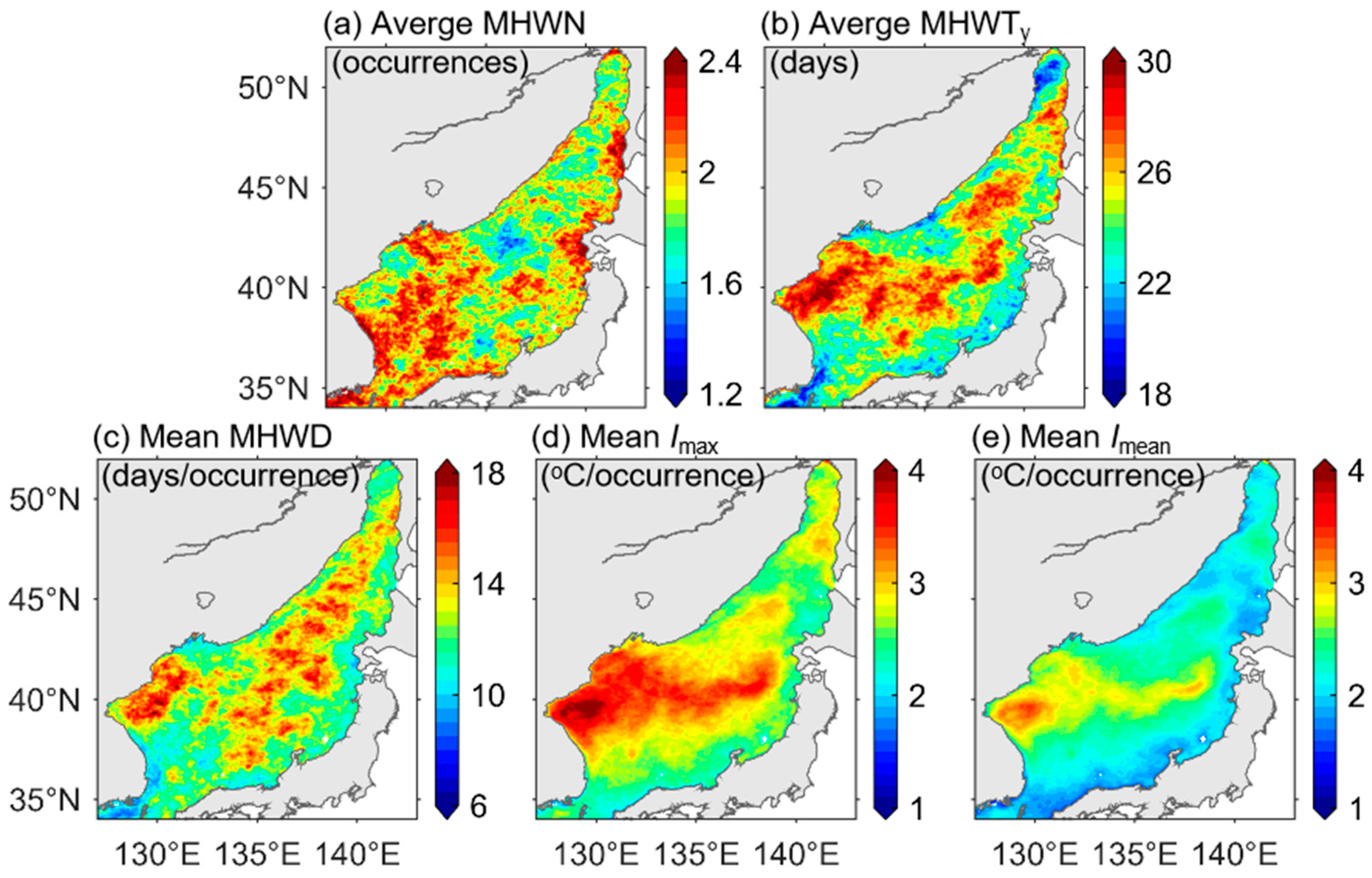
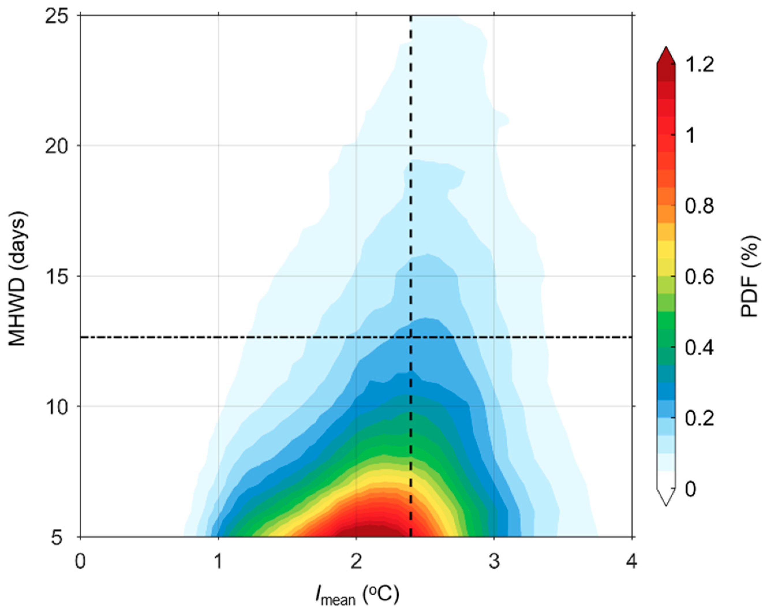
JES MHWs occurred about twice per year, with a mean MHWD and a mean I_mean of 12.6 days and 2.4 °C, respectively. MHWs with a short duration and weak intensity dominated in this region. A duration of 5 days and a mean intensity of 2.1 °C were particularly common. High MHWT_y and high SST anomalies were both observed in the western JES at approximately 40° N.

(2)

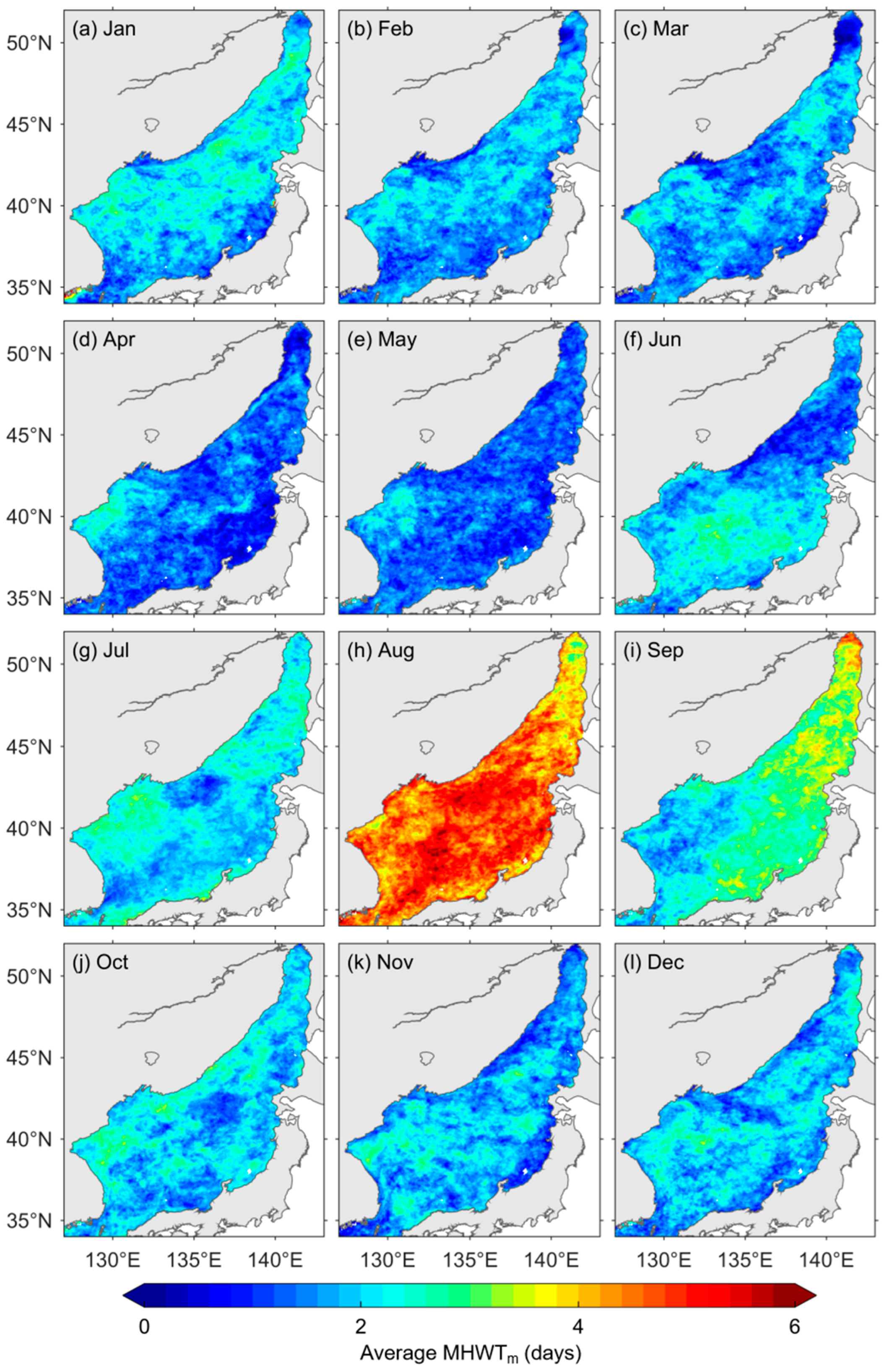
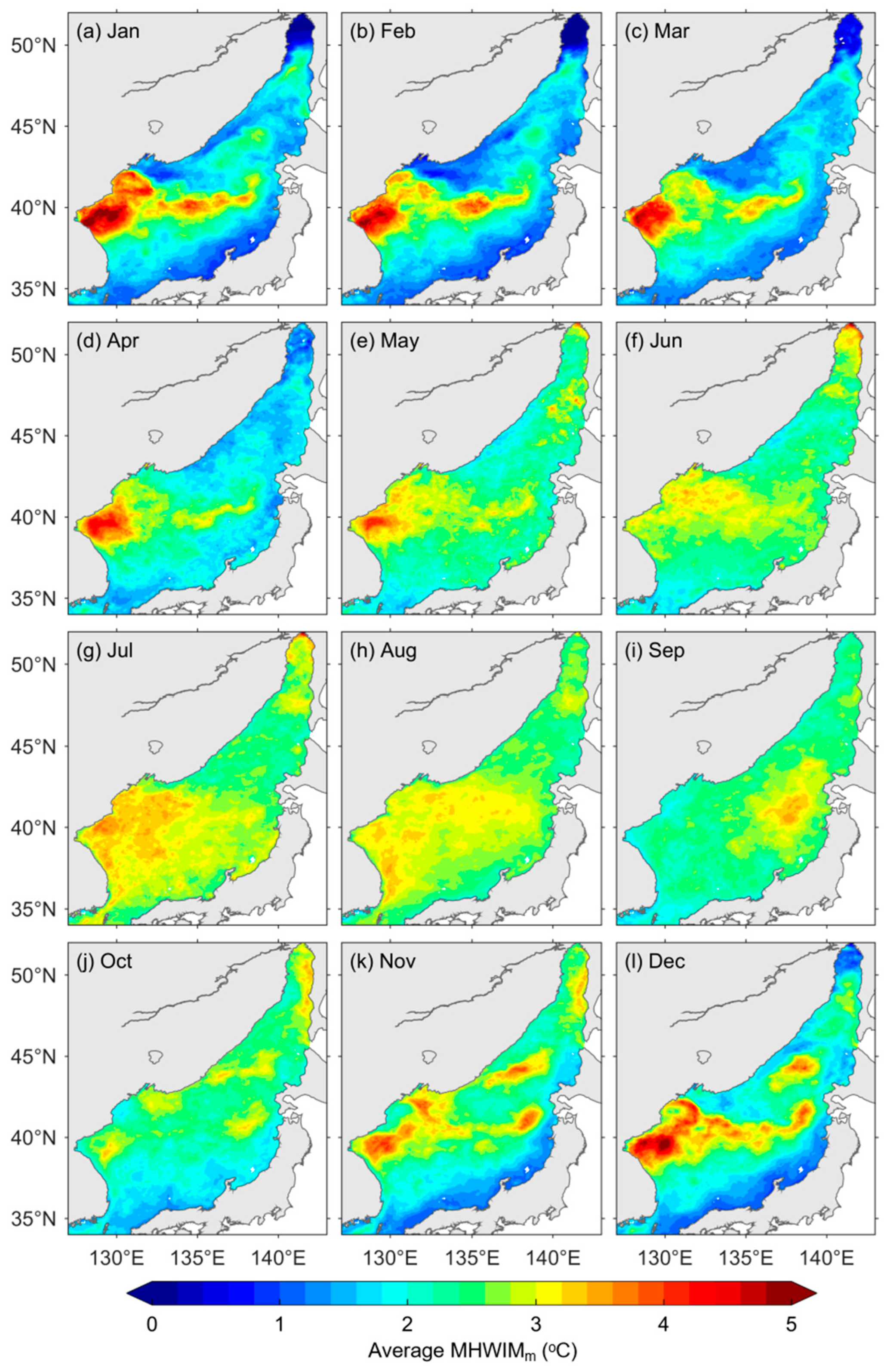
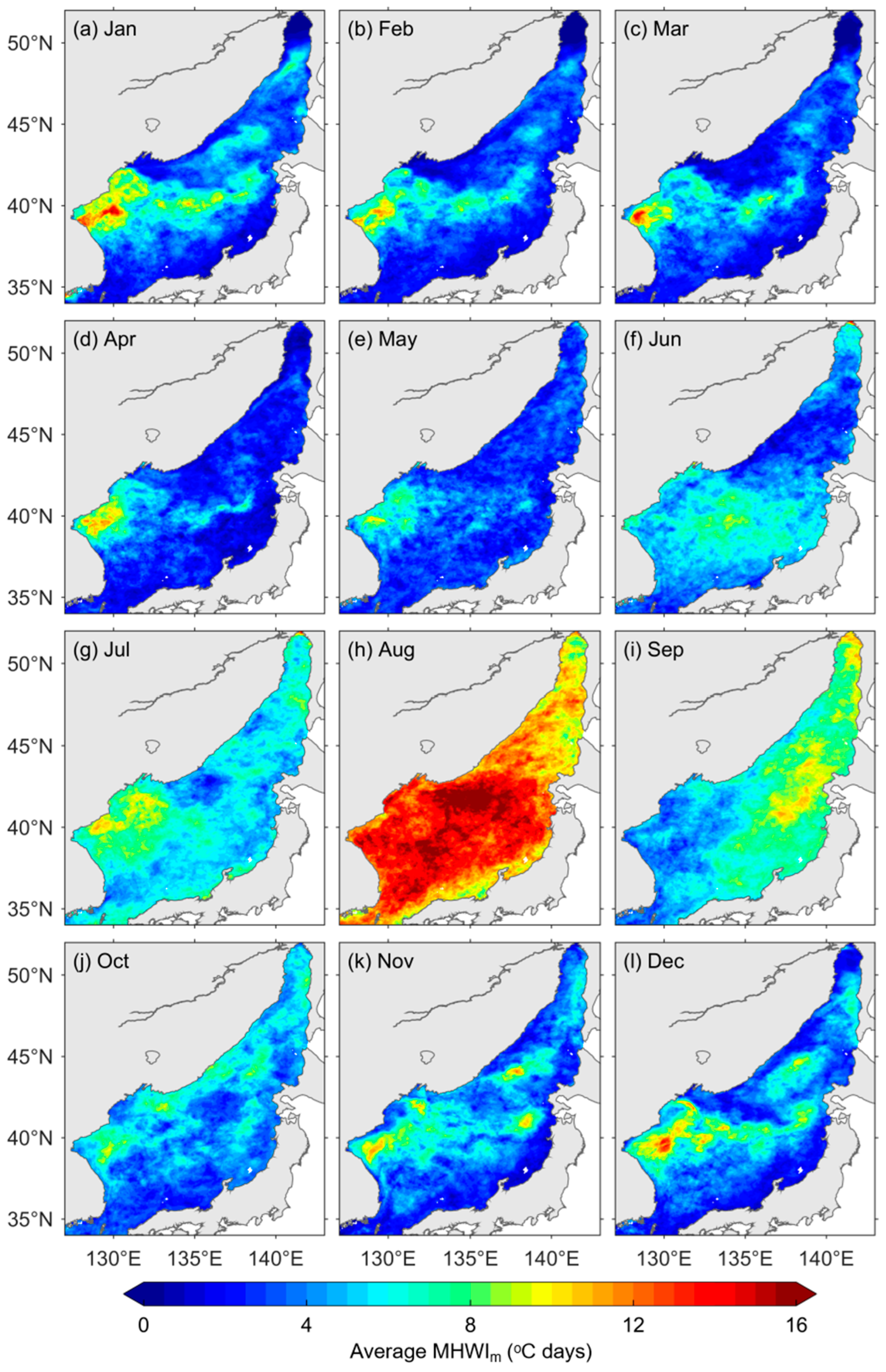
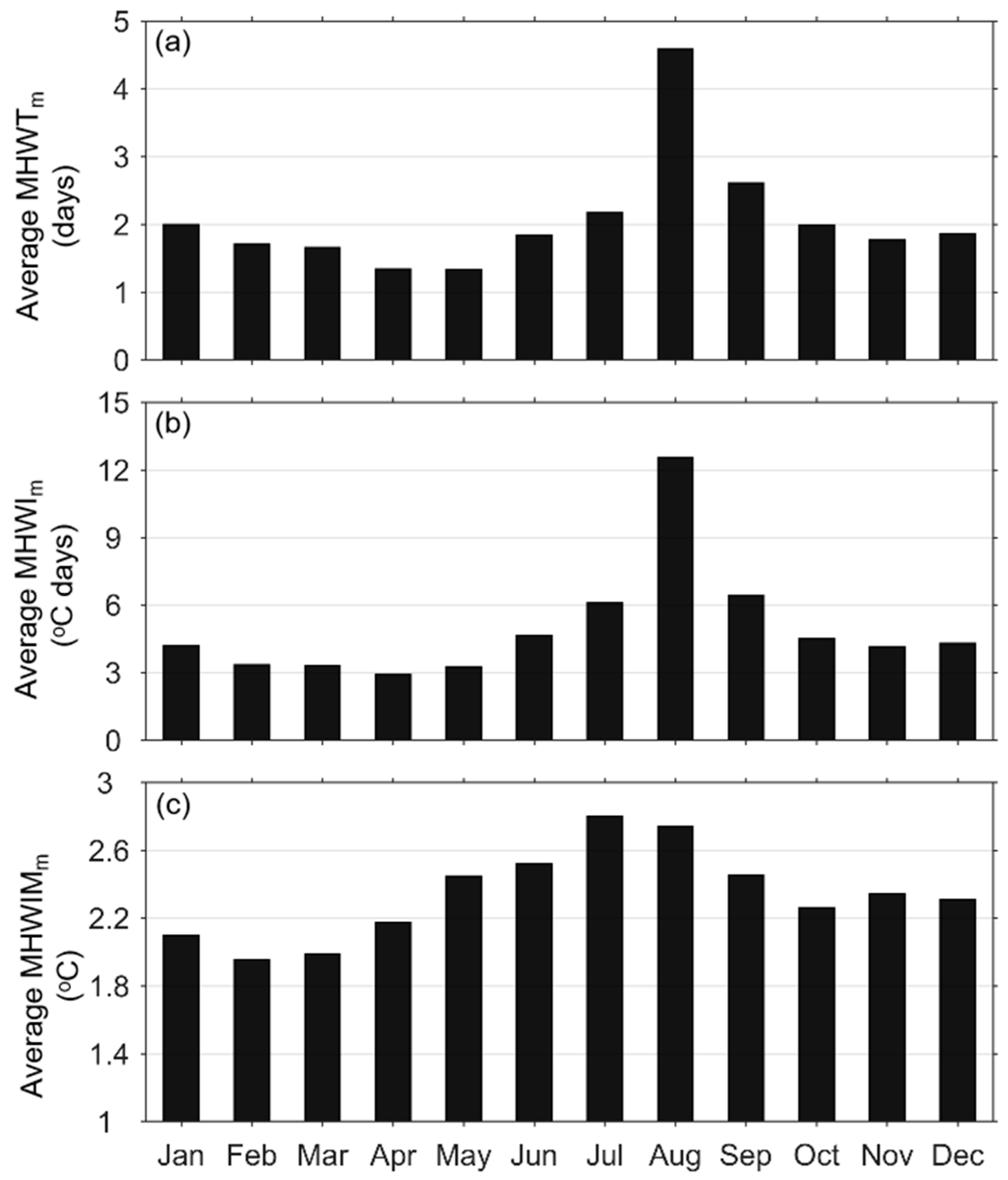
Both the spatial and temporal distributions of MHW indices were subject to strong seasonal variability. The maximum values of the regional averaged MHWT_m, MHWI_m, and MHWIM_m (4.6 days, 12.6 °C days, and 2.8 °C, respectively) all occurred in August. However, a high MHWI_m and MHWIM_m in the western corner of the JES also appeared in winter (from December to February) and spring (from May to March). The MHWs in the eastern JES were also active in September.

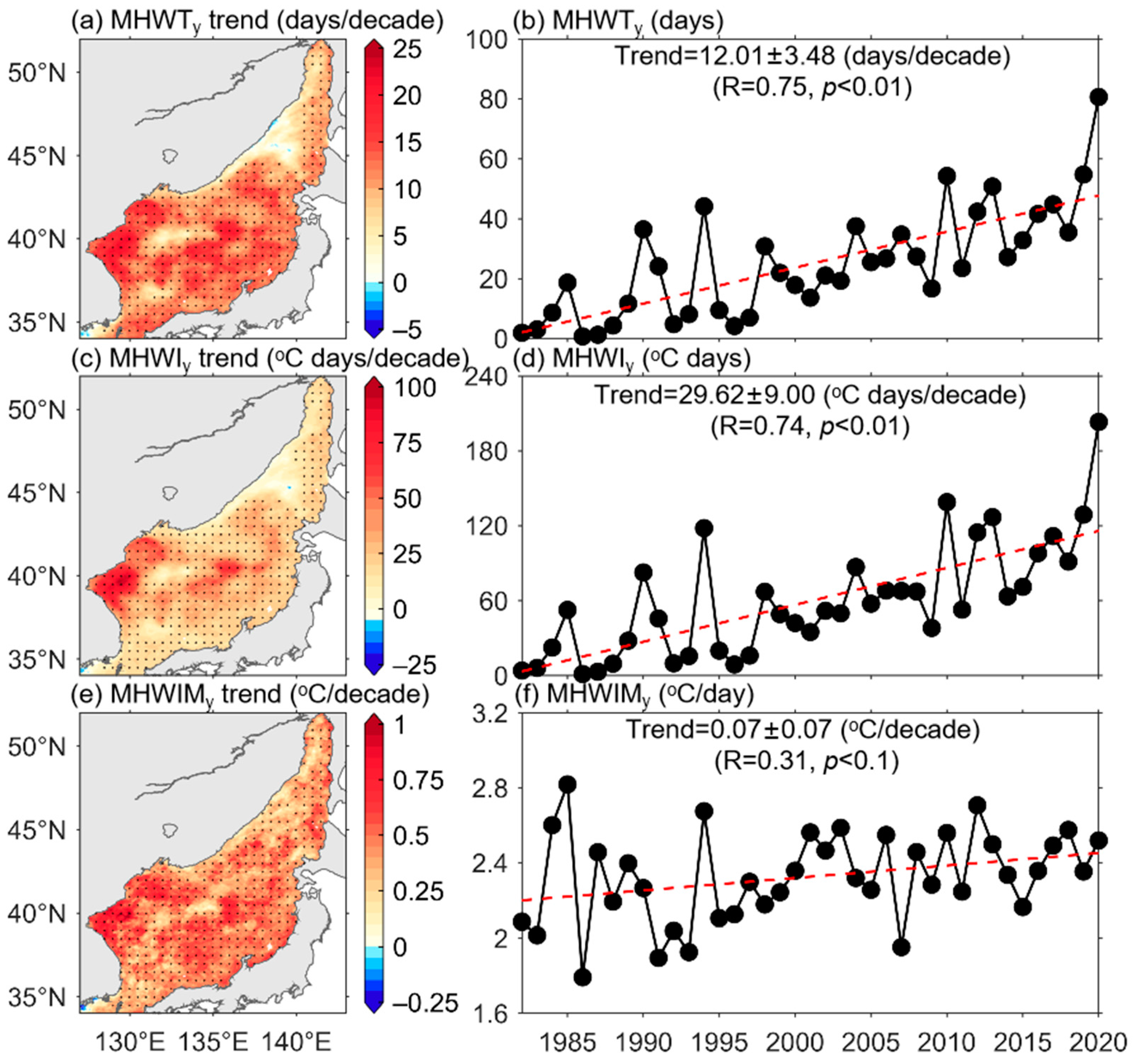
(3)

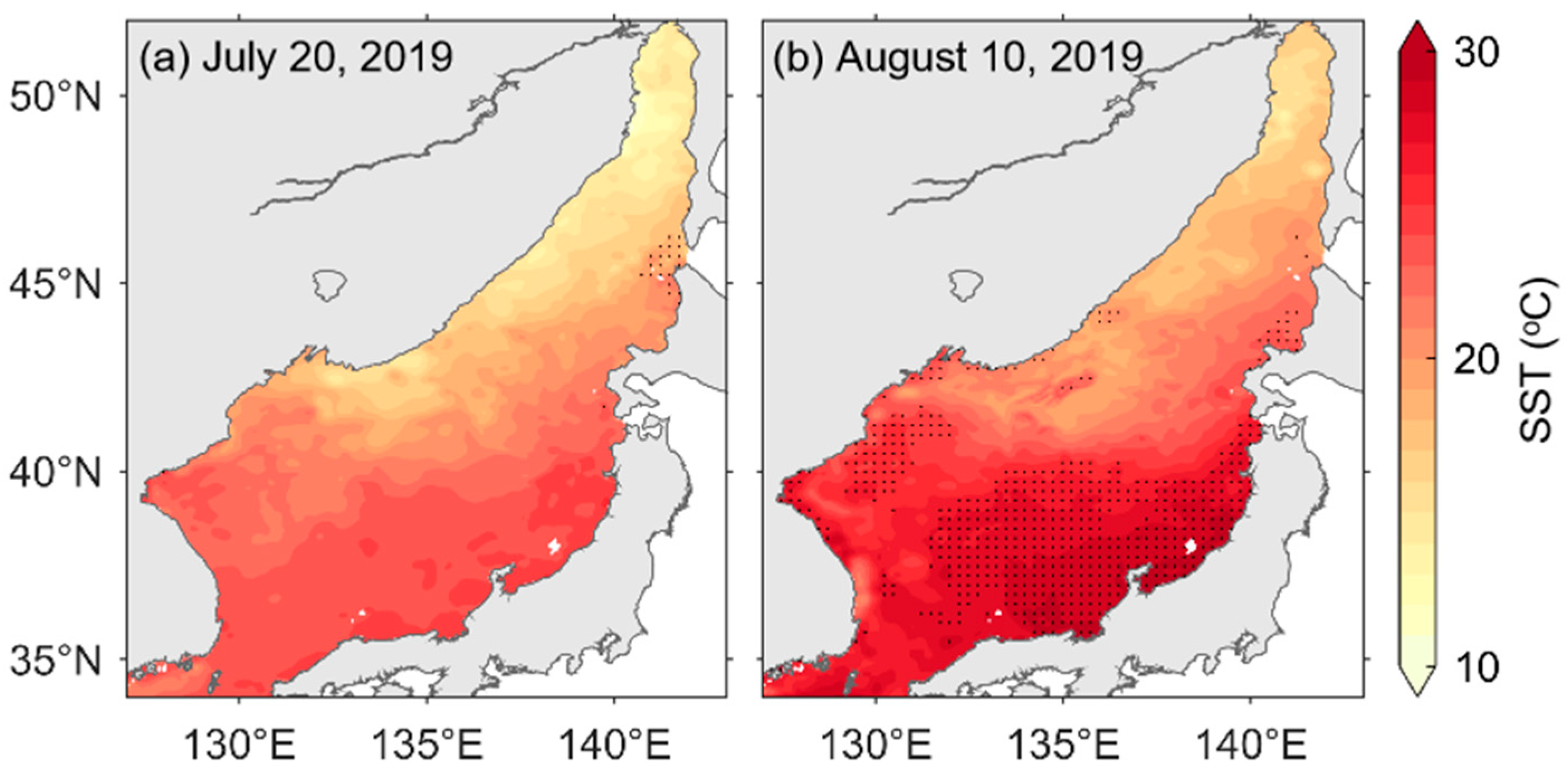
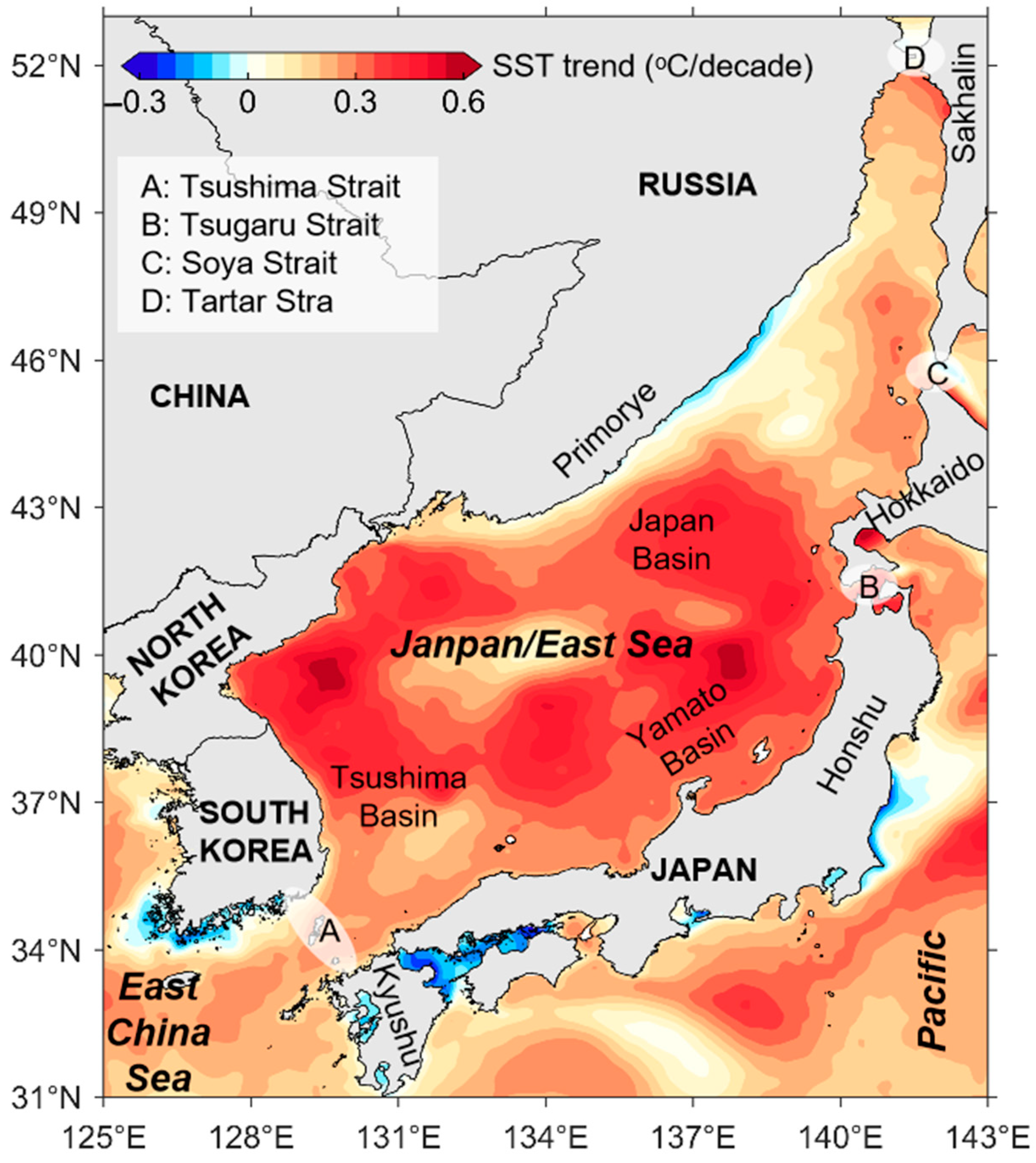
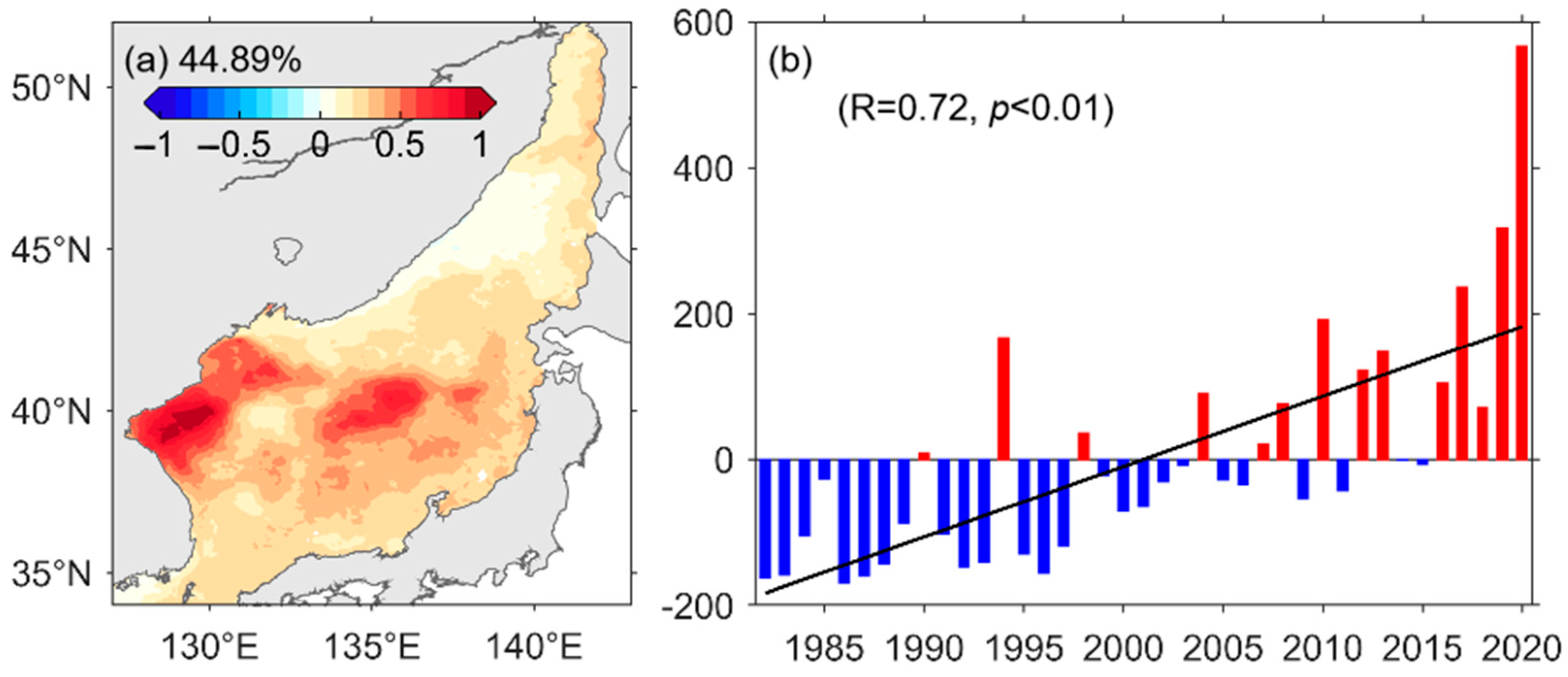
The MHWT_y and MHWI_y have increased significantly in recent years over the entire JES, except for the Russian coastal regions and the Tsushima Strait. Significantly positive trends were observed in the MHWT_y (12.01 ± 3.48 days/decade) and the MHWI_y (29.62 ± 9.00 °C days/decade), which are still significant when the global averaged SST trend is removed. A prolonged MHW event in the western JES lasting more than 200 days (from August 2019 to spring of 2020) is an example of this increasing trend. The increasing trend in the MHWIM_y (0.07 ± 0.07 °C/decade) is rather trivial. The EOF1 of the MHWI_y accounts for 44.89% of the total variance. The corresponding time coefficient shows a significantly increasing trend.

(4)

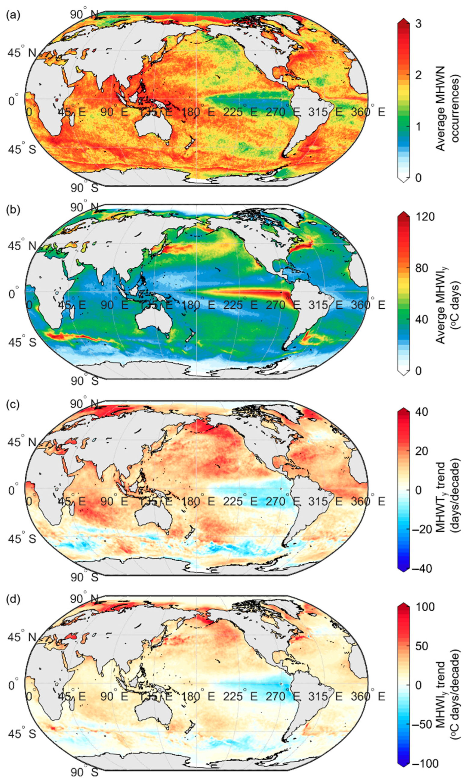
The average JES MHWN was 1.97 occurrences, which is slightly higher than the global average level of 1.82 occurrences. However, regional comparison results indicate that the increasing trend of the MHWI_y in the JES is twice that of the global averaged MHWI trend of 12.37 °C days/decade.

References

1. Hobday, A.J.; Alexander, L.V.; Perkins, S.E.; Smale, D.A.; Straub, S.C.; Oliver, E.; Benthuysen, J.A.; Burrows, M.T.; Donat, M.G.; Peng, M.; et al. A hierarchical approach to defining marine heatwaves. Prog. Oceanogr. 2016, 141, 227–238. [Google Scholar] [CrossRef] [Green Version]
2. Sparnocchia, S.; Schiano, M.E.; Picco, P.; Cappellrtti, A. The anomalous warming of summer 2003 in the surface layer of the Central Ligurian Sea (Western Mediterranean). Ann. Geophys. 2006, 24, 443–452. [Google Scholar] [CrossRef]
3. Garrabou, J.; Coma, R.; Bensoussan, N.; Bally, M.; Chevaldonné, P.; Cigliano, M.; Diaz, D.; Harmelin, J.G.; Gambi, M.C.; Kersting, D.K.; et al. Mass mortality in northwestern mediterranean rocky benthic communities: Effects of the 2003 heat wave. Glob. Chang. Biol. 2009, 15, 1090–1103. [Google Scholar] [CrossRef]
4. Frölicher, T.L.; Laufkötter, C. Emerging risks from marine heat waves. Nat. Commun. 2018, 9, 650. [Google Scholar] [CrossRef] [PubMed]
5. Scannell, H.A.; Pershing, A.J.; Alexander, M.A.; Thomas, A.C.; Mills, K.E. Frequency of marine heatwaves in the North Atlantic and North Pacific since 1950. Geophys. Res. Lett. 2016, 43, 2069–2076. [Google Scholar] [CrossRef] [Green Version]
6. FröLicher, T.L.; Fischer, E.M.; Gruber, N. Marine heatwaves under global warming. Nature 2018, 560, 360–364. [Google Scholar] [CrossRef]
7. Bond, N.A.; Cronin, M.F.; Freeland, H.; Mantua, N. Causes and impacts of the 2014 warm anomaly in the NE Pacific. Geophys. Res. Lett. 2015, 42, 3414–3420. [Google Scholar] [CrossRef]
8. Di Lorenzo, E.; Mantua, N. Multi-year persistence of the 2014/15 North Pacific marine heatwave. Nat. Clim. Chang. 2016, 6, 1042–1048. [Google Scholar] [CrossRef]
9. Chen, W.; Lu, R.; Dong, B. Intensified anticyclonic anomaly over the western North Pacific during El Niño decaying summer under a weakened Atlantic thermohaline circulation. J. Geophys. Res. Atmos. 2014, 119, 13637–13650. [Google Scholar] [CrossRef] [Green Version]
10. Rodrigues, R.R.; Taschetto, A.S.; Gupta, A.S.; Foltz, G.R. Common cause for severe droughts in South America and marine heatwaves in the South Atlantic. Nat. Geosci. 2019, 12, 620–626. [Google Scholar] [CrossRef]
11. Pearce, A.; Lenanton, R.; Jackson, G.; Moore, J.; Feng, M.; Gaughan, D. The “Marine Heat Wave” Off Western Australia during the Summer of 2010/11; Fisheries Research Report No. 222; Department of Fisheries: Perth, Australia, 2011; 40p.
12. Benthuysen, J.A.; Oliver, E.C.; Feng, M.; Marshall, A.G. Extreme marine warming across tropical Australia during austral summer 2015–2016. J. Geophys. Res. Ocean. 2018, 123, 1301–1326. [Google Scholar] [CrossRef]
13. Darmaraki, S.; Somot, S.; Sevault, F.; Nabat, P. Past variability of Mediterranean Sea marine heatwaves. Geophys. Res. Lett. 2019, 46, 9813–9823. [Google Scholar] [CrossRef] [Green Version]
14. Carvalho, K.S.; Smith, T.E.; Wang, S. Bering Sea marine heatwaves: Patterns, trends and connections with the Arctic. J. Hydrol. 2021, 600, 126462. [Google Scholar] [CrossRef]
15. Li, Y.; Ren, G.; Wang, Q.; You, Q. More extreme marine heatwaves in the China Seas during the global warming hiatus. Environ. Res. Lett. 2019, 14, 104010. [Google Scholar] [CrossRef]
16. Gao, G.; Marin, M.; Feng, M.; Yin, B.; Yang, D.; Feng, X.; Ding, Y.; Song, D. Drivers of marine heatwaves in the East China Sea and the South Yellow Sea in three consecutive summers during 2016–2018. J. Geophys. Res. Ocean. 2020, 125, e2020JC016518. [Google Scholar] [CrossRef]
17. Yao, Y.; Wang, J.; Yin, J.; Zou, X. Marine heatwaves in China’s marginal seas and adjacent offshore waters: Past, Present, and Future. J. Geophys. Res. Ocean. 2020, 125, e2019JC015801. [Google Scholar] [CrossRef]
18. Yao, Y.; Wang, C. Variations in summer marine heatwaves in the South China Sea. J. Geophys. Res. Ocean. 2021, 126, e2021JC017792. [Google Scholar] [CrossRef]
19. Oliver, E.C.; Benthuysen, J.C.; Bindoff, N.L.; Hobday, A.J.; Holbrook, N.J.; Mundy, C.N.; Perkins-Kirkpatrick, S.E. The unprecedented 2015/16 Tasman Sea marine heatwave. Nat. Commun. 2017, 8, 16101. [Google Scholar] [CrossRef] [Green Version]
20. Oliver, E.; Lago, V.; Hobday, A.J.; Holbrook, N.J.; Ling, S.D.; Mundy, C.N. Marine heatwaves off eastern Tasmania: Trends, interannual variability, and predictability. Prog. Oceanogr. 2018, 161, 116–130. [Google Scholar] [CrossRef]
21. Salinger, M.J.; Renwick, J.; Behrens, E.; Mullan, A.B.; Diamond, H.J.; Sirguey, P.; Smith, R.O.; Trought, M.C.T.; Alexander, V.L.; Cullen, N.J.; et al. The unprecedented coupled ocean-atmosphere summer heatwave in the New Zealand region 2017/18: Drivers, mechanisms and impacts. Environ. Res. Lett. 2019, 14, 044023. [Google Scholar] [CrossRef]
22. Gentemann, C.L.; Fewings, M.R.; García-Reyes, M. Satellite sea surface temperatures along the West Coast of the United States during the 2014–2016 northeast Pacific marine heat wave. Geophys. Res. Lett. 2017, 44, 312–319. [Google Scholar] [CrossRef]
23. Manta, G.; de Mello, S.; Trinchin, R.; Badagian, J.; Barreiro, M. The 2017 Record Marine Heatwave in the Southwestern Atlantic Shelf. Geophys. Res. Lett. 2018, 45, 12449–12456. [Google Scholar] [CrossRef]
24. Hughes, T.P.; Kerry, J.T.; Álvarez-Noriega, M.; Álvarez-Romero, J.G.; Anderson, K.D.; Baird, A.H.; Babcock, R.C.; Beger, M.; Bellwood, D.R.; Berkelmans, R.; et al. Global warming and recurrent mass bleaching of corals. Nature 2017, 543, 373–377. [Google Scholar] [CrossRef] [PubMed]
25. Smale, D.A.; Wernberg, T.; Oliver, E.C.; Thomsen, M.; Harvey, B.P.; Straub, S.C.; Burrows, M.T.; Alexander, L.V.; Benthuysen, J.A.; Donat, M.G.; et al. Marine heatwaves threaten global biodiversity and the provision of ecosystem services. Nat. Clim. Chang. 2019, 9, 306–312. [Google Scholar] [CrossRef] [Green Version]
26. Benthuysen, J.A.; Oliver, E.C.; Chen, K.; Wernberg, T. Advances in understanding marine heatwaves and their impacts. Front. Mar. Sci. 2020, 7, 147. [Google Scholar] [CrossRef] [Green Version]
27. Hu, S. Observed strong subsurface marine heatwaves in the tropical western Pacific Ocean. Environ. Res. Lett. 2021, 16, 104024. [Google Scholar] [CrossRef]
28. Caputi, N.; Kangas, M.; Denham, A.; Feng, M.; Pearce, A.; Hetzel, Y.; Chandrapavan, A. Management adaptation of invertebrate fisheries to an extreme marine heat wave event at a global warming hot spot. Ecol. Evol. 2016, 6, 3583–3593. [Google Scholar] [CrossRef]
29. Mills, K.E.; Pershing, A.J.; Brown, C.J.; Chen, Y.; Chiang, F.-S.; Holland, D.S.; Lehuta, S.; Nye, J.A.; Sun, J.C.; Thomas, A.C.; et al. Fisheries management in a changing climate: Lessons from the 2012 ocean heat wave in the Northwest Atlantic. Oceanography 2013, 26, 191–195. [Google Scholar] [CrossRef] [Green Version]
30. Seager, R.; Hoerling, M.; Schubert, S.; Wang, H.; Lyon, B.; Kumar, A.; Nakamura, J.; Henderson, N. Causes of the 2011–2014 California drought. J. Clim. 2015, 28, 6997–7024. [Google Scholar] [CrossRef]
31. Cheng, L.; Abraham, J.; Hausfather, Z.; Trenberth, K.E. How fast are the oceans warming? Science 2019, 363, 128–129. [Google Scholar] [CrossRef]
32. Plecha, S.M.; Soares, P.M.M. Global marine heatwave events using the new CMIP6 multi-model ensemble: From shortcomings in present climate to future projections. Environ. Res. Lett. 2020, 15, 124058. [Google Scholar] [CrossRef]
33. Oliver, E.C.; Donat, M.G.; Burrows, M.T.; Moore, P.J.; Smale, D.A.; Alexander, L.V.; Benthuysen, J.A.; Feng, M.; Gupta, A.S.; Hobday, A.J.; et al. Longer and more frequent marine heatwaves over the past century. Nat. Commun. 2018, 9, 1324. [Google Scholar] [CrossRef] [PubMed]
34. Good, S.; Fiedler, E.; Mao, C.; Martin, M.J.; Maycock, A.; Reid, R.; Roberts-Jones, J.; Searle, T.; Waters, J.; While, J.; et al. The Current Configuration of the OSTIA System for Operational Production of Foundation Sea Surface Temperature and Ice Concentration Analyses. Remote Sens. 2020, 12, 720. [Google Scholar] [CrossRef] [Green Version]
35. Hersbach, H.; Dee, D. ERA5 reanalysis is in production. In ECMWF Newsletter; European Centre for Medium-Range Weather Forecasts: Reading, UK, 2016; Volume 147. [Google Scholar]
36. Trouet, V.; Van Oldenborgh, G.J. KNMI Climate Explorer: A Web-Based Research Tool for High-Resolution Paleoclimatology. Tree-Ring Res. 2013, 69, 3–13. [Google Scholar] [CrossRef] [Green Version]
37. Greene, C.A.; Thirumalai, K.; Kearney, K.A.; Delgado, J.M.; Schwanghart, W.; Wolfenbarger, N.S.; Thyng, K.M.; Gwyther, D.E.; Gardner, A.S.; Blankenship, D.D. The Climate Data Toolbox for MATLAB. Geochem. Geophys. Geosyst. 2019, 20, 3774–3781. [Google Scholar] [CrossRef] [Green Version]
38. Amaya, D.J.; Alexander, M.A.; Capotondi, A.; Deser, C.; Karnauskas, K.B.; Miller, A.J.; Mantua, N.J. Are long-term changes in mixed layer depth influencing North Pacific marine heatwaves? Bull. Am. Meteorol. Soc. 2021, 102, S59–S66. [Google Scholar] [CrossRef]
39. Feng, M.; Mcphaden, M.J.; Xie, S.; Hafner, J. La Niña forces unprecedented Leeuwin Current warming in 2011. Sci. Rep. 2013, 3, 1277. [Google Scholar] [CrossRef] [PubMed] [Green Version]
40. Holbrook, N.J.; Scannell, H.A.; Gupta, A.S.; Benthuysen, J.A.; Feng, M.; Oliver, E.C.; Alexander, L.V.; Burrows, M.T.; Donat, M.G.; Hobday, A.J.; et al. A global assessment of marine heatwaves and their drivers. Nat. Commun. 2019, 10, 2624. [Google Scholar] [CrossRef]
41. Qin, H.; Kawamura, H. Surface Heat Fluxes during Hot Events. J. Oceanogr. 2009, 65, 605–613. [Google Scholar] [CrossRef]
42. Gordon, A.L.; Giulivi, C.F. Pacific decadal oscillation and sea level in the Japan/East sea. Deep-Sea Res. I 2004, 51, 653–663. [Google Scholar] [CrossRef]
43. Andres, M.; Park, J.; Mark, W.; Zhu, X.; Nakamura, H.; Kim, K.; Chang, K. Manifestation of the Pacific Decadal Oscillation in the Kuroshio. Geophys. Res. Lett. 2009, 36, L16602. [Google Scholar] [CrossRef] [Green Version]
44. Matsumura, S.; Horinouchi, T. Pacific Ocean decadal forcing of long-term changes in the western Pacific subtropical high. Sci. Rep. 2016, 6, 37765. [Google Scholar] [CrossRef] [PubMed]
45. Gong, D.; Wang, S.; Zhu, J. East Asian winter monsoon and Arctic Oscillation. Geophys. Res. Lett. 2001, 28, 2073–2076. [Google Scholar] [CrossRef]
46. Wu, B.; Wang, J. Winter Arctic Oscillation, Siberian high and East Asian winter monsoon. Geophys. Res. Lett. 2002, 29, 1897. [Google Scholar] [CrossRef]
47. He, S. Reduction of the East Asian winter monsoon interannual variability after the mid-1980s and possible cause. Chin. Sci. Bull. 2013, 58, 1331–1338. [Google Scholar] [CrossRef] [Green Version]
48. Minato, S.; Kimura, R. Volume Transport of the Western Boundary Current Penetrating into a Marginal Sea. J. Oceanogr. Soc. Jpn. 1980, 36, 185–195. [Google Scholar] [CrossRef]
49. Kida, S.; Qiu, B.; Yang, J.; Lin, X. The annual cycle of the Japan Sea Throughflow. J. Phys. Oceanogr. 2016, 46, 23–39. [Google Scholar] [CrossRef]
50. Kida, S.; Takayama, K.; Sasaki, Y.N.; Matsuura, H.; Hirose, N. Increasing trend in Japan Sea Throughfow transport. J. Oceanogr. 2021, 77, 145–153. [Google Scholar] [CrossRef]
51. Wie, J.; Moon, B.; Hyun, Y.; Lee, J. Impact of local atmospheric circulation and sea surface temperature of the East Sea (Sea of Japan) on heat waves over the Korean Peninsula. Theor. Appl. Climatol. 2021, 144, 431–446. [Google Scholar] [CrossRef]
52. Jung, S. Asynchronous responses of fish assemblages of climate-driven ocean regime shifts between the upper and deep layer in the Ulleung Basin of the East Sea from 1986 to 2010. Ocean Sci. J. 2014, 49, 1–10. [Google Scholar] [CrossRef]
Figure 1. Sea surface temperature (SST) trend in the Japan/East Sea (JES). The Tsushima, Tsugaru, Soya, and Tartar Straits are marked as A, B, C, and D on the map, respectively.
Remotesensing 14 00936 g001
Figure 2. Sea surface temperature (SST) distribution on 20 July 2019 (a) and 10 August 2019 (b). The point grid indicates an occurring marine heatwave (MHW).
Remotesensing 14 00936 g002
Figure 3. Schematic of metrics used to define marine heatwaves (MHWs) at any grid point. (a) 11-day window centered on calendar day d of year y; (b) climatological mean (blue dash) and 90th percentile threshold value (green dash) for day j of the year; (c) unsmoothed climatological mean (Tclm, pink line) and 31-day smoothed climatological mean (Tm, blue line); (d) MHWs (red shading) detected in year y, exceeding the 31-day smoothed threshold (green line) and lasting for at least 5 days. The start and end days of the MHW are represented by ts and te, respectively. T ( t s t t e ) > T s , where T is the daily SST and t is the time.
Remotesensing 14 00936 g003
Figure 4. Spatial distribution of marine heatwave (MHW) indices from 1982 to 2020. (a) Average number of MHWs (MHWN); (b) average yearly sum of MHW-day (MHWTy); (c) mean duration of MHWs (MHWD); (d) mean MHW maximum intensity (Imax), and (e) mean MHW mean intensity (Imean).
Remotesensing 14 00936 g004
Figure 5. Probability density function (PDF) distribution of mean intensity (Imean) and duration (MHWD) of marine heatwaves (MHWs) in the Japan/East Sea (JES) from 1982 to 2020. The resolutions for MHWD and Imean are 1 day and 0.1 °C, respectively.
Remotesensing 14 00936 g005
Figure 6. Spatial distribution of average monthly sum of MHW-day (MHWTm) in the Japan/East Sea (JES) from 1982 to 2020. The subfigures (al) are from January to December, respectively.
Remotesensing 14 00936 g006
Figure 7. Spatial distribution of average monthly mean MHW-intensity (MHWIMm) in the Japan/East Sea (JES) from 1982 to 2020. The subfigures (al) are from January to December, respectively.
Remotesensing 14 00936 g007
Figure 8. Spatial distribution of average monthly sum of MHW-intensity (MHWIm) in the Japan/East Sea (JES) from 1982 to 2020. The subfigures (al) are from January to December, respectively.
Remotesensing 14 00936 g008
Figure 9. Area-averaged marine heatwave (MHW) indices in the Japan/East Sea (JES) from 1982 to 2020. (a) Monthly sum of MHW-day (MHWTm); (b) monthly sum of MHW-intensity (MHWIm); (c) monthly mean MHW-intensity (MHWIMm).
Remotesensing 14 00936 g009
Figure 10. Area-averaged marine heatwave (MHW) indices in the Japan/East Sea (JES) from 1982 to 2020. (a) Monthly sum of MHW-day (MHWTm); (b) monthly sum of MHW-intensity (MHWIm); (c) monthly mean MHW-intensity (MHWIMm).
Remotesensing 14 00936 g010
Figure 11. Variations of marine heatwave (MHW) indices in the Japan/East Sea (JES) from 1982 to 2020. (a) Trends in yearly sum of MHW-day (MHWTy); (b) annual area-averaged MHWTy; (c) trends in yearly sum of MHW-intensity (MHWIy); (d) annual area-averaged MHWIy; (e) trends in yearly mean MHW-intensity (MHWIMy); (f) annual area-averaged MHWIMy. The stippled areas indicate significant trends where p-values are less than 0.05. Dashed red lines represent the linear trends of regionally averaged MHW indices.
Remotesensing 14 00936 g011
Figure 12. Empirical orthogonal function (EOF) analysis of the yearly sum of MHW-intensity (MHWIy) in the Japan/East Sea (JES) from 1982 to 2020. (a) Spatial pattern of the first EOF mode (EOF1); (b) time coefficients of the EOF1 (PC1).
Remotesensing 14 00936 g012
Figure 13. (a) Time series of normalized time coefficients of the first empirical orthogonal function mode (PC1), area-averaged sea surface temperature anomaly (SSTA), Pacific Decadal Oscillation (PDO) index, Arctic Oscillation (AO) index, and Niño index; average yearly sum of MHW-day (MHWTy) of (b) positive PDO years, (c) positive AO years, (d) positive Niño years, (e) negative PDO years, (f) negative PDO years, and (g) negative Niño years.
Remotesensing 14 00936 g013
Figure 14. Variations of factors from 1982 to 2020. (a) Trends in net surface heat flux (SHF); (b) annual area-averaged SHF; (c) trends in freshwater flux (SWF); (d) annual area-averaged SWF; (e) trends in 10-m wind speed; (f) annual area-averaged 10-m wind speed; (g) trends in Ekman pumping vertical velocity ( w E ); (h) annual area-averaged w E . The stippled areas indicate significant trends where p-values are less than 0.05. Dashed red lines represent the linear trends of regionally averaged MHW indices.
Remotesensing 14 00936 g014
Figure 15. Variations of factors from 1982 to 2020. (a) Trends in surface net solar radiation (SSR); (b) annual area-averaged SSR; (c) trends in surface net thermal radiation (STR); (d) annual area-averaged STR; (e) trends in surface sensible heat flux (SSHF); (f) annual area-averaged SSHF; (g) trends in surface latent heat flux (SLHF); (h) annual area-averaged SLHF. The SSR, STR, SSHF, and SLHF with downward direction are set to be positive. The stippled areas indicate significant trends where p-values are less than 0.05. Dashed red lines represent the linear trends of regionally averaged MHW indices.
Remotesensing 14 00936 g015
Figure 16. Spatial pattern of the correlation coefficient between the first empirical orthogonal function mode (PC1) and variables associated with marine heatwaves. (a) Net surface heat flux (SHF); (b) surface net solar radiation (SSR); (c) surface net thermal radiation (STR); (d) surface sensible heat flux (SSHF); (e) surface latent heat flux (SLHF); (f) freshwater flux (SWF); (g) evaporation (E); (h) total precipitation (P); (i) 10-m wind speed; (j) Ekman pumping vertical velocity ( w E ); (k) significant height of wind waves (SWH); (l) significant height of total swell (SHTS). The stippled areas indicate significant correlations where p-values are less than 0.05.
Remotesensing 14 00936 g016
Figure 17. Mean states and trends of global marine heatwave (MHW) indices from 1982 to 2020. (a) Average number of MHWs (MHWN); (b) average yearly sum of MHW-intensity (MHWIy); (c) trends in yearly sum of MHW-day (MHWTy); (d) trends in MHWIy.
Remotesensing 14 00936 g017