Abstract
Deep-learning methods rely on massive labeled data, which has become one of the main impediments in hyperspectral image change detection (HSI-CD). To resolve this problem, pseudo-labels generated by traditional methods are widely used to drive model learning. In this paper, we propose a mutual teaching approach with momentum correction for unsupervised HSI-CD to cope with noise in pseudo-labels, which is harmful for model training. First, we adopt two structurally identical models simultaneously, allowing them to select high-confidence samples for each other to suppress self-confidence bias, and continuously update pseudo-labels during iterations to fine-tune the models. Furthermore, a new group confidence-based sample filtering method is designed to obtain reliable training samples for HSI. This method considers both the quality and diversity of the selected samples by determining the confidence of each group instead of single instances. Finally, to better extract the spatial–temporal spectral features of bitemporal HSIs, a 3D convolutional neural network (3DCNN) is designed as an HSI-CD classifier and the basic network of our framework. Due to mutual teaching and dynamic label learning, pseudo-labels can be continuously updated and refined in iterations, and thus, the proposed method can achieve a better performance compared with those with fixed pseudo-labels. Experimental results on several HSI datasets demonstrate the effectiveness of our method.
1. Introduction
Hyperspectral imaging techniques can obtain continuous spectral information over a wide range of spectral wavelengths. The ability to display the subtle spectral variations of different ground objects has played an important role in many land-cover monitoring applications, such as mineral exploration [,], land-use monitoring [,], and military defense []. Change detection (CD) is the process of identifying differences in the state of an object or phenomenon by observing it at different times [], which has been an indispensable application in the remote sensing field for a long time. Because of the rapid increase in spectral information, hyperspectral images (HSIs) are able to help detect finer changes than other remote sensing images and observe more change details. However, due to the spectral variability and redundant information, it is still a substantial challenge to effectively mine the spectral–spatial information to complete the HSI-CD task.
For decades, a variety of unsupervised methods have been applied to HSI-CD. Change detection aims to generate an accurate binary change map. In traditional methods, the change map can be obtained by analyzing the difference image (DI), which is usually based on differencing or log-rationing function. The most typical method is the change vector analysis (CVA) method [], which identifies the changed pixels and the type of change according to the magnitude and direction of the spectral change vector. Some techniques utilize image transformation to extract new features for better performance. Principal component analysis (PCA) [] retains the main information of original images according to the statistical characteristics, which reduces data redundancy enormously. Both multivariate alteration detection (MAD) [] and the improved iteratively reweighted MAD (IRMAD) [] methods calculate the degree of change by canonical correlation analysis. These measures all assume that the characteristics of unchanged pixels are uniform, but in reality, due to atmospheric conditions, illumination, etc., completely identical features rarely exist []. To suppress the difference in unchanged pixels, slow feature analysis (SFA) extracts the most temporally invariant component and then converts images into a new feature space []. Furthermore, some methods [,] directly determine the changing type of pixels using the postclassification comparison (PCC), but their performances fully depend on the accuracy of the classifier.
Recently, deep-learning (DL) methods have been favored by many researchers because of their strong nonlinear representation ability. Change detection needs to process bitemporal images simultaneously, as feature fusion must be carried out to form a single feature vector, which is usually a similarity measure between those two features []. Conventional methods inevitably lose partial information via difference or other processing, while deep-learning methods can avoid this problem. Mou et al. [] proposed an end-to-end network. A convolutional neural network (CNN) extracts spectral–spatial features and a recurrent neural network (RNN) analyzes the temporal dependence between images. Considering the mixed pixels in HSIs, some methods [] utilize subpixel-level information obtained by unmixing to improve detection accuracy. Chen et al. [] proved that the 3D convolution kernel combined with regularization can effectively extract the spectral–spatial features of HSIs for classification tasks. Based on this, a 3D convolutional neural network (3DCNN) for hyperspectral image change detection is designed as the basic model of the proposed framework.
However, the great success of existing deep learning methods in many tasks mainly benefits from a large amount of labeled data. Pixel-wise labels for bitemporal HSIs need to be annotated by experts, which is time-consuming and expensive. Thus, it is difficult to obtain in large quantities. To solve the problem, existing unsupervised HSI-CD methods usually use pseudo-labels generated by traditional algorithms [,,,]. One of the main challenges is that the training process of neural networks is susceptible to noise in pseudo-labels. It is difficult to deal with the high-dimensionality of hyperspectral data for traditional CD methods. Additionally, affected by atmospheric conditions, illumination, and topography changes, the spectral variability of ground objects further increases the difficulty of change detection. Due to the limitations of these traditional methods, there certainly exist some discrepancies between the pseudo-labels and the true labels. Zhang et al. [] proved that advanced neural networks can easily fit training sets with arbitrary labels. Once the network fits inaccurate labels, it will seriously affect the classification results. Wang et al. [] utilized subpixel information to enhance robustness of the model. Du et al. [] designed a deep slow feature analysis (DSFA) algorithm based on SFA theory and deep network to extract invariant components. These methods largely ignore handling the noisy labels. Li et al. [] added a noisy model with zero-mean Gaussian distribution to their loss function, yet the experimental effect was general. The authors in [] adopted two unsupervised algorithms to jointly generate credible labels. However, the same problem still exists, where it is impossible to filter all noisy labels by only one-time sample selection.
To address the noisy labels, we propose dynamically correcting pseudo-labels instead of safely relying on labels. The momentum correction approach is based on mutual teaching, where two learning models are mutually updated to jointly learn. Dynamic learning approaches by sample selection are popular in robust learning from noisy labels [,,,,]. Yao et al. [] adjusted the number of training samples in each iteration according to the learning curve. Self-paced learning (SPL) [,], which reduces the confidence threshold as the number of iterations increases, automatically selects more complex samples. However, the self-training of networks is prone to self-confidence bias and cannot be corrected when errors accumulate. Co-teaching [] trains two classifiers simultaneously and enables them to select small loss samples for each other in every mini-batch, effectively suppressing the phenomenon of overfitting. It is generally assumed that small loss samples are more likely to be correctly labeled. Nevertheless, simply using loss to select training data is not suitable for bitemporal HSIs with complex variations. The selected samples are easily concentrated in the two categories of maximum and minimum changes, which is not conducive to the generalization of models. Therefore, we divide all samples into multiple groups according to the similarity of the difference vector in advance and randomly select from the high-confidence groups to ensure that multiclass samples can be selected. In addition, although our approach uses incompletely correct labels during initialization, utilizing the newly derived more reliable results to update the pseudo-labels can further boost the classifier performance [,]. The main contributions are summarized as follows:
- (1)
- We introduce to a novel mutual teaching framework with momentum correction for resisting noisy labels generated by traditional methods in unsupervised HSI-CD. Due to mutual teaching and dynamic label learning, pseudo-labels can be continuously updated and refined in iterations, and thus the proposed method can achieve superior results.
- (2)
- A group confidence-based sample selection approach is proposed to avoid selecting the two most extreme types of samples, and it is used alternately with another selection mechanism in iteration to ensure that complex samples can participate in training.
- (3)
- An end-to-end 3DCNN is designed as a classifier for HSI-CD and the basic model of the proposed framework. Experiments on four datasets demonstrate that our framework can effectively improve model performance.
2. Related Work
2.1. Unsupervised Deep Methods for Change Detection
Remote sensing image annotation is more difficult than that of natural images, especially for pixel-level change detection. Therefore, unsupervised methods without manual labeling steps have more advantages. Currently, unsupervised deep-learning methods can be divided into two categories. As shown in Figure 1a, the network is treated as a feature extractor to transform original images into a new feature space, and the model parameters are optimized based on the analysis of current output features in each iteration. For example, Liu et al. [] proposed a symmetric convolutional coupling network (SCCN), which was initialized by a denoising autoencoder, and then minimized the feature difference between those unchanged pixels. Zhang et al. [] adopted clustering analysis and detected multiple types of changes. Liu et al. [] established an energy function driven network according to the feature difference. The advantage of these methods is that the newly derived features are used in each iteration to progressively improve the accuracy of the results. However, due to the limitation of optimization, it is difficult to use more complex models without any labels and the high dimension of HSIs is not conducive to model convergence. The other is shown in Figure 1b. The results obtained by the traditional algorithms are assigned to all samples as pseudo-labels to train neural networks, which is more commonly used [,,,,,,,]. These methods are easy to implement and closer to end-to-end patterns, avoiding the intermediate steps of difference image analysis. The only problem is that the pseudo-labels are not completely correct, which may mislead the network training. Inspired by the first category of methods, we utilize new predictive values to update pseudo-labels in multiple iterations to gradually reduce noise labels.
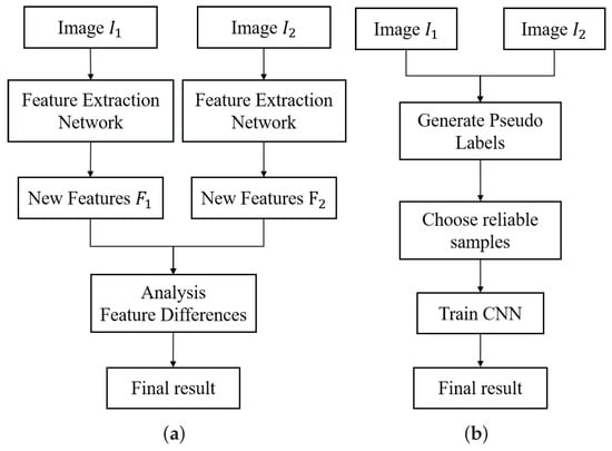
Figure 1.
Architectures of two unsupervised deep methods for change detection. (a) Feature analysis-driven model training. (b) Pseudo-labels-driven model training.
2.2. Deep Learning with Noisy Labels
Noisy labels are ubiquitous in deep-learning applications, such as in large-scale low-quality datasets collected from the internet or crowdsourcing platforms in supervised learning, predictive pseudo-labels in semi-supervised learning and in domain adaptation learning. The overfitting of noisy labels will directly weaken the generalization of the models. Thus, learning with noisy labels still attracts researchers’ attention. The noise transition matrix and robust loss function are commonly used for antinoise training. Goldberger et al. [] added another softmax layer to capture the transitional relationship between the noisy and true labels. Ghosh et al. [] confirmed that the loss function based on the mean-absolute error is inherently robust to noise. CleanNet [] determined whether the sample label is correct by comparing it with a representative “class prototype”. However, these methods generally require prior knowledge or rely on certain constraints. To avoid consuming additional resources or more complex networks, it is a good way to select clean parts from noisy instances to update models. The memorization effects of deep neural networks show that the samples with smaller values collected from the loss function are more likely to be correctly annotated. Therefore, some studies [,,,] allow the model to select reliable samples for itself in each iteration to improve classification accuracy, which is similar to active learning and reinforcement learning.
2.3. Mutual Teaching Paradigm
Although sample selection can effectively prevent noisy labels from participating in training, it is difficult to ensure that the selected labels are absolutely clean. The self-training process is sensitive to noise and outliers, and multiple iterations will accumulate the model bias caused by a few wrongly selected instances or unbalanced samples. For this purpose, MentorNet [] is learned to compute time-varying weights for each training sample based on a predefined course, which provides meaningful supervision to help StudentNet overcome corrupted labels. However, the problem of error accumulation still exists. Inspired by co-training [], co-teaching [] trains two identical deep networks and lets them select small loss samples for each other in every minibatch. The difference between them is that co-training needs to establish two viewpoints to generate reliable pseudo-labels, which are generally used for semisupervised learning. Co-teaching only needs one viewpoint, which utilizes the randomness of the network training process to resist self-confidence bias, similar to finding their potential shortcomings by “peer-review”. Likewise, deep mutual learning [] enables multiple student networks to learn from each other to produce a more robust and generalized network in model distillation. This simple and effective learning paradigm is easily extended to other applications [,,,]. Unfortunately, few studies have focused on pseudo-label noise in HSI-CD. Therefore, we develop a dynamic change detection framework using the novel mutual teaching approach and an improved sample selection method.
3. Methodology
In this section, we detail the proposed method from three aspects: the training process of the mutual teaching framework, sample selection and class balancing, and the classifier for HSI-CD.
3.1. The Mutual Teaching Framework
An overview of the proposed mutual teaching framework for bitemporal HSI-CD is shown in Figure 2. First, the original pseudo-labels are obtained from a traditional method, and after screening, they are used to initialize two DL models with the same structure. After each iteration, the two DL models update pseudo-labels for each other with new predictions and alternately use two different sample selection procedures to ensure the accuracy and diversity of training instances. In the end, the final result is generated by combining the predictions of the two models.
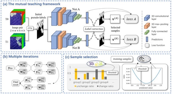
Figure 2.
Graphical illustration of the proposed method. (a) Overall framework of the proposed mutual teaching based on collaborative training and label correction. Both models update their pseudo-labels with each other’s predictions and select clean samples to optimize parameters. (b) The model parameters and pseudo-labels are alternately updated and the final result is generated by the predictions of the two models. (c) Two sample selection methods jointly ensure the accuracy and diversity of training samples.
In this work, the HSI-CD task is regarded as a classification problem, that is, to determine whether the sample corresponding to each pixel belongs to the changed or unchanged class. Taking a pair of pixels in the same position of bitemporal images as a training instance. With a total of m samples, is the ith sample, and m equals , where w and h are the width and height of the original image, respectively. We adopt the CVA algorithm to obtain initial pseudo-labels , equals 1 to represent the change sample, and 0 is unchanged. In contrast to the existing deep-learning-based change detection methods, the pseudo-labels generated by CVA are only used to initialize the parameters of the two networks and and serve as initial values of and . They will be updated dynamically by mutually training the two networks.
To further improve the accuracy of classifiers, it is necessary to select samples with the label as correct as possible. After feeding all pseudo-labels into the sample selection program, two sets of training data and can be obtained. Here indicates whether the sample is selected, where equals 1 indicating selected and 0 unselected. The parameter updating procedures of both models are described below:
where is the loss between the classifier’s predicted value and the pseudo-label . Then, we can update the pseudo-labels with a new prediction:
where is the momentum parameter. Note that both models use each other’s predicted values to update their own pseudo-labels for mutual teaching purposes.
Sample selection can effectively reduce noisy labels, but it is impossible to completely screen them. Due to various factors such as unbalanced samples and noisy labels, it is inevitable for the classifier to generate confidence bias. The error will be transferred back to itself in the next iteration, and it should be increasingly accumulated in the self-training process. Benefiting from the respective training of the two models, they can filter out different types of errors by mutual teaching and effectively reduce the accumulation of these errors. Meanwhile, with the improvement of model prediction accuracy, the influence of noisy labels can also be mitigated by gradually modifying pseudo-labels. After multiple iterations, the final results are derived from the predicted values of two classifiers. When their predictions are different, we choose one with less loss.
3.2. Sample Selection
To reduce the impact of noisy labels, sample selection is utilized in large studies. The most common approach is to judge the credibility according to the sample loss, which can be formulated as:
The threshold is a critical parameter. When is too large, noisy labels will increase, and when is too small, the lack of complex samples is not conducive to the generalization of the classifier.
In previous studies [,], the above selection method was used, and it is designed for synthetic aperture radar (SAR) image data, which is comparatively simple. However, it performs poorly on HSIs. The selected samples tend to focus on the simplest regions and ignore other types. Thus, we need to design a more appropriate sample selection algorithm for such HSIs. Considering the distribution of data, we use a clustering-based method to select data in blocks. The data in the same cluster have high similarity. When most samples in the cluster have consistent prediction, it is relatively reliable. To select samples of different types evenly and ensure correct labels, a group confidence-based sample selection approach is designed, as shown in Figure 3. First, the PCA is used to reduce the feature dimension of the difference image, and k-means algorithm is applied on the results to obtain the grouping information. Then, we can obtain a grouping label vector , which indicates the grouping information of all samples and takes the value in , while n is the total number of groups. We consider the label with the highest proportion in each group as the group label:
where is the pseudo-label; , is the group label. If there are more changed samples than unchanged samples within the group, takes 1; otherwise, it takes 0. The group confidence is determined by the proportion of group labels:
where represents a group confidence vector. When the value exceeds a certain threshold, the sample in the group is considered reliable:
where is the group confidence threshold. Note that we only select samples with the same label as the group. In this way, the selected training dataset contains samples of varying degrees of change and has a low proportion of noisy labels.

Figure 3.
Sample selection based on group confidence. (a) Pseudo-labels. (b) Multiclass map. (c) Sample loss-based method. (d) Group confidence-based method. In (c,d), white is the selected samples with correct label, red is the selected noisy samples, and black is the discarded samples.
Figure 3c,d shows the samples selected in two ways respectively. It is obvious that the dataset contains two main changes, and the changed samples selected by a single sample confidence focus on one class while ignoring the other. Moreover, the sampling of our method is more even, and the noisy labels contained in both methods are negligible. Another advantage of our method is that it can be used on pseudo-labels of discrete values, such as 0 or 1. The sample loss-based algorithm can only be used on continuous values, which are usually between 0 and 1.
The group confidence-based sample selection approach can consider screening noisy labels and the diversity of the training data. There are mainly two kinds of samples to be discarded: one with low group confidence and the other has a different label from most of the samples in the group. Thus, some complex samples may never participate in training, and the two models cannot adequately exchange information. Therefore, we alternately use two selection strategies to jointly guarantee the accuracy and the stability of the final results, as shown in Figure 2c. The group confidence-based sample selection method is used to select samples which are as clean possible, to improve the accuracy of models, and the parameter is set to 0.8. The loss-based method is used to select as many samples as possible to encourage these easily overlooked complex samples to participate in training, and the parameter is set to 0.4.
In addition, we apply different weights for sample loss to balance class. General binary classification uses cross-entropy loss, which can be defined as follows:
where is the predicted value. Then, the final weighted loss function is:
where the first item enhances the weight of large loss samples, and is set to 2 according to article []. The weighted loss can balance the multiclass samples to avoid a large deviation of the model. The entire procedure for the proposed method is summarized in Algorithm 1.
| Algorithm 1: Procedure of the proposed method. |
Input: Two images and ; thresholds and ; the number of iterations ; the momentum parameter . Output: The final result . // Initialization Get pseudo-labels and multiclass map ; initialize and ; Randomly initialize and ; for to do if then Update selected sample and by (6); else Update selected sample and by (3); end Update pseudo-labels and by (2); end , |
3.3. A 3D Convolutional Neural Network Establishment
The bitemporal hyperspectral data have four dimensions, two spatial axes, a spectral axis and a temporal axis. To extract features using general 2D convolution kernels, most change detection methods reduce one dimension of data by stacking or with a difference operation. However, direct stacking increases the number of convolution kernel channels and network parameters, especially for HSIs with hundreds of channels, and the difference operation leads to the loss of original information. In HSI classification, the authors in [] verified that 3D convolution can better extract spectral spatial features of HSI than 2D convolution. In some video processing applications, 3D convolution kernel has been used to extract temporal and spatial features simultaneously. Similar to change detection, these kinds of data have an additional temporal dimension relative to a single image. Therefore, 3D convolution is an appropriate feature extractor without additional operations in HSI-CD.
In convolutional layers, the calculation of new features uses convolution kernels to multiply local domain features of the previous layer, then adds a bias and passes through an activation function. For 2D convolution, the value of the feature map extracted by the ith convolution kernel of the lth layer at position is calculated as:
where is the activation function, and are the height and width of the kernel, is the value of the kernel connected to the feature map at position , m represents the th layer feature map connected to the current feature, and is the bias. For 3D convolution, the value of the feature map extracted by the ith convolution kernel of the lth layer at position is calculated as:
where is the size of the 3D kernal along the spectral dimension. Because the adjacent spectral channels of HSIs have a strong correlation, it is reasonable to extract the spatial and spectral neighborhood information of two images simultaneously with 3D convolution.
For HSI-CD tasks, we design a 3D convolutional neural network as the basis classifier, as shown in Figure 4. A sample consists of two data blocks of a neighborhood size of 3 extracted from bitemporal images at the same location, and is filled to size 5 with 0 when input into the network. After three 3D convolution layers and a pooling layer, the fused feature vector is extracted, and finally, the change information is output through two fully connected layers. The last layer is activated by the softmax function, and the other uses the ReLU function. After all of the samples are fed into the network, a result map with the same size as the original image representing the degree of change can be obtained. To verify the effectiveness of 3D convolution, we design a similar 2D convolutional neural network for comparison in subsequent experiments.
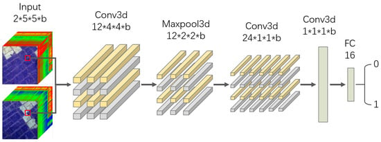
Figure 4.
Architecture of the proposed 3DCNN.
4. Result
To verity the effectiveness of the proposed method, several experiments were conducted using a multispectral dataset and three popular hyperspectral datasets. This section first introduces the datasets used in the experiment. Then the evaluation measures of change detection and experimental setup are described. Finally, comparative experiments with other methods are analyzed in detail.
4.1. Introduction to Datasets
The first dataset “Bastrop” is shown in Figure 5a,b, which consists of two multispectral images (MSI) taken before and after a forest fire in Bastrop County, Texas, in September 2011 and October 2011 []. This multispectral dataset was selected from Landsat 5 Thematic Mapper (TM) multispectral images consisting of six spectral bands with a spatial resolution of 30 m for bands 1–5 and 7 and one thermal band (band 6). Their spatial size is 1534 × 808 pixels with 7 bands.
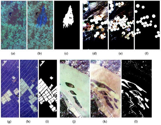
Figure 5.
Experimental datasets. (a) Bastrop dataset in September 2011. (b) Bastrop dataset in October 2011. (d) Umatilla dataset on 1 May 2004. (e) Umatilla dataset on 8 May 2007. (g) Yancheng dataset on 3 May 2006. (h) Yancheng dataset on 23 April 2007. (j) River dataset on 3 May 2013. (k) River dataset on 31 December 2013. (c,f,i,l) groundtruth change map for Bastrop, Umatilla, Yancheng and River dataset, respectively.
The other three HSI datasets were collected from Earth Observing-1 (EO-1) Hyperion data. EO-1 has a spectral resolution of 10 nm and a spatial resolution of approximately 30 m, with a total of 242 different bands. The second dataset “Umatilla” is irrigated farmland in Umatilla County, OR, USA, as shown in Figure 5d,e. The images contain 390 × 200 pixels and 242 bands. The third dataset, “Yancheng”, was acquired on 3 May 2006, and 23 April 2007, in Yancheng, Jiangsu Province, China, as shown in Figure 5g,h. The two images both consist of 450 × 140 pixels with 155 bands after eliminating the noise. The fourth dataset, “river”, was obtained on 3 May 2013, and 31 December 2013, in Jiangsu Province, China, as shown in Figure 5j,k. This dataset contains two HSIs with 463 × 241 pixels and 198 channels [].
4.2. Evaluation Measures and Experimental Configurations
In this paper, specific evaluation metrics are used to evaluate the change detection results of all methods on the datasets. Generally, the results of change detection use pixel-level indicators, which mainly include the following four metrics: true positives (TP), true negatives (TN), false positives (FP), and false negatives (FN). The positive sample refers to the changed samples, displayed in white in the result image, and the negative sample refers to unchanged samples, displayed in black. The correct rate of classification is represented by the overall accuracy (OA), and the formula is
Compared with OA, the kappa coefficient and F1 score can better reflect the consistency between the predicted results and the actual results. It is calculated as
For the experimental setting, the proposed 3DCNN network structure is shown in Figure 4. For hyperspectral images, the size of the first two 3D convolution kernels is , while on the Bastrop dataset, the size of the 3D convolution kernels is because it has only seven bands. The parameter n is the total number of groups. For the Bastrop datasets, n is set to 10, and for the other three datasets, n is set to 20. The momentum parameter is set to 0.4.
4.3. Comparison with Other Methods
To verity the effectiveness of the proposed method, we tested our method on three hyperspectral datasets and a multispectral dataset, then compared it with other classical methods, including the change vector analysis (CVA) [], iteratively reweighted multivariate alteration detection (IRMAD) [], iterative slow feature analysis (ISFA) [], support vector machines (SVM), GETNET [], 2DCNN, and 3DCNN. The Otsu threshold algorithm is used in CVA to generate the final change detection result, which is used as pseudo-labels for other methods that require labeled data. Among the above methods, only CVA, IRMAD and ISFA do not require labeled samples. Other classification-based methods use the same pseudo-labels for supervised training and select training samples through our proposed sample selection method.
4.3.1. Experiments on the Bastrop Dataset
Figure 6 shows the final binary result images of the eight methods, and Table 1 lists the results of the numerical evaluation. It can be clearly seen from the figure that there is a large amount of misclassification noise in CVA, mainly false negative samples, and the kappa coefficient is only . IRMAD is the worst and ISFA is relatively better among the three unsupervised traditional algorithms, but they have the same problems. Other methods use the results of CVA as pseudo-labels to train their models. Although SVM significantly reduces FP values, it also leads to a huge deviation that causes the changed samples to be mistaken for unchanged. Then, the kappa coefficient was reduced by . Deep-learning methods have wonderful advantages. They all increase the OA and the kappa coefficients and outperform traditional algorithms visually. Remarkably, the performance of our method is considerably better than other methods on this dataset, with kappa rising to 0.9406, which is higher than the second-highest value. In particular, a large number of false negative samples have been well-corrected.
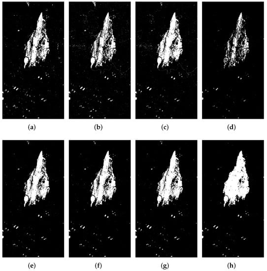
Figure 6.
The change map on Bastrop dataset. (a) CVA. (b) IRMAD. (c) ISFA. (d) SVM. (e) GETNET. (f) 2DCNN. (g) 3DCNN. (h) ours.

Table 1.
Quantitative evaluation of CD results by different methods for Bastrop dataset.
4.3.2. Experiments on the Umatilla Dataset
These dataset results are shown in Figure 7 and listed in Table 2. Among the three unsupervised traditional algorithms, CVA has the most serious noise and the lowest accuracy. From the visual effect, the results of IRMAD are closest to the real labels, but there is no substantial advantage compared with ISFA in quantitative analysis. Deep-learning methods can basically filter out the background noise, which also confirms the effectiveness of our sample selection method. Although the gap is small, our method has achieved the best performance in quantitative analysis.
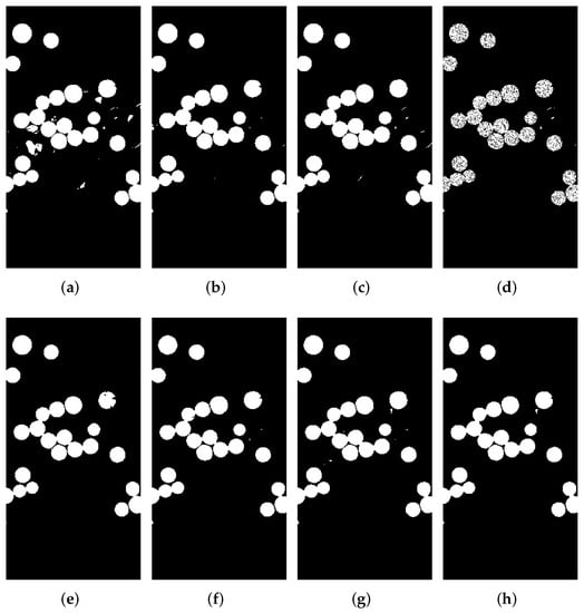
Figure 7.
The change map on Umatilla dataset. (a) CVA. (b) IRMAD. (c) ISFA. (d) SVM. (e) GETNET. (f) 2DCNN. (g) 3DCNN. (h) ours.

Table 2.
Quantitative evaluation of CD results by different methods for Umatilla dataset.
4.3.3. Experiments on the Yancheng Dataset
The changes in this dataset are mainly related to farmland. The results are shown in Figure 8 and listed in Table 3. The Yancheng dataset is a relatively simple, traditional method that can also achieve a good performance, especially the performance of ISFA and deep-learning methods that are very similar. Additionally, their OAs are all over . The performance of SVM is the worst and there is too much noise in the changed area. In addition, these four deep-learning methods have all performed very well, but GETNET and 2DCNN still have obvious noise in the unchanged regions, and 3DCNN performs poorly in the changed regions. Only our method eliminates the background noise and also ensures the accuracy of the changed region with multiple iterations.
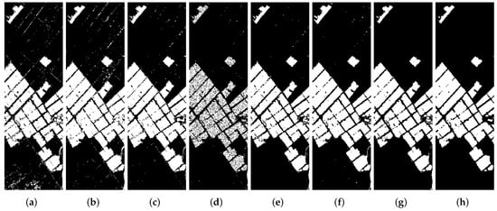
Figure 8.
The change map on Yancheng dataset. (a) CVA. (b) IRMAD. (c) ISFA. (d) SVM. (e) GETNET. (f) 2DCNN. (g) 3DCNN. (h) ours.

Table 3.
Quantitative evaluation of CD results by different methods for Yancheng dataset.
4.3.4. Experiments on the River Dataset
The River dataset is more complex than the other datasets and contains a variety of changes, mainly the disappearance of substances in rivers. Figure 9 shows the maps obtained by eight methods and the quantitative comparison is shown in Table 4. It is obvious from the numerical indicators that the results of CVA are extremely unbalanced, and the number of false-positive samples is approximately 6 times that of the false-negative samples. In addition, ISFA, which performs relatively well in the other datasets, has the worst accuracy here. There is no significant difference among the results of the three networks. The OA can grow to more than , which once again proves that the deep neural network has a strong learning ability and that sample selection can effectively suppress noisy labels. Through multiple iterations and sample selection, the proposed method eliminates the huge deviation of the initial pseudo-labels and obtains the best performance.
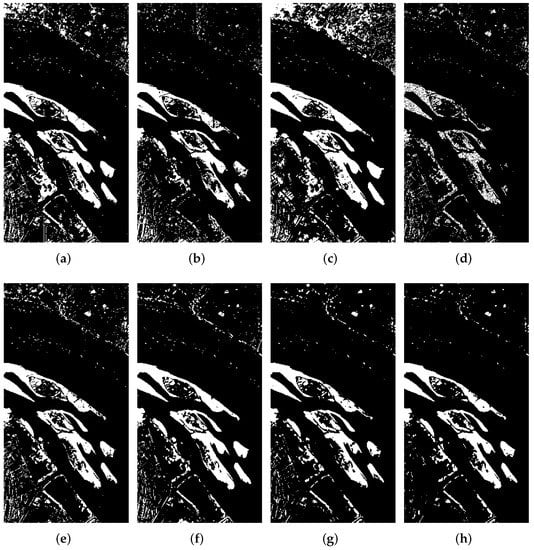
Figure 9.
The change map on River dataset. (a) CVA. (b) IRMAD. (c) ISFA. (d) SVM. (e) GETNET. (f) 2DCNN. (g) 3DCNN. (h) ours.

Table 4.
Quantitative evaluation of CD results by different methods for River dataset.
5. Discussion
5.1. Ablation Study
To argue the effectiveness of the mutual teaching paradigm, on the above four datasets we make the two networks perform mutual teaching and separate training under the same conditions. Figure 10 shows the OA of the results in 10 consecutive iterations. Classifiers A and B refer to each other’s predicted values, while A′ and B′ only use their own results. The two sets of experiments have the same initialization. In the mutual teaching framework, high-precision classifiers are often dragged down by low-precision classifiers, undergoing raising and lowering changes. However, overall, the performances of the two models basically show an upward trend. Although this process has some fluctuations, it does not affect the overall performance. The self-training performance is relatively poor, and the Umatilla and Yancheng datasets are almost not improved. The improvement of the Bastrop and River datasets is mainly due to sample selection and label correction, but it is also inferior to the mutual teaching models.
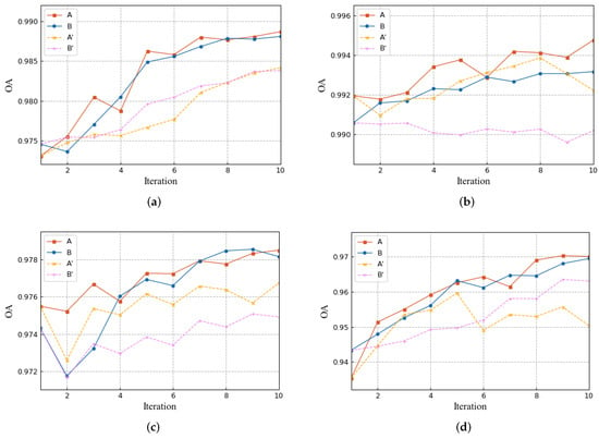
Figure 10.
The iterative performance of the mutual teaching framework, where A and B use mutual teaching and A′ and B′ are self-training. (a) Bastrop dataset. (b) Umatilla dataset. (c) Yancheng dataset. (d) River dataset.
As shown in Figure 11, we compare the alternating training with only one sample selection method. If a dataset itself is relatively simple, the difference between these results is not large. To show the difference in performance, we only use the most complicated River dataset. Figure 11 shows the overall accuracy of the final results and the variance between two models under three settings in each iteration on the River dataset. Although the model accuracy increases faster when only the group confidence-based sample selection method is used, the accuracy no longer increases and remains stable from the sixth iteration. The overall accuracy is further improved by alternating training and significantly exceeds other settings, which proves that the participation of complex samples in training is beneficial to improving the model performance and preserving the details of the change map.
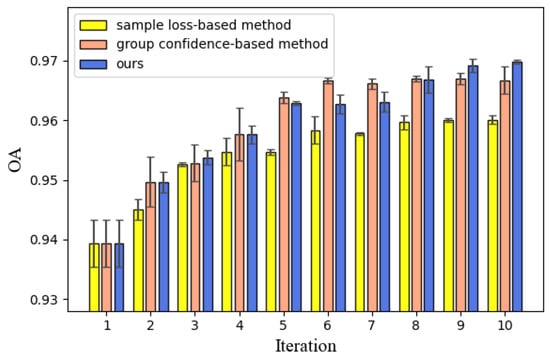
Figure 11.
The result accuracy and the variance of two models under three settings on River dataset.
5.2. Compatibility of the Proposed Framework with Other Models
Figure 12 displays the change detection results of three networks during initialization and after 10 iterations in our framework. GETNET and 3DCNN have considerably more false-positive samples during initialization, which is mainly misled by the pseudo-labels generated by CVA. However, after multiple corrections, these noises have been improved to a certain extent, especially for the 3DCNN (as shown in the red box). The main error of the 2DCNN result is that some changed regions were not detected, and it had also been recovered after iteration. In other words, both false-positive and false-negative noise labels have the opportunity to be corrected under the proposed framework. The results demonstrate that the mutual teaching framework can also benefit other deep-learning methods based on pseudo-labels.
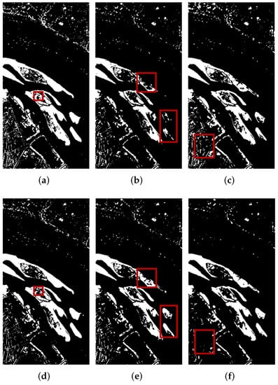
Figure 12.
Results of different networks in the first and last iterations on River dataset. (a) GETNET in the first iteration. (b) 2DCNN in the first iteration. (c) 3DCNN in the first iteration. (d) GETNET in the last iteration. (e) 2DCNN in the last iteration. (f) 3DCNN in the last iteration.
5.3. Hyperparametric Analysis
5.3.1. Analysis of the Pseudo-Label Update Rate
In the process of pseudo-label correction, the momentum parameter (in Equation (2)) selection is worth discussing. When , pseudo-labels in each iteration are determined only by new predicted values; when , our method depends entirely on the initial pseudo-label without any updates. We measure the results of different parameters on four datasets, as shown in Figure 13. Experimental results show that the update of pseudo-labels can bring a better performance. If the false labels are not corrected, they will inevitably limit the final result. With the increase in , the overall accuracy shows a downward trend. A value of 0.2∼0.5 is a suitable range for all datasets. Therefore, we choose for our experiments.
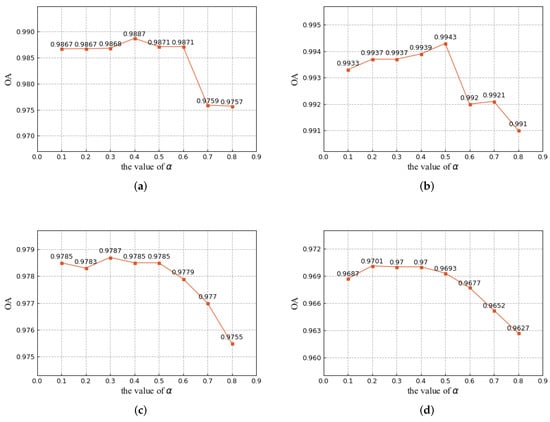
Figure 13.
Analysis of the momentum parameter . (a) Bastrop dataset. (b) Umatilla dataset. (c) Yancheng dataset. (d) River dataset.
5.3.2. Analysis of the Number of Groups
Sample selection by clustering methods can ensure the diversity of training samples. However, too detailed a classification makes it difficult to remove noise for datasets with simple ground objects types (the sample loss-based method is more effective here). For complicated datasets, especially HSI that are sensitive to ground changes, classified sampling is crucial to class balance and model generalization. The results for different numbers of groups are shown in Figure 14. Since the Bastrop dataset has only one change type, and the spectral information of MSI is much less than that of HSI, the value of n needs to be small. Based on the experiment, we choose on the Bastrop dataset. For the other three HSI datasets, we choose . Moreover, other clustering methods that automatically determine the number of groups can be considered to avoid parameter selection.
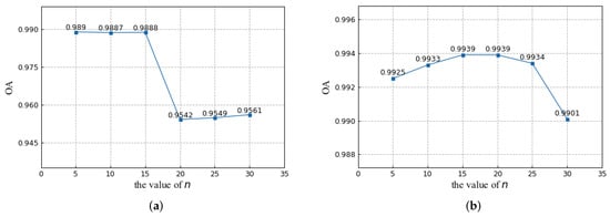
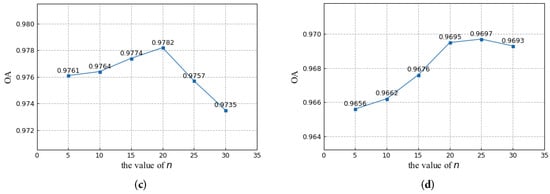
Figure 14.
Analysis of the number of groups n. (a) Bastrop dataset. (b) Umatilla dataset. (c) Yancheng dataset. (d) River dataset.
5.4. Computing Time
The computing device is equipped with Intel i7-9700K CPU (3.6 GHz) and NVIDIA GeForce RTX2080Ti GPU. The program is written in Python via the code library of PyTorch. Here, we list the computing time for each dataset in Table 5. With the multiple models and numerous iterations for optimization, the proposed method suffers from high computational complexity. Theoretically, the optimization process of the two models is independent. Therefore, the method can be accelerated by parallel computing to reduce the computing time by , which is the same as the self-training time of a single model.

Table 5.
Time cost (seconds) of each dataset.
6. Conclusions
In this article, a general mutual teaching framework with momentum correction is proposed for the HSI-CD task by dual-3DCNN. It aims to perform robust training for deep-learning methods using pseudo-labels generated by traditional approaches. Adopting the idea of collaborative training, the proposed framework encourages the two models to teach each other to mitigate self-confidence bias and boosts label correction in the iterative process to further improve performance. Then, focusing on the complexity of HSI change types, a new sample selection method based on group confidence is designed to extract better quality and diverse training data. Furthermore, the 3DCNN can effectively extract spatiotemporal spectral features of bitemporal HSIs, and thus, it is developed as the basic classifier of the above framework. Our approach uses pseudo-labels obtained by unsupervised algorithms, which means it can also be compatible with other networks that require labeled data.
We implemented our approach and performed experiments on a multispectral dataset, as well as on three public hyperspectral datasets. The visual and quantitative results show that our method can effectively improve the robustness and generalization of the deep neural network for the HSI-CD task.
Author Contributions
Conceptualization, J.S. and L.H.; methodology, L.X.; software, J.S.; validation, J.S., L.X. and J.L.; formal analysis, L.X. and J.L.; writing—original draft preparation, J.S.; writing—review and editing, L.X. and J.L.; visualization, J.S., L.H. and Z.W.; supervision, L.X., J.L. and Z.W.; project administration, L.X.; funding acquisition, L.X. All authors have read and agreed to the published version of the manuscript.
Funding
This research was funded by the National Natural Science Foundation of China under Grant 61571230, 61871226, and 61906093, in part by the Jiangsu Provincial Social Developing Project under Grant BE2018727, in part by the Jiangsu Provincial Nature Science Foundations of China under Grant BK20190451, in part by the Fundamental Research Funds for the Central Universities under Grant 30918011104 and 30920021134; and in part by the National Major Research Plan of China under Grant 2016YFF0103604.
Institutional Review Board Statement
Not applicable.
Informed Consent Statement
Not applicable.
Data Availability Statement
Not applicable.
Conflicts of Interest
The authors declare no conflict of interest.
References
- Scafutto, R.D.M.; de Souza Filho, C.R.; de Oliveira, W.J. Hyperspectral remote sensing detection of petroleum hydrocarbons in mixtures with mineral substrates: Implications for onshore exploration and monitoring. ISPRS J. Photogramm. Remote Sens. 2017, 128, 146–157. [Google Scholar] [CrossRef]
- Carrino, T.A.; Crósta, A.P.; Toledo, C.L.B.; Silva, A.M. Hyperspectral remote sensing applied to mineral exploration in southern Peru: A multiple data integration approach in the Chapi Chiara gold prospect. Int. J. Appl. Earth Obs. Geoinf. 2018, 64, 287–300. [Google Scholar] [CrossRef]
- Zhang, X.; Sun, Y.; Shang, K.; Zhang, L.; Wang, S. Crop classification based on feature band set construction and object-oriented approach using hyperspectral images. IEEE J. Sel. Top. Appl. Earth Obs. Remote Sens. 2016, 9, 4117–4128. [Google Scholar] [CrossRef]
- Vali, A.; Comai, S.; Matteucci, M. Deep learning for land use and land cover classification based on hyperspectral and multispectral earth observation data: A review. Remote Sens. 2020, 12, 2495. [Google Scholar] [CrossRef]
- Shimoni, M.; Haelterman, R.; Perneel, C. Hypersectral imaging for military and security applications: Combining myriad processing and sensing techniques. IEEE Geosci. Remote Sens. Mag. 2019, 7, 101–117. [Google Scholar] [CrossRef]
- Singh, A. Review article digital change detection techniques using remotely-sensed data. Int. J. Remote Sens. 1989, 10, 989–1003. [Google Scholar] [CrossRef] [Green Version]
- Bovolo, F.; Bruzzone, L. A theoretical framework for unsupervised change detection based on change vector analysis in the polar domain. IEEE Trans. Geosci. Remote Sens. 2006, 45, 218–236. [Google Scholar] [CrossRef] [Green Version]
- Celik, T. Unsupervised change detection in satellite images using principal component analysis and k-means clustering. IEEE Geosci. Remote Sens. Lett. 2009, 6, 772–776. [Google Scholar] [CrossRef]
- Nielsen, A.A.; Conradsen, K.; Simpson, J.J. Multivariate alteration detection (MAD) and MAF postprocessing in multispectral, bitemporal image data: New approaches to change detection studies. Remote Sens. Environ. 1998, 64, 1–19. [Google Scholar] [CrossRef] [Green Version]
- Nielsen, A.A. The regularized iteratively reweighted MAD method for change detection in multi-and hyperspectral data. IEEE Trans. Image Process. 2007, 16, 463–478. [Google Scholar] [CrossRef] [Green Version]
- Coppin, P.; Jonckheere, I.; Nackaerts, K.; Muys, B.; Lambin, E. Review ArticleDigital change detection methods in ecosystem monitoring: A review. Int. J. Remote Sens. 2004, 25, 1565–1596. [Google Scholar] [CrossRef]
- Wu, C.; Du, B.; Zhang, L. Slow feature analysis for change detection in multispectral imagery. IEEE Trans. Geosci. Remote Sens. 2013, 52, 2858–2874. [Google Scholar] [CrossRef]
- Ahlqvist, O. Extending post-classification change detection using semantic similarity metrics to overcome class heterogeneity: A study of 1992 and 2001 US National Land Cover Database changes. Remote Sens. Environ. 2008, 112, 1226–1241. [Google Scholar] [CrossRef]
- Wan, L.; Xiang, Y.; You, H. A post-classification comparison method for SAR and optical images change detection. IEEE Geosci. Remote Sens. Lett. 2019, 16, 1026–1030. [Google Scholar] [CrossRef]
- Liu, T.; Yang, L.; Lunga, D. Change detection using deep learning approach with object-based image analysis. Remote Sens. Environ. 2021, 256, 112308. [Google Scholar] [CrossRef]
- Mou, L.; Bruzzone, L.; Zhu, X.X. Learning spectral-spatial-temporal features via a recurrent convolutional neural network for change detection in multispectral imagery. IEEE Trans. Geosci. Remote Sens. 2018, 57, 924–935. [Google Scholar] [CrossRef] [Green Version]
- Wang, Q.; Yuan, Z.; Du, Q.; Li, X. GETNET: A general end-to-end 2-D CNN framework for hyperspectral image change detection. IEEE Trans. Geosci. Remote Sens. 2018, 57, 3–13. [Google Scholar] [CrossRef] [Green Version]
- Chen, Y.; Jiang, H.; Li, C.; Jia, X.; Ghamisi, P. Deep feature extraction and classification of hyperspectral images based on convolutional neural networks. IEEE Trans. Geosci. Remote Sens. 2016, 54, 6232–6251. [Google Scholar] [CrossRef] [Green Version]
- Du, B.; Ru, L.; Wu, C.; Zhang, L. Unsupervised deep slow feature analysis for change detection in multi-temporal remote sensing images. IEEE Trans. Geosci. Remote Sens. 2019, 57, 9976–9992. [Google Scholar] [CrossRef] [Green Version]
- Li, X.; Yuan, Z.; Wang, Q. Unsupervised deep noise modeling for hyperspectral image change detection. Remote Sens. 2019, 11, 258. [Google Scholar] [CrossRef] [Green Version]
- Li, Q.; Gong, H.; Dai, H.; Li, C.; He, Z.; Wang, W.; Feng, Y.; Han, F.; Tuniyazi, A.; Li, H.; et al. Unsupervised Hyperspectral Image Change Detection via Deep Learning Self-generated Credible Labels. IEEE J. Sel. Top. Appl. Earth Obs. Remote Sens. 2021, 14, 9012–9024. [Google Scholar] [CrossRef]
- Zhang, C.; Bengio, S.; Hardt, M.; Recht, B.; Vinyals, O. Understanding deep learning (still) requires rethinking generalization. Commun. ACM 2021, 64, 107–115. [Google Scholar] [CrossRef]
- Yu, X.; Han, B.; Yao, J.; Niu, G.; Tsang, I.; Sugiyama, M. How does disagreement help generalization against label corruption? In Proceedings of the International Conference on Machine Learning, Long Beach, CA, USA, 10–15 June 2019; pp. 7164–7173. [Google Scholar]
- Yao, Q.; Yang, H.; Han, B.; Niu, G.; Kwok, J.T.Y. Searching to exploit memorization effect in learning with noisy labels. In Proceedings of the International Conference on Machine Learning, Virtual Event, 13–18 July 2020; pp. 10789–10798. [Google Scholar]
- Shang, R.; Yuan, Y.; Jiao, L.; Meng, Y.; Ghalamzan, A.M. A self-paced learning algorithm for change detection in synthetic aperture radar images. Signal Proc. 2018, 142, 375–387. [Google Scholar] [CrossRef] [Green Version]
- Gong, M.; Duan, Y.; Li, H. Group self-paced learning with a time-varying regularizer for unsupervised change detection. IEEE Trans. Geosci. Remote Sens. 2019, 58, 2481–2493. [Google Scholar] [CrossRef]
- Han, B.; Yao, Q.; Yu, X.; Niu, G.; Xu, M.; Hu, W.; Tsang, I.; Sugiyama, M. Co-teaching: Robust Training of Deep Neural Networks with Extremely Noisy Labels. In Proceedings of the International Conference on Neural Information Processing Systems, Stockholm, Sweden, 10–15 July 2018; pp. 8536–8546. [Google Scholar]
- Li, P.; Xu, Y.; Wei, Y.; Yang, Y. Self-correction for human parsing. arXiv 2020, arXiv:1910.09777. [Google Scholar] [CrossRef]
- Zheng, G.; Awadallah, A.H.; Dumais, S. Meta label correction for noisy label learning. In Proceedings of the AAAI Conference on Artificial Intelligence, Virtual Event, 2–9 February 2021. [Google Scholar]
- Liu, J.; Gong, M.; Qin, K.; Zhang, P. A deep convolutional coupling network for change detection based on heterogeneous optical and radar images. IEEE Trans. Neural Netw. Learn. Syst. 2016, 29, 545–559. [Google Scholar] [CrossRef] [PubMed]
- Zhang, P.; Gong, M.; Zhang, H.; Liu, J.; Ban, Y. Unsupervised difference representation learning for detecting multiple types of changes in multitemporal remote sensing images. IEEE Trans. Geosci. Remote Sens. 2018, 57, 2277–2289. [Google Scholar] [CrossRef]
- Liu, J.; Zhang, W.; Liu, F.; Xiao, L. A Probabilistic Model Based on Bipartite Convolutional Neural Network for Unsupervised Change Detection. IEEE Trans. Geosci. Remote Sens. 2021, 60, 4701514. [Google Scholar] [CrossRef]
- Gong, M.; Zhao, J.; Liu, J.; Miao, Q.; Jiao, L. Change detection in synthetic aperture radar images based on deep neural networks. IEEE Trans. Neural Netw. Learn. Syst. 2015, 27, 125–138. [Google Scholar] [CrossRef]
- Li, Y.; Peng, C.; Chen, Y.; Jiao, L.; Zhou, L.; Shang, R. A deep learning method for change detection in synthetic aperture radar images. IEEE Trans. Geosci. Remote Sens. 2019, 57, 5751–5763. [Google Scholar] [CrossRef]
- Goldberger, J.; Ben-Reuven, E. Training deep neural-networks using a noise adaptation layer. In Proceedings of the International Conference of Learning Representations (ICLR), San Juan, Puerto Rico, 2–4 May 2016. [Google Scholar]
- Ghosh, A.; Kumar, H.; Sastry, P. Robust loss functions under label noise for deep neural networks. In Proceedings of the AAAI Conference on Artificial Intelligence, San Francisco, CA, USA, 4–9 February 2017; Volume 31. [Google Scholar]
- Lee, K.H.; He, X.; Zhang, L.; Yang, L. Cleannet: Transfer learning for scalable image classifier training with label noise. In Proceedings of the IEEE Conference on Computer Vision and Pattern Recognition, Salt Lake City, UT, USA, 18–22 June 2018; pp. 5447–5456. [Google Scholar]
- Jiang, L.; Zhou, Z.; Leung, T.; Li, L.J.; Li, F.-F. Mentornet: Learning data-driven curriculum for very deep neural networks on corrupted labels. In Proceedings of the International Conference on Machine Learning, PMLR, Stockholm, Sweden, 10–15 July 2018; pp. 2304–2313. [Google Scholar]
- Blum, A.; Mitchell, T. Combining labeled and unlabeled data with co-training. In Proceedings of the Eleventh Annual Conference on Computational Learning Theory, Madison, WI, USA, 24–26 July 1998; pp. 92–100. [Google Scholar]
- Zhang, Y.; Xiang, T.; Hospedales, T.M.; Lu, H. Deep mutual learning. In Proceedings of the IEEE Conference on Computer Vision and Pattern Recognition, Salt Lake City, UT, USA, 18–22 June 2018; pp. 4320–4328. [Google Scholar]
- Ge, Y.; Chen, D.; Li, H. Mutual mean-teaching: Pseudo label refinery for unsupervised domain adaptation on person re-identification. In Proceedings of the International Conference on Learning Representations, Addis Ababa, Ethiopia, 26–30 April 2020. [Google Scholar]
- Yang, F.; Li, K.; Zhong, Z.; Luo, Z.; Sun, X.; Cheng, H.; Guo, X.; Huang, F.; Ji, R.; Li, S. Asymmetric co-teaching for unsupervised cross-domain person re-identification. In Proceedings of the AAAI Conference on Artificial Intelligence, New York, NY, USA, 7–12 February 2020; Volume 34, pp. 12597–12604. [Google Scholar]
- Liu, J.; Li, R.; Sun, C. Co-Correcting: Noise-tolerant Medical Image Classification via mutual Label Correction. IEEE Trans. Med. Imag. 2021, 40, 3580–3592. [Google Scholar] [CrossRef] [PubMed]
- Tai, X.; Li, M.; Xiang, M.; Ren, P. A Mutual Guide Framework for Training Hyperspectral Image Classifiers with Small Data. IEEE Trans. Geosci. Remote Sens. 2021, 60, 5510417. [Google Scholar] [CrossRef]
- Lin, T.Y.; Goyal, P.; Girshick, R.; He, K.; Dollár, P. Focal loss for dense object detection. In Proceedings of the IEEE International Conference on Computer Vision, Venice, Italy, 22–29 October 2017; pp. 2980–2988. [Google Scholar]
- Volpi, M.; Camps-Valls, G.; Tuia, D. Spectral alignment of multi-temporal cross-sensor images with automated kernel canonical correlation analysis. ISPRS J. Photogramm. Remote Sens. 2015, 107, 50–63. [Google Scholar] [CrossRef]
Publisher’s Note: MDPI stays neutral with regard to jurisdictional claims in published maps and institutional affiliations. |
© 2022 by the authors. Licensee MDPI, Basel, Switzerland. This article is an open access article distributed under the terms and conditions of the Creative Commons Attribution (CC BY) license (https://creativecommons.org/licenses/by/4.0/).