An Investigation of a Multidimensional CNN Combined with an Attention Mechanism Model to Resolve Small-Sample Problems in Hyperspectral Image Classification

Abstract

The convolutional neural network (CNN) method has been widely used in the classification of hyperspectral images (HSIs). However, the efficiency and accuracy of the HSI classification are inevitably degraded when small samples are available. This study proposes a multidimensional CNN model named MDAN, which is constructed with an attention mechanism, to achieve an ideal classification performance of CNN within the framework of few-shot learning. In this model, a three-dimensional (3D) convolutional layer is carried out for obtaining spatial–spectral features from the 3D volumetric data of HSI. Subsequently, the two-dimensional (2D) and one-dimensional (1D) convolutional layers further learn spatial and spectral features efficiently at an abstract level. Based on the most widely used convolutional block attention module (CBAM), this study investigates a convolutional block self-attention module (CBSM) to improve accuracy by changing the connection ways of attention blocks. The CBSM model is used with the 2D convolutional layer for better performance of HSI classification purposes. The MDAN model is applied for classification applications using HSI, and its performance is evaluated by comparing the results with the support vector machine (SVM), 2D CNN, 3D CNN, 3D–2D–1D CNN, and CBAM. The findings of this study indicate that classification results from the MADN model show overall classification accuracies of 97.34%, 96.43%, and 92.23% for Salinas, WHU-Hi-HanChuan, and Pavia University datasets, respectively, when only 1% HSI data were used for training. The training and testing times of the MDAN model are close to those of the 3D–2D–1D CNN, which has the highest efficiency among all comparative CNN models. The attention model CBSM is introduced into MDAN, which achieves an overall accuracy of about 1% higher than that of the CBAM model. The performance of the two proposed methods is superior to the other models in terms of both efficiency and accuracy. The results show that the combination of multidimensional CNNs and attention mechanisms has the best ability for small-sample problems in HSI classification.

1. Introduction

Hyperspectral images (HSIs) are three-dimensional (3D) volumetric data with a spectrum of continuous and narrow bands, which can reflect the characteristics of ground objects in detail [1]. In recent years, many mini-sized and low-cost HSI sensors have appeared, which makes it easy to obtain HSI data with rich spatial–spectral information, such as AisaKESTREL10, AisaKESTREL16, and FireflEYE [2,3]. In this context, HSI is widely used in the fields of resource detection, environmental analysis, disaster monitoring, etc. [4,5,6]. The classification of HSI is a basic analysis task that has become very popular [7]. However, due to the influence of the small number of samples (small samples), the high-dimensional characteristics, the similarity between the spectra, and the mixed pixels, efficient and accurate classification of HSI data has been a challenging task for many years [8,9,10]. To solve these problems, some deep learning network models have been applied in HSI processing [11], especially the convolutional neural network (CNN).

Recently, CNN has attracted extensive attention due to its efficacy in many visual applications, for instance, classification, object detection, and semantic segmentation [12,13,14]. Three types of CNNs—namely, one-dimensional (1D), two-dimensional (2D), and three-dimensional CNNs—are successfully applied in HSI classification tasks. The 1D and 2D CNNs can obtain more abstract level spectral or spatial features of HSI [15]. The 3D CNN can learn the structural spatial–spectral feature representation using a 3D core, which can comprehensively characterize ground objects [16]. Recently, 3D CNNs have attracted extensive attention in HSI classification. Li et al. presented a novel approach that uses a 3D CNN to view HSI cube data altogether [17]. Mayra et al. used a 3D CNN to show the great potential of using HSI to map tree species [18]. Although these two 3D CNN models offer a simple and effective method for HSI classification, their accuracy and efficiency can be still further improved.

As can be seen from the literature, the results of using a single CNN of the three CNNs have a few shortcomings in achieving high accuracy [19]. The main reason is that HSI data are volumetric data and have information representation in both spatial and spectral dimensions. The 1D CNN and 2D CNN alone are not able to extract discriminating feature maps from both spatial and spectral dimensions. Similarly, a deep 3D CNN is more computationally complex, and it is difficult to classify a large volume of HSI data with its use. In addition, the performance of using a 3D CNN alone cannot satisfy the analysis of classes with similar textures over many spectral bands [19]. To address these issues, hybrid CNNs for HSI classification are developed. Swalpa et al. proposed a hybrid spectral CNN model (HybridSN), which assembles the 3D and 2D convolutional layers for reducing the complexity of the 3D CNN model [19]. Zhang et al. used a 3D–1D CNN model and showed improved accuracy in the classification of vegetation species [16]. Since the performance of these two models is still limited for classification applications in the condition of ground scenes with many different land cover types, a hybrid 3D–2D–1D CNN has been proposed by Liu et al. [20]. Notably, it does not perform well in terms of accuracy when the sample data are small. In this study, a new model that makes full use of multidimensional CNNs is proposed and uses some refinement mechanisms to overcome these shortcomings of the previous methods.

Moreover, for the problem of small samples, an attention mechanism was applied to an HSI analysis task [21,22]. The attention mechanism is a resource allocation scheme that can improve the performance of a model with a little computational complexity [23], such as the squeeze-and-excitation networks (SENets) [24], the selective kernel networks (SKNets) [25], the convolutional block attention module (CBAM) [26], and the bottleneck attention module (BAM) [27]. Compared with SENet, SKNet, and BAM, CBAM is a lightweight model, and it can extract attention features in spatial–spectral dimensions for adaptive feature refinement. Considering HSI is a 3D feature map, CBAM is selected to enhance the expression ability of the HSI classification model. Additionally, to make it applicable to the characteristics of HSI and obtain a higher accuracy of the classification using HSI, a convolutional block self-attention module named CBSM is also proposed based on the CBAM.

For the application of the CBSM model, this study proposes a multidimensional CNN with an attention mechanism model named MDAN. The MDAN model contains three types of CNNs components and the CBSM model for higher efficiency and accuracy of classification purposes.

The main contributions of this study are as follows:

• An improved graph convolutional network MDAN is proposed for HSI classification with small samples;
• A multidimensional CNN and a classical attention mechanism CBAM are used to create deeper feature maps from small samples;
• Based on CBAM, an attention module CBSM is designed to improve HSI classification accuracy. The CBSM has increased connections, which is more suitable for the classification of HSI data. Comparative experiments are carried out on three open datasets, and the experimental results indicate that the MDAN model and the CBSM model are superior to other state-of-the-art HSI classification models.

The rest of the paper is organized as follows: Section 2 introduces the proposed MDAN and CBSM. Section 3 presents the parameter settings and the results of the proposed approaches on the three different HSI datasets. The discussion of the results is described in Section 4. Finally, the conclusions are shown in Section 5.

2. MDAN and CBSM Models

2.1. MDAN Model

The structure of the MDAN model is demonstrated in Figure 1. It can be seen that MDAN uses the characteristics of all three types of CNNs and an attention mechanism CBSM to extract different features from small samples. The spatial spectrum’s representation features are extracted by two 3D convolutional layers from the input data. The spatial features are obtained at the 2D convolutional layer from the spatial-spectrum features. The spatial features are modified by the attention module CBSM, which is set between the 2D convolutional and 1D convolutional layers, to improve the classification accuracy. The 1D convolutional layer is performed to further extract spectral features; then, the classification is carried out based on spectral enhancement information.

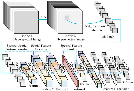
Figure 1. Architecture of the MDAN model; notably, the attention module CBSM is used to obtain the modified Feature 4.

In the MDAN model, the original input HSI data cube is denoted by $\mathrm{I}\in R^{H\times W\times B}$, where $H$, $W$ and $B$ are the height, width, and the number of spectral bands, respectively. The band number of one pixel in I is equal to $B$, and the pixel contains rich feature information for a label vector $y\in R^{1\times 1\times M}$, where $M$ denotes the classes of ground objects. However, HSI data contain narrow and continuous bands, high intraclass variability, and interclass similarity; thus, it is a considerable challenge for the classification of HSI tasks [28]. In this case, the principal component analysis (PCA) is commonly used to decrease the spectral feature dimensions of the original input data cube $\mathrm{I}$, and the output data are denoted by $\mathrm{X}\in R^{H\times W\times D}$, where D is the number of the spectral bands after the PCA is used [29,30,31].

2.2. CBSM Model

CBSM is an attention model for improving the accuracy of the HSI classification for the problems of small samples, as portrayed in Figure 2. Let the intermediate HSI feature map be denoted by $F\in R^{H\times W\times C}$, where, C is the number of the spectral bands of the input map. CBSM can be regarded as a dynamic-weight adjustment process to identify salient regions in complex scenes through the 1D channel attention map denoted by $M_C\in R^{1\times 1\times C}$, and the 2D spatial attention map denoted by $M_S\in R^{H\times W\times 1}$. During the processes of CBSM, the input data are refined sequentially by $M_C$ and $M_S$. As a result, the overall process of CBSM can be written as

$$F^{\prime }=M_c\left(F\right)\times F+F=(M_c\left(F\right)+1)\times F,$$

(1)

$$F^{″}=M_s(F^{\prime })\times F^{\prime }+F^{\prime }=(M_s(F^{\prime })+1)\times F^{\prime },$$

(2)

where $\times$ represents the multiplication by the element, and $+$ denotes the elementwise addition. In the computational process of the multiplication, the refined map $M_C$ and $M_S$ are broadcasted accordingly to form a 3D attention map—the channel attention map $M_C$ is broadcasted following the spatial dimension, and the spatial attention map $M_S$ is broadcasted following the spectral dimension. Then, all the 3D attention maps are multiplied with the input map $F$ or $F^{\prime }$ in an elementwise manner. In the computational process of the addition, the process between two maps denotes that two elements in the same 3D spatial position are added together, and the process between the $+1$ and a map represents each element of the map plus 1. $F^{\prime }$ indicate the intermediate feature map refined by $M_C$. $F^{″}$ is the final refined feature map through the CBSM model, which is illustrated in Figure 2.

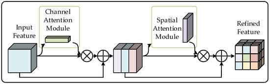
Figure 2. Structure of CBSM.

$M_C$ is generated by pooling the weight of each channel feature. First, for determining the relationship representation between channels efficiently, feature F is squeezed along the spatial dimension. In this step, two parallel branches, i.e., global-average-pooling (GAP) and global-max-pooling (GMP) operations are used for the feature extraction of each image. The two parallel branches output two parallel spatial context features, i.e., $F_{avg}^c$ and $F_{max}^c$. Then, the two features are delivered to a shared network, which consists of a multilayer perceptron (MLP) and one hidden layer, generating two intermediate features denoted as $W_1\in R^{C\times C/r}$. In the shared network, the value of hidden activation is set to $R^{1\times 1\times \left(C/r\right)}$ for computational efficiency, where $r$ is the reduction ratio. Finally, the output feature vectors $W_1$ are merged by element to produce the channel attention map $M_C\in R^{1\times 1\times C}$, which is computed as

$$\begin{gathered} M_c\left(F\right)=\sigma \left(MLP\left(GAP\left(F\right)\right)+MLP\left(GMP\left(F\right)\right)\right)=\sigma (W_1\left(W_O\left(F_{avg}^c\right)\right)+ \\ {W}_1\left(W_O\left(F_{max}^c\right)\right)), \end{gathered}$$

(3)

where $\sigma$ represents the sigmoid function, which maps variables into the range of $0–1$. In the process of the MLP, the rectified linear unit (ReLU) activation function is followed by $W_O\in R^{C/r\times C}$. It is noted that $W_O$ and $W_1$, are shared for both inputs.

$M_S$ is generated by pooling the weight of each spatial feature. First, the input map is computed in the two processes of GAP and GMP along the channel dimension to generate two 2D maps, i.e., $F_{avg}^s\in R^{H\times W\times 1}$ and $F_{max}^s\in R^{H\times W\times 1}$. These maps are then concatenated and convolved through a standard convolution layer, producing the 2D map, i.e., $M_S\in R^{H\times W\times 1}$, which encodes locations to emphasize or suppress. Consequently, the spatial attention of CBSM is computed as

$$M_s\left(F\right)=\sigma \left(f^{7\times 7}\left(\left[GAP\left(F\right);GMP\left(F\right)\right]\right)\right)=\sigma \left(f^{7\times 7}\left(\left[F_{avg}^s;F_{max}^s\right]\right)\right),$$

(4)

where $f^{7\times 7}$ denotes a 2D CNN filtering with the size of $7\times 7$.

The above two attention maps are complementary in CBSM, and they can capture rich contextual dependencies to enhance representation power in both the spectral and spatial dimensions of the input map.

3. Experiments and Results

3.1. Datasets

Three test datasets of Salinas (SA), WHU-Hi-HanChuan (WHU), and Pavia University (PU) datasets were selected for validating the MDAN and CBSM models. The WHU dataset contains high-quality data collected from a city in central China, which belongs to an agricultural area in a combined urban and rural region, and it was used as a benchmark dataset for the test results. Different from this dataset, SA and PU datasets were broadly used in the verification of HSI classification algorithms [32,33].

3.1.1. The SA Dataset

The SA dataset was collected by an AVIRIS sensor in 1992 in the Salinas Valley area of the United States. This dataset has a spatial resolution of 3.7 m, a spectral resolution of $9.7–12 \mathrm{nm}$, and a spectral range of $0.40–2.50 \mathsf{\mu }\mathrm{m}$. In this dataset, the image size is 512 × 217 pixels, and the number of labeled classes is 16. It composes 224 bands, including 20 bands with atmospheric moisture absorption and a low signal-to-noise ratio should be deleted. In this study, 204 bands were retained for the experiments. Figure 3a shows the ground truth of the land cover of the SA dataset. Table 1 shows the real mark classes of the dataset, the s of samples in the training, and the testing set.

Figure 3. Ground truth of the three datasets: (a) SA; (b) WHU; (c) PU. It should be noted that the category number of the datasets denoted by the color bar on the right represents the same category number as Table 1, Table 2 and Table 3.

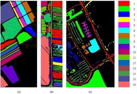
Table 1. The SA dataset.

Category No.	Class	Samples	Training Samples	Testing Samples
1	Broccoli-green weeds_1	2009	20	1989
2	Broccoli-green weeds_2	3726	37	3689
3	Fallow	1976	20	1956
4	Fallow rough plow	1394	14	1380
5	Fallow smooth	2678	27	2651
6	Stubble	3959	40	3919
7	Celery	3579	36	3543
8	Grapes untrained	11,271	113	11,158
9	Soil vineyard develop	6203	62	6141
10	Corn senesced green weeds	3278	33	3245
11	Lettuce romaine 4wk	1068	11	1057
12	Lettuce romaine 5wk	1927	19	1908
13	Lettuce romaine 6wk	916	9	907
14	Lettuce romaine 7wk	1070	11	1059
15	Vineyard untrained	7268	73	7195
16	Vineyard vertical trellis	1807	18	1789

3.1.2. The WHU Dataset

The WHU dataset was acquired by an 8 mm focal length Headwall Nano-Hyperspec imaging sensor in 2016 in HanChuan, Hubei Province, China. The image of the WHU dataset contains $1217\times 303$ pixels with a spatial resolution of 0.109 m and 274 bands, with a wavelength range of $0.40–1.00 \mathsf{\mu }\mathrm{m}$. Since the dataset was acquired during the afternoon, when the solar elevation angle was low, many shadow-covered areas are shown in the image. Figure 3b shows the ground truth of the land cover of the WHU dataset. Table 2 shows the real mark classes of the dataset, the number of samples in the training, and the testing set.

Table 2. The WHU dataset.

Category No.	Class	Samples	Training Samples	Testing Samples
1	Strawberry	44,735	358	44,288
2	Cowpea	22,753	182	22,525
3	Soybean	10,287	82	10,184
4	Sorghum	5353	43	5299
5	Water spinach	1200	10	1188
6	Watermelon	4533	36	4488
7	Greens	5903	47	5844
8	Trees	17,978	144	17,798
9	Grass	9469	76	9374
10	Red roof	10,516	84	10,411
11	Gray roof	16,911	135	16,742
12	Plastic	3679	29	3642
13	Bare soil	9116	73	9025
14	Road	18,560	148	18,374
15	Bright object	1136	9	1125
16	Water	75,401	603	74,647

3.1.3. The PU Dataset

The PU dataset was obtained by the ROSIS-03 sensor, which captures the urban area of Pavia. The size of the dataset is 610 × 340 pixels, and the spatial resolution is about 1.3 m. The dataset consists of 115 bands and 9 main ground objects, with a wavelength range of 0.43–0.86 μm. After removing 12 bands with high noise, the remaining 103 bands were selected for the experiments. Figure 3c shows the ground truth of the land cover of the PU dataset. Table 3 shows the real mark classes of the dataset, the number of samples in the training, and the testing set.

Table 3. The PU dataset.

Category No.	Class	Samples	Training Samples	Testing Samples
1	Strawberry	44,735	66	6565
2	Cowpea	22,753	186	18,463
3	Soybean	10,287	21	2078
4	Sorghum	5353	31	3033
5	Water spinach	1200	13	1332
6	Watermelon	4533	50	4979
7	Greens	5903	13	1317
8	Bright object	1136	37	3645
9	Water	75,401	9	938

3.2. Experimental Parameter Settings

The MDAN model contains two 3D convolutional layers, one 2D convolutional layer, one CBSM module, one 1D convolutional layer, one flatten layer, and two fully connected layers. In the experiments, the patch sizes of the three datasets were set to $25\times 25\times 15$, where 15 denotes the value of D, i.e., the number of the remaining spectral parameters in the remote sensing image reduced by the PCA. The patch size was determined according to studies by [19,34]; thus, one patch could roughly cover one single class. Empirically, the epochs of the training data were set to 20 for all three datasets, as the convergence of the MDAN model was achieved within the 20 epochs. The optimal learning rate was set to 0.001, also based on the above literature. For each class, only 1% of the pixels were randomly selected for model training, and the remaining 99% of the pixels were used for performance evaluation. Thus, the minimum number of training samples was close to 10 in all three datasets. Finally, two fully connected layers were used to connect all neurons with the Adam optimizer. Across the board, the MDAN model was randomly initialized and trained by the back-propagation algorithm with no batch normalization and data augmentation. The class probability vector of each pixel was generated through the MDAN model and then was compared with the real label on the ground for the performance evaluation of MDAN. The experiment was carried out under the environment of the Windows 10 operating system and NVIDIA Geforce RTX 2080ti graphics card. More details on class information are provided in Table 4, where Run CBSM Here denotes that the CBSM process was carried out at this position in the MDAN Process.

Table 4. Layer summary of the MDAN model based on the PU dataset.

CBSM Process			MDAN Process
Layer (Type)	Output Shape	Parameter	Layer (Type)	Output Shape	Parameter
Global_Average_Pooling2D_1	Globa (32)	0	Input Layer	(25, 25, 15, 0)	0
Global_Max_Pooling2D_1	Almax (32)	0	Conv3D_1	(23, 23, 9, 8)	512
Reshape_1	(1, 1, 32)	0	Conv3D_2	(21, 21, 5, 16)	5776
Reshape_2	(1, 1, 32)	0	Reshape_1	(21, 21, 80)	0
Dense_1	(1, 1, 4)	132	Conv2D_1	(19, 19, 32)	23,072
Dense_2	(1, 1, 32)	160	Run CBSM Here
Add_1	(1, 1, 32)	0
Activation_1	(1, 1, 32)	0	Reshape_2	(19, 608)	0
Multiply_1	(19, 19, 32)	0	Conv1D_1	(17, 64)	116,800
Tf_Operators_Add_1	Lambd (19, 19, 32)	0	Flatten_1	(1088)	0
Lambda_1	(19, 19, 1)	0	Dense_1	(256)	278,784
Lambda_2	(19, 19, 1)	0	Dropout_1	(256)	0
Concatenate_1	(19, 19, 2)	0	Dense_2	(128)	32,896
Conv2D_1	(19, 19, 1)	98	Dropout_2	(128)	0
Multiply_2	(19, 19, 32)	0	Dense_3	(9)	1161
Tf_Operators_Add_2	Oplam (19, 19, 32)	0	Total params: 459,391
Add_2	(19, 19, 32)	0

In the two 3D convolutional layers, the dimensions of the 3D convolution kernels are $8\times 3\times 3\times 7\times 1$ and $16\times 3\times 3\times 5\times 8$; the latter means 3D kernels have the number of 16, and the dimension of $3\times 3\times 5$ for all 8 3D input feature maps, $3\times 3$, and 5 means the spatial and the spectral dimension of the 3D kernels, respectively. In the 2D convolutional layers, the size of the kernel is $32\times 3\times 3\times 80$, where 32 is the number of the 2D kernels with the size of $3\times 3$, and 80 represents the size of the 2D input data. The CBSM model was used to improve classification accuracy with the two attention maps, in which the channel attention was implemented by GAP and GMP operation across the spatial dimension; the spatial attention module has the characteristics of GAP and GMP in the channel dimension with a convolution kernel size of $7\times 7$. Finally, in the 1D convolution layer, the kernel size is $64\times 3\times 608$, where 64 is the spectral dimension of the 1D kernels, and 608 indicates the size of the 1D input data. For the practical efficiency of the model, the 3D, 2D, and 1D convolution layers were used before the flatten layer. The 3D layer can extract the spatial–spectral information in one convolution process. The 2D layer can strongly discriminate the spatial information within different bands. The 1D layer can strengthen and compress the spectral information for efficient classification. It can be observed from Table 4 that in the PU dataset, the parameters take up to 278784 at the dense_1 layer of the MDAN Process. The number of the nodes in the Dense_3 layer at the end of the MDAN Process is nine, which depends on the number of the real label classes. In this case, the total number of the trainable weight parameters in the MDAN model is 459,391.

3.3. Classification Results

In this section, the overall accuracy (OA), average accuracy (AA), Kappa coefficient (KAPPA), training time, and testing time evaluation measures are used to assess the performance of the two proposed approaches. The OA is obtained by dividing correctly classified samples by all the test samples in a dataset; the AA denotes the average accuracies of all classes, which is as important as OA. When the sample is unbalanced, the accuracy will be biased towards multiple classes. In this case, the KAPPA needs to be obtained for a consistency test. The closer the KAPPA is to 1, the higher the consistency is. Finally, the efficiency of the MDAN model is reflected by the training and testing time.

The results of the two models are compared with the most broadly used methods, including the support vector machine (SVM) [35], 2D CNN [36], 3D CNN [37], and CBAM [26]. For a further evaluation of the classification performance of the two models, the 3D–2D–1D CNN [20] and the intermediate model of 3D–2D–CBAM–1D CNN are also compared with the MDAN model. Table 5 shows the results of the three datasets.

Table 5. Classification accuracies and efficiencies of the proposed two models and selected methods using the WHU, SA, and PU datasets, respectively, and the best performances are highlighted in bold.

		SVM	2D CNN	3D CNN	3D–2D–1D CNN	3D–2D–CBAM–1D CNN (New)	MDAN (3D–2D–CBSM–1D CNN, New)
SA	OA (%)	82.48	97.25	77.40	94.46	96.16	97.34
	AA (%)	83.92	97.79	77.96	94.69	96.82	97.22
	KAPPA (×100)	80.47	96.94	74.61	93.83	95.72	97.04
	Running time (s)	0.02	190.13	42.75	23.74	31.03	26.29
	Testing time (s)	1.87	187.84	43.53	34.10	43.13	38.19
WHU	OA (%)	76.34	94.57	85.98	94.10	95.59	96.43
	AA (%)	53.23	86.81	78.06	84.35	88.69	90.72
	KAPPA (×100)	72.16	93.62	83.66	93.08	94.83	95.81
	Running time (s)	0.20	857.86	199.17	108.17	121.12	122.26
	Testing time (s)	36.06	1128.30	207.97	160.94	176.01	183.09
PU	OA (%)	63.83	89.26	60.59	85.03	90.64	92.23
	AA (%)	37.24	80.79	43.50	68.98	83.25	83.21
	KAPPA (×100)	43.74	85.44	47.54	80.16	87.62	89.65
	Running time (s)	0.55	172.10	34.88	18.98	20.74	21.37
	Testing time (s)	7.42	152.44	34.19	26.94	29.80	29.98

The test results of the three datasets classification are shown in Table 6, Table 7 and Table 8, respectively, and the best performances are highlighted in bold. Obviously, the MDAN model achieves a good classification accuracy in almost all classes. The accuracy of the model of SVM and 3D CNN is slightly lower.

Table 6. Classification accuracies of the SA dataset. This table shows the best performances in bold.

Classes	SVM	2D CNN	3D CNN	3D–2D–1D CNN	3D–2D–CBAM–1D CNN (New)	MDAN (3D–2D–CBSM–1D CNN, New)
Brocoli-green weeds_1	98.66	100.00	99.85	100.00	97.99	100.00
Brocoli-green weeds_2	98.42	100.00	100.00	99.70	100.00	100.00
Fallow	74.19	100.00	8.84	100.00	100.00	100.00
Fallow rough plow	72.24	100.00	97.54	100.00	100.00	89.28
Fallow smooth	93.43	98.49	79.63	75.67	95.51	98.87
Stubble	99.01	100.00	100.00	100.00	99.80	99.03
Celery	98.88	100.00	100.00	99.92	99.86	100.00
Grapes untrained	67.81	97.88	95.42	91.54	98.18	99.18
Soil vineyard develop	98.31	100.00	98.14	100.00	100.00	100.00
Corn senesced green weeds	87.34	98.24	97.81	99.63	94.42	98.37
Lettuce romaine 4wk	90.64	97.82	78.52	89.78	98.39	87.51
Lettuce romaine 5wk	79.76	99.95	1.68	78.20	99.48	94.92
Lettuce romaine 6wk	80.79	86.00	95.81	97.35	86.11	100.00
Lettuce romaine 7wk	49.72	100.00	95.94	93.67	97.83	99.91
Vinyard untrained	62.37	86.28	6.61	89.76	81.57	88.44
Vinyard vertical trellis	91.20	100.00	91.62	99.78	100.00	100.00

Table 7. Classification accuracies of the WHU dataset. This table shows the best performances in bold.

Classes	SVM	2D CNN	3D CNN	3D–2D–1D CNN	3D–2D–CBAM–1D CNN (New)	MDAN (3D–2D–CBSM–1D CNN, New)
Strawberry	88.83	99.82	71.31	99.01	99.79	99.34
Cowpea	69.93	92.28	92.41	90.08	88.25	97.24
Soybean	48.32	96.43	85.67	94.49	98.87	96.28
sorghum	80.74	99.34	98.53	98.64	99.94	98.75
Water spinach	12.33	99.49	92.26	98.06	95.54	97.73
Watermelon	11.43	69.52	66.29	35.41	65.98	83.04
Greens	65.70	90.69	93.67	88.72	92.88	93.94
Trees	54.48	90.42	63.63	95.04	95.56	94.48
Grass	37.98	89.28	94.69	86.13	86.87	96.50
Red roof	76.99	94.54	84.55	98.73	98.38	95.70
Gray roof	83.41	96.45	94.76	95.22	98.13	97.14
Plastic	16.09	60.90	38.74	52.14	88.96	73.20
Bare soil	31.59	76.38	51.90	80.58	81.12	82.19
Road	75.50	91.87	95.50	95.87	95.02	93.62
Bright object	0.18	41.78	25.16	41.69	33.87	52.44
Water	98.20	99.82	99.84	99.82	99.82	99.88

Table 8. Classification accuracies of the PU dataset. This table shows the best performances in bold.

Classes	SVM	2D CNN	3D CNN	3D–2D–1D CNN	3D–2D–CBAM–1D CNN (New)	MDAN (3D–2D–CBSM–1D CNN, New)
Asphalt	65.47	93.24	0.08	93.02	80.11	90.39
Meadows	99.37	99.98	99.81	94.80	98.71	99.70
Gravel	19.25	77.91	8.66	13.67	83.06	83.30
Trees	10.67	77.65	80.12	85.06	88.46	78.47
Painted metal sheets	6.69	96.10	99.92	95.05	99.17	96.40
Bare soil	26.07	73.11	0.00	99.90	98.79	99.96
Bitumen	23.68	82.99	0.00	41.31	89.37	76.99
Self-blocking bricks	43.56	75.78	85.73	67.74	75.03	80.25
Shadows	40.44	50.37	17.18	30.31	36.50	43.44

The test results are illustrated in Figure 4, Figure 5 and Figure 6, and the category number is the same as that in Table 1, Table 2 and Table 3. It is found that, in the selected models, there are some ground objects with low accuracy in the marked area of the yellow circle. The MDAN model can solve this problem and provides the highest accuracy for most ground objects. However, the results of MDAN have some misclassified in the marked area of the red circle. The points in the red circles in each figure are too small to avoid the reduction in the overall accuracy of the MDAN model.

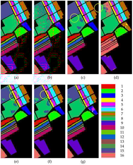
Figure 4. Ground truth and classification results of the SA dataset: (a) ground truth; (b) SVM; (c) 2D CNN; (d) 3D CNN; (e) 3D–2D–1D CNN; (f) 3D–2D–CBAM–1D CNN; (g) MDAN (3D–2D–CBSM–1D CNN). This figure shows the classes with lower classification accuracy in the yellow circle and the red circle.

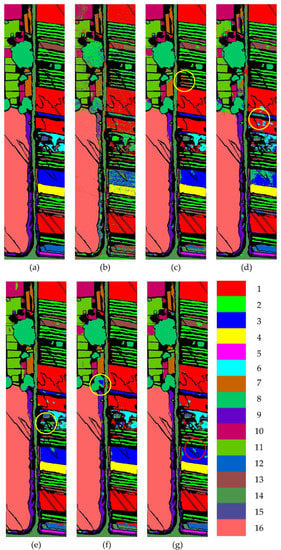
Figure 5. Ground truth and classification results of the WHU dataset: (a) ground truth; (b) SVM; (c) 2D CNN; (d) 3D CNN; (e) 3D–2D–1D CNN; (f) 3D–2D–CBAM–1D CNN; (g) MDAN (3D–2D–CBSM–1D CNN). This figure shows the classes with lower classification accuracy in the yellow circle and the red circle.

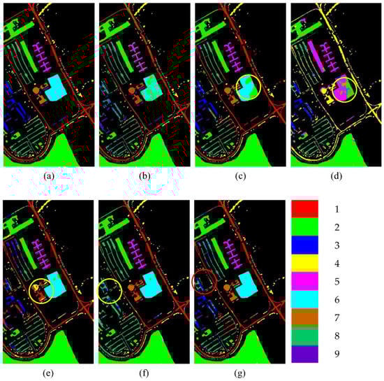
Figure 6. Ground truth and classification results of the PU dataset: (a) ground truth; (b) SVM; (c) 2D CNN; (d) 3D CNN; (e) 3D–2D–1D CNN; (f) 3D–2D–CBAM–1D CNN; (g) MDAN (3D–2D–CBSM–1D CNN). This figure shows the classes with lower classification accuracy in the yellow circle and the red circle.

Figure 7 portrays the confusion matrices of the proposed MDAN model using all the three selected datasets. It can be seen that the MDAN model achieves correct classification in almost all classes. The training curves for 100 epochs of the three datasets are shown in Figure 8 for the MDAN model. It indicates that in roughly 20 epochs, the MDAN model roughly reaches perfect convergence.

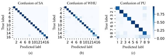
Figure 7. The confusion matrices of MDAN in the three selected datasets: (a) the confusion of the SA dataset; (b) the confusion of the WHU dataset; (c) the confusion of the PU dataset.

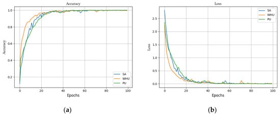
Figure 8. Accuracies and loss convergence versus epochs of the proposed MDAN model using on the WHU, SA, and PU datasets: (a) accuracies; (b) loss.

According to studies in the literature, the algorithms for HSI classification are sensitive to unbalanced datasets in the predictor classes [23,38]. A model developed based on unbalanced datasets tends to result in false predictions in small samples, but the overall accuracy of the predictions is not necessarily low. Therefore, supplementary experiments are further carried out using balanced training samples, i.e., all ground objects have the same number of samples. Among all three datasets, the PU dataset is a more representative dataset, with medium spatial resolutions, lower accuracy, and a diverse set of ground scenes; thus, the PU dataset was only used for the following experiments. In this study, the training epoch was set to 100, and the range of the training samples was set to $10–70$. Table 9 shows the supplementary experiment results.

Table 9. Classification results of MDAN using a balanced training sample of the PU dataset.

Classes	10	20	30	40	50	60	70
Asphalt	71.88	83.54	94.38	93.78	97.77	96.15	98.47
Meadows	97.83	97.28	99.02	99.64	98.75	99.74	99.74
Gravel	14.84	73.21	66.97	79.10	87.92	88.95	89.56
Trees	55.66	87.35	84.01	88.58	85.46	90.31	86.32
Painted metal sheets	90.16	95.74	98.65	99.78	95.27	95.56	96.30
Bare soil	50.82	99.58	93.10	99.36	99.84	100.00	99.98
Bitumen	11.23	82.25	90.77	61.71	96.73	97.18	96.80
Self-blocking bricks	82.04	57.57	79.58	91.67	85.12	90.35	90.02
Shadows	4.66	57.48	60.26	72.31	84.95	68.98	83.17
OA (%)	74.83	88.71	92.16	94.43	95.59	96.31	96.71
AA (%)	53.23	81.55	85.19	87.33	92.42	91.91	93.37
KAPPA (×100)	65.48	85.04	89.53	92.60	94.16	95.10	95.62
Running time (s)	23.34	44.22	64.70	85.92	104.97	125.97	146.32
Testing time (s)	30.05	30.08	29.98	30.25	29.98	29.77	29.91
Asphalt	71.88	83.54	94.38	93.78	97.77	96.15	98.47

As shown in Table 9, 20 samples can roughly meet the required accuracy in the low training time of the HSI classification; hence, it is promising for the application and popularization of the MDAN model. Then, with the expansion of the number of training samples, the accuracy increases slowly. The highest classification accuracy is achieved in the case of 50 samples; thus, more training samples (i.e., 60 or 70) are not necessarily needed for the use of the MDAN model in the task of HSI classification.

4. Discussion

The results of the proposed models and the selected models are shown in Figure 4, Figure 5, Figure 6, Figure 7, Figure 8, Table 5, Table 6, Table 7, Table 8 and Table 9. It can be seen that the MDAN model achieves the best performance among all of the selected models in terms of both accuracy and efficiency and achieves the overall accuracies of 97.34%, 92.23%, and 96.42%, respectively, in the test results of the SA, PU, and WHU datasets. In addition, compared with the two basic algorithms of 2D CNN and 3D CNN, the efficiency of MDAN is significantly improved. Additionally, compared with the 3D–2D–1D CNN, which is the most efficient model among all of the selected CNN models, MDAN takes slightly longer in terms of training and testing times. Different from the selected CNN models, the SVM model achieves the lowest accuracy but the highest efficiency among all of the selected models; thus, it is suitable for the situation of HSI classification that does not require high accuracy but needs high efficiency.

The classification results of the 2D CNN indicate lower efficiency but higher accuracy than those of the 3D CNN in the case of small samples. However, if the samples are sufficiently large, the 3D CNN is better capable of extracting discriminating features than the 2D CNN; then, the accuracy of the 3D CNN can meet the most requirements [37]. This is because the 3D CNN can obtain higher-level features than the 2D CNN and can further reduce the number of training samples. In general, a CNN model needs massive volumes of data for a good performance; thus, the classification accuracy of the 3D CNN is lower than that of the 2D CNN with small samples when the valid information of the HSI features is removed. Moreover, the 2D CNN retains more parameters, which tend to consume a large amount of time in the stage of using a classifier. As a result, the efficiency of the 2D CNN is the lowest efficiency among all selected models.

In the case of small samples, the hybrid 3D–2D–1D CNN is more efficient and accurate than the 3D CNN. However, the accuracy of this hybrid model is not as good as that of the 2D CNN, and it is reduced in the results of the SA and PU datasets, while it remains the same in the results of the WHU dataset. Therefore, this method still can be improved regarding the accuracy of the classification using HSI.

The accuracy of the 3D–2D–CBAM–1D CNN is higher than that of the hybrid 3D–2D–1D CNN model. In addition, the 2D and the 1D convolutional layers are incorporated in the hybrid model for high efficiency; thus, the CBAM model is also used between the 2D and 1D convolutional layers to form the 3D–2D–CBAM–1D CNN for high accuracy. CBAM is a spatial-spectrum attention module, which significantly improves the performance of a vision task based on its rich representation power [26]. As shown in Table 3, this model achieves an accuracy improvement, as expected by using CBAM. However, due to the unique high-dimensional spectral characteristics of HSI, the best performance cannot be achieved by CBAM only, and the accuracy of the 3D–2D–CBAM–1D CNN is close to that of the 2D CNN.

According to the literature on attention models, different attention connections lead to different classification results [39,40,41]. Thus, the CBSM attention module with different attention structural connections from CBAM is proposed to suit the 3D characteristics of HSI data. CBSM can significantly improve CNN’s ability to classify HSI data, and the application of CBSM in MDAN, i.e., 3D–2D–CBSM–1D CNN further improves the accuracy from the CBAM used in 3D–2D–CBAM–1D CNN by 1%. Compared with the selected models of the SVM, 2D CNN,3D CNN, 3D–2D–1D CNN, and 3D–2D–CBAM–1D CNN, the MDAN model is the best performer on all three datasets. In addition, the MDAN model also performs well in balanced training samples and correctly classifies all classes, as shown in Table 4.

In summary, since the application of the attention mechanism, the MDAN model can make CNN more efficient and more accurate in HSI classification than other selected CNN models for small-sample problems. The attention module CBSM can further improve the accuracy of the HSI classification model and can be easily integrated into other CNN models to improve model performance.

5. Conclusions

In this study, to address the poor accuracy of HSI classification models on the small samples in the training data, an improved graph model MDAN was proposed from the perspective of multidimensional CNNs and attention mechanisms. The MDAN model can efficiently extract and refine features to obtain better performance in terms of both accuracy and efficiency. To make the model more suitable for HSI data structure, an attention module CBSM was also proposed in this study, which provided a better connection method than the most widely used CBAM model. The CBSM module was used in the MDAN model; thus, the spatial–spectral features were further refined, resulting in a model that significantly helps to improve the accuracy of the HSI classification under the condition of small samples. A series of comparative experiments were carried out using three open HSI datasets. The experiment results indicated that the combination of multidimensional CNN and attention mechanisms has a better performance on HSI data among all of the selected models using both balanced and unbalanced small samples. The connection method used in the CBSM model is more suitable for the extraction and classification of HSI data and further improved the accuracy.

However, the performance of CBSM is better than CBAM only in the connection method. Hence, future studies will be focused on finding a more targeted attention module for HSI data. Moreover, the accuracy improvement made by new models is still limited; thus, other strategies, such as supplementing the small samples using open high-dimensional spectral data, may be used in the future. In addition, future research will also focus on transfer learning and the samples randomly selected from anywhere when a large number of rich HSI data appear.

References

- Qing, Y.; Liu, W. Hyperspectral Image Classification Based on Multi-Scale Residual Network with Attention Mechanism. Remote Sens. 2021, 13, 335. [Google Scholar] [CrossRef]
- Lu, B.; Dao, P.D.; Liu, J.; He, Y.; Shang, J. Recent Advances of Hyperspectral Imaging Technology and Applications in Agriculture. Remote Sens. 2020, 12, 2659. [Google Scholar] [CrossRef]
- Zhong, Y.; Wang, X.; Xu, Y.; Wang, S.; Jia, T.; Hu, X.; Zhao, J.; Wei, L.; Zhang, L. Mini-UAV-Borne Hyperspectral Remote Sensing: From Observation and Processing to Applications. IEEE Geosci. Remote Sens. Mag. 2018, 6, 46–62. [Google Scholar] [CrossRef]
- Krupnik, D.; Khan, S. Close-Range, Ground-Based Hyperspectral Imaging for Mining Applications at Various Scales: Review and Case Studies. Earth-Sci. Rev. 2019, 198, 102952. [Google Scholar] [CrossRef]
- Jia, J.; Wang, Y.; Chen, J.; Guo, R.; Shu, R.; Wang, J. Status and Application of Advanced Airborne Hyperspectral Imaging Technology: A Review. Infrared Phys. Technol. 2020, 104, 103115. [Google Scholar] [CrossRef]
- Seydi, S.T.; Akhoondzadeh, M.; Amani, M.; Mahdavi, S. Wildfire Damage Assessment over Australia Using Sentinel-2 Imagery and MODIS Land Cover Product within the Google Earth Engine Cloud Platform. Remote Sens. 2021, 13, 220. [Google Scholar] [CrossRef]
- Cai, W.; Liu, B.; Wei, Z.; Li, M.; Kan, J. Triple-Attention Guided Residual Dense and BiLSTM Networks for Hyperspectral Image Classification. Multimed. Tools Appl. 2021, 80, 11291–11312. [Google Scholar] [CrossRef]
- Wang, W.; Liu, X.; Mou, X. Data Augmentation and Spectral Structure Features for Limited Samples Hyperspectral Classification. Remote Sens. 2021, 13, 547. [Google Scholar] [CrossRef]
- Paoletti, M.E.; Haut, J.M.; Plaza, J.; Plaza, A. A New Deep Convolutional Neural Network for Fast Hyperspectral Image Classification. ISPRS-J. Photogramm. Remote Sens. 2018, 145, 120–147. [Google Scholar] [CrossRef]
- Xu, X.; Li, J.; Wu, C.; Plaza, A. Regional Clustering-Based Spatial Preprocessing for Hyperspectral Unmixing. Remote Sens. Environ. 2018, 204, 333–346. [Google Scholar] [CrossRef]
- Jia, S.; Jiang, S.; Lin, Z.; Li, N.; Xu, M.; Yu, S. A Survey: Deep Learning for Hyperspectral Image Classification with Few Labeled Samples. Neurocomputing 2021, 448, 179–204. [Google Scholar] [CrossRef]
- Sultana, F.; Sufian, A.; Dutta, P. Evolution of Image Segmentation using Deep Convolutional Neural Network: A Survey. Knowl.-Based Syst. 2020, 201, 62. [Google Scholar] [CrossRef]
- Sun, Y.; Xue, B.; Zhang, M.; Yen, G.G. Evolving Deep Convolutional Neural Networks for Image Classification. IEEE Trans. Evol. Comput. 2020, 24, 394–407. [Google Scholar] [CrossRef] [Green Version]
- Wan, S.; Goudos, S. Faster R-CNN for Multi-Class Fruit Detection Using A Robotic Vision System. Comput. Netw. 2020, 168, 107036. [Google Scholar] [CrossRef]
- Lv, W.; Wang, X. Overview of Hyperspectral Image Classification. J. Sens. 2020, 2020, 4817234. [Google Scholar] [CrossRef]
- Zhang, B.; Zhao, L.; Zhang, X. Three-Dimensional Convolutional Neural Network Model for Tree Species Classification Using Airborne Hyperspectral Images. Remote Sens. Environ. 2020, 247, 111938. [Google Scholar] [CrossRef]
- Ying, L.; Haokui, Z.; Qiang, S. Spectral–Spatial Classification of Hyperspectral Imagery with 3D Convolutional Neural Network. Remote Sens. 2017, 9, 67. [Google Scholar] [CrossRef] [Green Version]
- Mayra, J.; Keski-Saari, S.; Kivinen, S.; Tanhuanpaa, T.; Hurskainen, P.; Kullberg, P.; Poikolainen, L.; Viinikka, A.; Tuominen, S.; Kumpula, T.; et al. Tree Species Classification From Airborne Hyperspectral and LiDAR Data Using 3D Convolutional Neural Networks. Remote Sens. Environ. 2021, 256, 112322. [Google Scholar] [CrossRef]
- Roy, S.K.; Krishna, G.; Dubey, S.R.; Chaudhuri, B.B. HybridSN: Exploring 3-D–2-D CNN Feature Hierarchy for Hyperspectral Image Classification. IEEE Geosci. Remote Sens. Lett. 2020, 17, 277–281. [Google Scholar] [CrossRef] [Green Version]
- Jinxiang, L.; Wei, B.; Yu, C.; Yaqin, S.; Huifu, Z.; Erjiang, F.; Kefei, Z. Multi-Dimensional CNN Fused Algorithm for Hyperspectral Remote Sensing Image Classification. ChJL 2021, 48, 1610003. [Google Scholar] [CrossRef]
- Xiong, Z.; Yuan, Y.; Wang, Q. AI-NET: Attention Inception Neural Networks for Hyperspectral Image Classification. In Proceedings of the 2018 IEEE International Geoscience and Remote Sensing Symposium (IGARSS), Valencia, Spain, 22–27 July 2018; pp. 2647–2650. [Google Scholar]
- Haut, J.M.; Paoletti, M.E.; Plaza, J.; Plaza, A.; Li, J. Visual Attention-Driven Hyperspectral Image Classification. ITGRS 2019, 57, 8065–8080. [Google Scholar] [CrossRef]
- Zhang, J.; Wei, F.; Feng, F.; Wang, C. Spatial–Spectral Feature Refinement for Hyperspectral Image Classification Based on Attention-Dense 3D-2D-CNN. Sensors 2020, 20, 5191. [Google Scholar] [CrossRef]
- Jie, H.; Li, S.; Albanie, S.; Gang, S.; Wu, E. Squeeze-and-Excitation Networks. ITPAM 2020, 42, 2011–2023. [Google Scholar] [CrossRef] [Green Version]
- Li, X.; Wang, W.; Hu, X.; Yang, J. Selective kernel networks. In Proceedings of the 2019 IEEE/CVF Conference on Computer Vision and Pattern Recognition (CVPR), Long Beach, CA, USA, 15–20 June 2019; pp. 510–519. [Google Scholar]
- Woo, S.; Park, J.; Lee, J.-Y.; Kweon, I.S. CBAM: Convolutional Block Attention Module. In Proceedings of the European Conference on Computer Vision (ECCV), Munich, Germany, 8–14 September 2018; pp. 3–9. [Google Scholar]
- Park, J.; Woo, S.; Lee, J.-Y.; Kweon, I.S. BAM: Bottleneck Attention Module. arXiv 2018, arXiv:1807.06514. [Google Scholar]
- Huang, H.; Shi, G.; He, H.; Duan, Y.; Luo, F. Dimensionality Reduction of Hyperspectral Imagery Based on Spatial–Spectral Manifold Learning. IEEE T. Cybern. 2019, 50, 2604–2616. [Google Scholar] [CrossRef] [PubMed] [Green Version]
- Haque, M.R.; Mishu, S.Z. Spectral-Spatial Feature Extraction Using PCA and Multi-Scale Deep Convolutional Neural Network for Hyperspectral Image Classification. In Proceedings of the 2019 22nd International Conference on Computer and Information Technology (ICCIT), Dhaka, Bangladesh, 18–20 December 2019; pp. 1–6. [Google Scholar]
- Yousefi, B.; Sojasi, S.; Castanedo, C.I.; Maldague, X.P.V.; Beaudoin, G.; Chamberland, M. Comparison Assessment of Low Rank Sparse-PCA Based-Clustering/Classification for Automatic Mineral Identification in Long Wave Infrared Hyperspectral Imagery. Infrared Phys. Technol. 2018, 93, 103–111. [Google Scholar] [CrossRef]
- Sellami, A.; Farah, M.; Riadh Farah, I.; Solaiman, B. Hyperspectral Imagery Classification Based on Semi-Supervised 3-D Deep Neural Network and Adaptive Band Selection. Expert Syst. Appl. 2019, 129, 246–259. [Google Scholar] [CrossRef]
- Imani, M.; Ghassemian, H. An Overview on Spectral and Spatial Information Fusion for Hyperspectral Image Classification: Current Trends and Challenges. Inf. Fusion 2020, 59, 59–83. [Google Scholar] [CrossRef]
- Zhong, Z.; Li, J.; Clausi, D.A.; Wong, A. Generative Adversarial Networks and Conditional Random Fields for Hyperspectral Image Classification. IEEE T. Cybern. 2020, 50, 3318–3329. [Google Scholar] [CrossRef] [PubMed] [Green Version]
- Yang, X.; Zhang, X.; Ye, Y.; Lau, R.Y.; Lu, S.; Li, X.; Huang, X. Synergistic 2D/3D Convolutional Neural Network for Hyperspectral Image Classification. Remote Sens. 2020, 12, 2033. [Google Scholar] [CrossRef]
- Melgani, F.; Bruzzone, L. Classification of Hyperspectral Remote Sensing Images with Support Vector Machines. ITGRS 2004, 42, 1778–1790. [Google Scholar] [CrossRef] [Green Version]
- Makantasis, K.; Karantzalos, K.; Doulamis, A.; Doulamis, N. Deep Supervised Learning for Hyperspectral Data Classification Through Convolutional Neural Networks. In Proceedings of the 2015 IEEE International Geoscience and Remote Sensing Symposium (IGARSS), Milan, Italy, 26–31 July 2015; pp. 4959–4962. [Google Scholar]
- Ben Hamida, A.; Benoît, A.; Lambert, P.; Ben Amar, C. 3-D Deep Learning Approach for Remote Sensing Image Classification. ITGRS 2018, 56, 4420–4434. [Google Scholar] [CrossRef] [Green Version]
- Li, X.; Li, Z.; Qiu, H.; Hou, G.; Fan, P. An Overview of Hyperspectral Image Feature Extraction, Classification Methods and The Methods Based on Small Samples. Appl. Spectrosc. Rev. 2021, 11, 1–34. [Google Scholar] [CrossRef]
- Guo, M.; Xu, T.; Liu, J.; Liu, Z.; Jiang, P.; Mu, T.; Zhang, S.; Martin, R.R.; Cheng, M.; Hu, S. Attention Mechanisms in Computer Vision: A Survey. arXiv 2021, arXiv:2111.07624. [Google Scholar]
- Yang, Z.; Zhu, L.; Wu, Y.; Yang, Y. Gated Channel Transformation for Visual Recognition. In Proceedings of the 2020 IEEE/CVF Conference on Computer Vision and Pattern Recognition (CVPR), Seattle, WA, USA, 13–19 June 2020; pp. 11791–11800. [Google Scholar]
- Ma, X.; Guo, J.; Tang, S.; Qiao, Z.; Chen, Q.; Yang, Q.; Fu, S. DCANet: Learning connected attentions for convolutional neural networks. arXiv 2020, arXiv:2007.05099. [Google Scholar]
Publisher’s Note: MDPI stays neutral with regard to jurisdictional claims in published maps and institutional affiliations. |
© 2022 by the authors. Licensee MDPI, Basel, Switzerland. This article is an open access article distributed under the terms and conditions of the Creative Commons Attribution (CC BY) license (https://creativecommons.org/licenses/by/4.0/).