Abstract
Multiple radio occultation (RO) missions are currently providing observations that are assimilated by the world’s leading numerical weather prediction centers. These RO missions use the same signals originating from the Global Navigation Satellite Systems (GNSS), but they have different satellite designs and sizes with different antennas and receivers. This results in different noise levels for different missions. Although the amplitude data are characterized by the Signal-to-Noise Ratio (SNR), the noise, to which they are normalized, is not the real Noise Floor (NF) of the RO observations. We study the statistical distributions of the SNR and NF for RO missions including COSMIC, COSMIC2, METOP-A, METOP-B, METOP-C, and Spire. We demonstrate that different missions have different NF values and different NF and SNR distributions, sometimes multimodal. We propose to use the most probable NF value as an SNR normalization constant in order to compare the SNR values from different RO missions.
1. Introduction
Presently there are several active radio occultation (RO) missions. First of all, COSMIC-2 should be mentioned [1,2,3,4]. COSMIC-2 followed COSMIC (Constellation Observing System for Meteorology, Ionosphere, and Climate). In the context of this study, its most important improvement is the higher Signal-to-Noise Ratio (SNR). The METOP (Meteorological Operational Satellite) mission, launched by EUMETSAT (European Organisation for the Exploitation of Meteorological Satellites), has been active for many years [5,6,7,8,9]. There are three METOP satellites: METOP-A, METOP-B, and METOP-C. COSMIC, COSMIC-2, and METOP data are freely available to the scientific community from the CDAAC (COSMIC Data Analysis and Archive Center) web-site https://cdaac-www.cosmic.ucar.edu, accessed on 5 December 2021.
Currently, there are also several commercial missions. Here, we can mention the Spire data [10,11,12,13,14], based on a large constellation of small nanosatellites with relatively low-gain antennas. The PlanetiQ mission uses a high-gain instrument [15], and the GeoOptics mission is based on CICERO (Community Initiative for Cellular Earth Remote Observation) [16]. Some of the commercial data are also provided for open access at the CDAAC Web-site.
Level 1b RO data, which are used for the profile inversion, include satellite orbit data, atmospheric excess phase, and amplitude, or SNR. SNR is nearly constant at large ray perigee heights (above 30 km), where it only indicates relatively small scintillations due to ionospheric propagation effects and measurement noise. As the ray immerses into the atmosphere, the regular refraction effects result in a decrease in the average amplitude, while multipath propagation contributes to stronger fluctuations. For measurements in the shadow zone, in most cases, the signal largely reduces to homogeneous incoherent noise, while the effects of deep propagation due to super-refraction [17] may create a coherent component. A general assumption is that the measurements in the shadow zone represent the additive white noise affecting the whole profile record [18]. The effect of this noise depends on the signal strength that is estimated from the SNR at high perigee altitude.
Higher SNR has advantages in the study of the troposphere and, in particular, the Planetary Boundary Layer (PBL) [15,17,19], where it is expected to contribute to improved retrieval quality. As pointed out by Sokolovskiy et al. [1] and Schreiner et al. [2], high SNR is most important for detecting deep signals in the tropical troposphere. Higher SNR is also expected to improve RO penetration depth. Nevertheless, lower SNR missions, such as Spire, have also been shown to provide good inversion results [10,11,12,13,14].
A quantitative characterization of the advantages of high SNR is, therefore, an important issue. In particular, the dependence of the penetration depth on the SNR was presented in [2]. SNR is provided in RO records in form of L1 and L2 channel amplitudes measured in [V/V]. By its definition, SNR is the signal amplitude divided by the noise level; however, there is no common definition of the noise level. For the Wave Optical (WO) inversion methods [20,21,22], the absolute calibration of the amplitude record has no importance. However, in order to compare different missions with different SNR, a common calibration is necessary. In this respect, we have to take a close look at such an important characteristic, as the background noise level [18], or the Noise Floor (NF). NF, being different for different missions, is a natural normalization constant in order to arrive at mission inter-comparable SNRs. Although different missions have a large difference in the nominal values of SNRs in [V/V], the normalized values may have a smaller difference due to different noise floors. This is important for making decisions on using low-SNR mission data. The use of inter-comparable SNRs may help to reduce of the number of mission-specific tuning parameters in RO processing and to arrive at a better definition of the profile bottom.
2. Data and Methods
RO observations include orbit data, phase excess , and amplitudes , where the lower index corresponds to the channel number. In this work, we only use the L1 channel data. We evaluate the climatological model of the phase excess . Our model employs MSISE-90 (Mass-Spectrometer-Incoherent-Scatter model Extended) [23], which describes the dry atmosphere. We complement MSISE-90 refractivity profile with constant relative humidity of 90% below 15 km. This model has been used for a long period of time, and it is proven to predict the Doppler frequency within 25 Hz [24]. From the model refractivity profile, we evaluate the bending angle profile , where is the bending angle, and is the ray impact parameter. This profile is exponentially extrapolated below the Earth’s surface. Given orbit data, this profile can be transformed into the parametric form . Because the model refractivity profile is a smooth function, this guarantees that both functions of time are single-valued. The extrapolation is used in order to cover the whole occultation event including the shadow zone. From the extended bending angle profile, we evaluate the model phase excess by inverting the standard geometric optical (GO) procedure of the evaluation of the bending angle from the excess phase [25]. The resulting excess phase model satisfies the requirements formulated by Sokolovskiy [24]: it is capable of describing the Doppler frequency with the accuracy of 10–15 Hz, which falls within the −25..25 Hz range corresponding to a 50 Hz sampling rate.
There are other climatological models tailored to GNSS RO data, such as BAROCLIM [26] or BAIAP [27]. These models were developed for use as the background in the statistical optimization, by averaging over a large ensemble of RO bending angles. They are good for large altitudes, but they are not so good in the lower troposphere, where their quality suffers from biases and limited penetration of RO events. Therefore, for the purpose of this study, the MSIS-based model is preferable.
The Wave Optical (WO) inversion methods [20,21,22] operate on the complex wave field:
where j is the channel number, , is the channel frequency, c is the light speed in a vacuum, and is the straight-line distance between the transmitting and occulting satellites. Generally, WO inversion methods are most effective for the L1 channel, which has a higher amplitude and a coarse-acquisition encoding with longer chips, which makes it more stable with respect to interference in multipath zones [28]. In this study, we only analyze the L1 channel, which allows omission of the channel index. Our model of the signal is as follows:
where is the true signal, and is a white noise, which has two components: is the inherent noise, and is the additional noise; . The basic assumption is that all the three components are uncorrelated. The root mean square (RMS) value of the inherent noise is used as the normalization constant for forming signal measured in [V/V]. Therefore, .
This model is based on the fact that RO measurements in the shadow zone, in most cases, represent a homogeneous uncorrelated signal [18]. This results in the natural definition of the signal strength measure , where is averaged for ray perigee altitudes, where the influence of the atmosphere upon the signal amplitude is negligible, and is averaged in the shadow zone. Because in practice, the signal level significantly exceeds the noise level (otherwise the measurements are not useful), we can write:
where the second-order term can be neglected, and the signal strength can be approximately expressed as . In the presence of deep propagation due to super-refraction [17], the signal in the shadow zone may have a coherent component superimposed on the noise. For specific events, this may result in an overestimate of the noise level; however, its value can be recovered by evaluating the statistical distributions from large ensembles of events.
Based on the above model of the signal, we evaluate two characteristics of the amplitude record: the mean SNR in the 60–80 km height range, , and the Noise Floor (NF) . The 60–80 km height range encompasses the ionospheric D-layer, and is optimal to estimate the signal strength that would be observed in the absence of an atmosphere. It is high enough for the attenuation due to the regular atmospheric refraction to be negligible. On the other hand, the influence of the ionosphere at these heights manifests itself in the small-scale fluctuations, which do not influence the average value. This height range does not reach the E-layer, where the amplitude perturbation can be stronger [29,30]. The average SNR in this height range as a measure of the signal strength was introduced in [31].
For each RO event, the mean SNR S is evaluated by averaging the L1 SNR for the samples with the model impact altitude within the interval of 60–80 km, where is local curvature radius of the reference ellipsoid cross-section by the occultation plane [32,33]. The NF F is evaluated by averaging the SNR for the samples with the model impact parameter below km. This choice is substantiated as follows. The impact altitude of a ray touching the Earth’s surface is estimated as , because at the Earth’s surface and km, km. The value of km was empirically chosen small enough to ensure that the observation is in the shadow zone. The estimate of the shadow zone is the only purpose for which the phase excess model is employed in this study.
By applying this procedure, we evaluate the set of pairs , where index i enumerates the RO events in the selected subset. From these data, we evaluate different 1-D and 2-D probability distributions. The “true” distributions are looked at as abstract concepts, because they can never be inferred from finite sets of realizations, they can only be estimated. There are two types of 1-D distributions: cumulative and differential ones, the latter being referred to as the Probability Distribution Function (PDF). Given a random value X, its cumulative distribution is defined as follows:
This function increases from to .
Numerically, it is estimated as follows. Given K random values , they are ranked in the ascending order : . Then, the set of pairs specifies the discrete representation of .
The differential distribution (PDF) is defined as the derivative of :
Numerically, it is estimated as follows. The whole set of is subdivided into intervals of length defined as the integer closest to : , where index l enumerates the intervals delimited by indexes . Then we define as a piecewise-constant function:
We start with the evaluation of the NF distributions. These distributions are evaluated for each mission, for each received GNSS constellation. For this study, we use COSMIC, COSMIC-2, METOP-A, -B, and -C, and Spire RO observations. COSMIC and METOP only receive GPS (denoted G). COSMIC-2 receives GPS and GLONASS (denoted R). For Spire, we use observations from GPS, GLONASS, Galileo (denoted E), and QZSS (denoted J). The most important characteristic of NF is its most probable value , because the corresponding PDFs have sharp peaks.
This results in the definition of two types of calibrated SNR: the dynamically normalized SNR and the normalized SNR , the latter definition referring to for the specific mission and GNSS. Because both S and F are measured in [V/V] and use the normalization to the inherent noise, evaluation of and corresponds to the normalization to the RMS of the overall noise instead of the inherent noise . We evaluate the 1-D distributions of and , as well as the 2-D joint distribution of . The latter is visualized in the form of scatter plots.
3. Results
For COSMIC, we selected 24 days of the year 2008 (1st and 15th day of each month), for a total of 61,905 events (GPS only). For COSMIC-2, we selected 24 days of the year 2020 (1st and 15th day of each month), for a total of 107,173 events: 69,657 GPS and 37,518 GLONASS events. For METOP-A, we selected the whole year 2020, for a total of 205,918 events (GPS only). For METOP-B, we selected the whole year 2020, for a total of 196,158 events (GPS only). For METOP-C, we selected the whole year 2020, for a total of 192,298 events (GPS only). For Spire, we selected 24 days (1st and 15th days of each month) of the year 2020 and, additionally, 8 days of 2021 (1st, 8th, 15th, and 22nd day of June and July), for a total of 282,824 events: 113,039 GPS, 77,821 GLONASS, 83,707 Galileo, and 8276 QZSS events. The Quality Control (QC) was reduced to a minimum: it was only required that it should be possible to determine S and F.
Figure 1, Figure 2, Figure 3, Figure 4, Figure 5, Figure 6, Figure 7, Figure 8, Figure 9 and Figure 10 show the distributions of , , and F for COSMIC, COSMIC-2, METOP-A,B,C, and Spire. Each figure contains four panels. The lower right panel shows the estimates of the cumulative and differential distributions (PDF) of NF. Each PDF has a sharp peak at the most probable value of NF, which is further used for the evaluation of the normalized SNRs plotted in the other three panels. The upper left panel shows the scatter plot visualizing the joint 2-D distribution of and , the former being normalized to the most probable value of NF, the latter being normalized to the dynamic value of NF evaluated for each event. The scatter plots of have the most complicated structure for GPS, as compared to the other GNSS constellations. The two remaining panels, upper right and lower left, show the cumulative and differential distributions of .
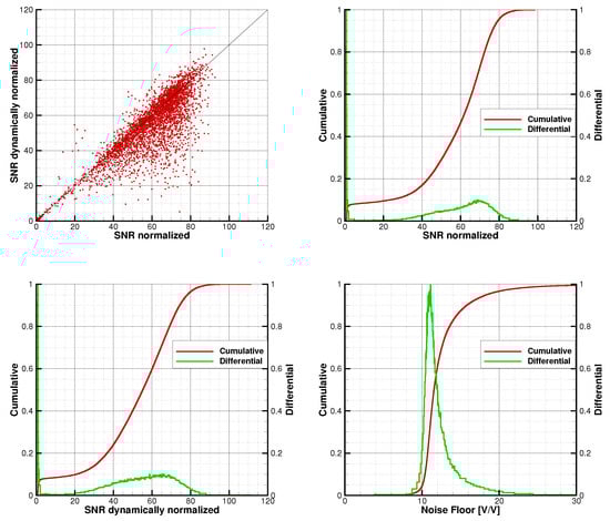
Figure 1.
SNR and noise floor statistics for COSMIC, GPS. Lower right: cumulative and differential distributions of the noise floor. The most probable value is used for the SNR normalization. Upper left: Scatter plot of dynamically normalized SNR (SNR over the dynamic estimate of the noise floor) vs. the SNR normalized to the most probable value of the noise floor. Upper right: the cumulative and differential distributions of normalized SNR. Lower left: the cumulative and differential distributions of dynamically normalized SNR.
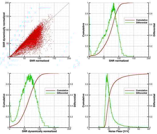
Figure 2.
SNR and noise floor statistics for COSMIC-2, GPS. Notation is the same as in Figure 1.
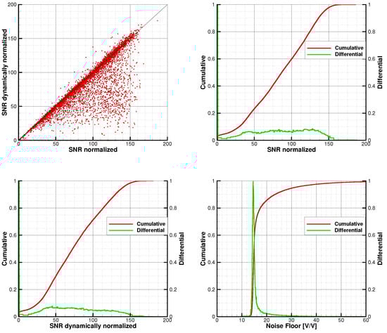
Figure 3.
SNR and noise floor statistics for COSMIC-2, GLONASS. Notation is the same as in Figure 1. GLONASS data indicate a stronger signal and a narrower NF distribution as compared to GPS.
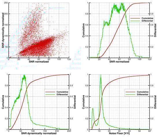
Figure 4.
SNR and noise floor statistics for METOP-A, GPS. Notation is the same as in Figure 1. The scatter plot of has a structure that is typical for GPS. Around 15% of events indicate two peaks of NF distribution, the lower peak value of 3.73 V/V being a technical artifact.
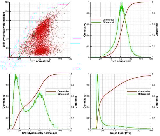
Figure 5.
SNR and noise floor statistics for METOP-B, GPS. Notation is the same as in Figure 1. The NF distribution has a bimodal structure, the second mode corresponding to large NF values. This corresponds to the secondary cloud for lower in the scatter plot of .
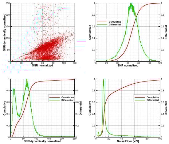
Figure 6.
SNR and noise floor statistics for METOP-C, GPS. Lower right: cumulative and differential distributions of the noise floor. Notation is the same as in Figure 1. The NF distribution indicates weaker features found for METOP-A (the false peak at lower NF) and METOP-C (the additional distribution mode for large NF).
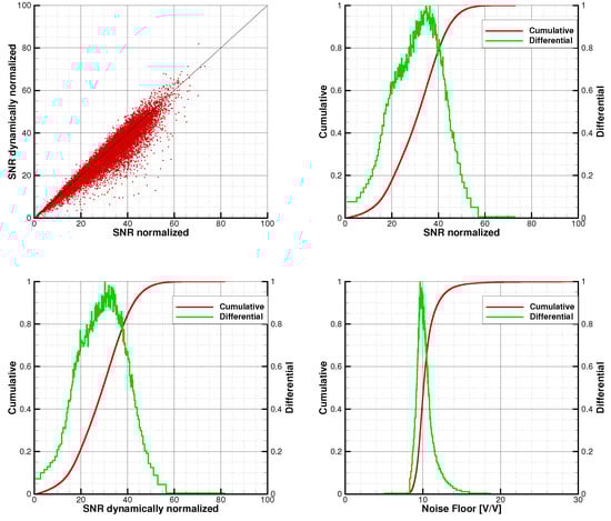
Figure 7.
SNR and noise floor statistics for Spire, GPS. Notation is the same as in Figure 1.
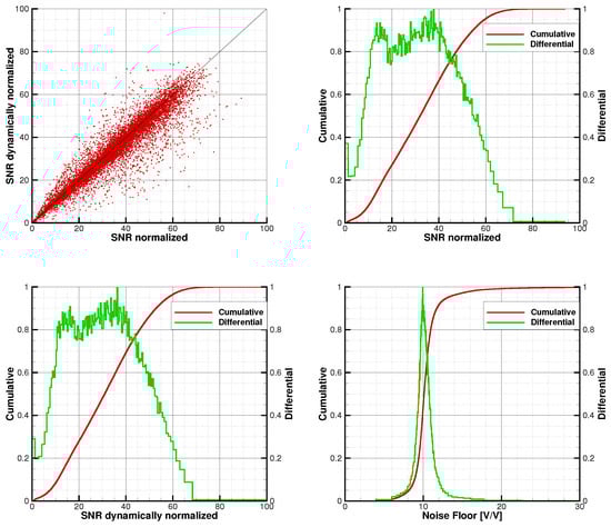
Figure 8.
SNR and noise floor statistics for Spire, GLONASS. Notation is the same as in Figure 1. GLONASS data indicate a stronger signal level and a narrower NF distribution as compared to GPS.
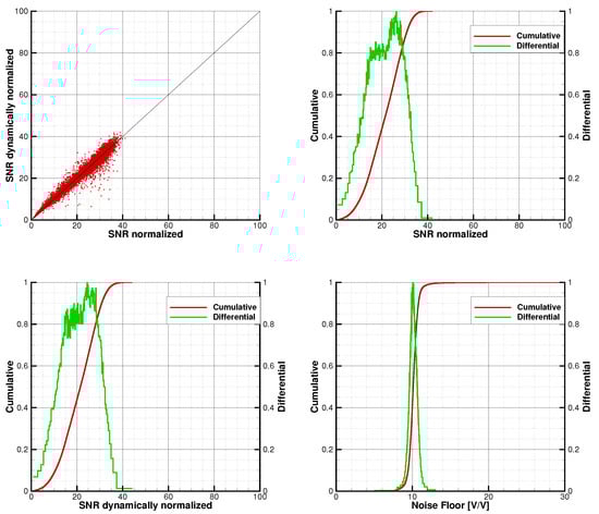
Figure 9.
SNR and noise floor statistics for Spire, Galileo. Notation is the same as in Figure 1.
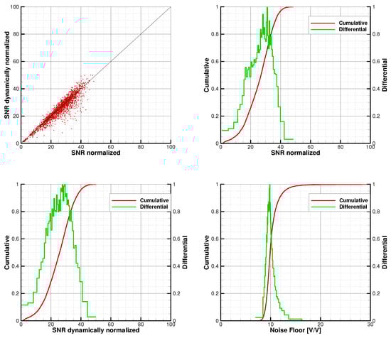
Figure 10.
SNR and noise floor statistics for Spire, QZSS. Notation is the same as in Figure 1.
The aforementioned feature of 2-D distributions conforms with the COSMIC-2 data, Figure 2 and Figure 3. Here, the NF distribution for GPS has a longer tail, as compared to GLONASS, where the distribution is sharper. The NF for GPS (18.4 V/V) is noticeably higher than that for GLONASS (14.6 V/V). Both values of NF are higher than that for COSMIC (GPS, 11.1 V/V). In addition, GLONASS produces a stronger signal, as compared to GPS.
The most complicated distributions are observed for the METOP missions. METOP-A (Figure 4) indicates a distribution of NF with two peaks (3.73 and 11.6 V/V). Here, we do not present the distributions for different latitude zones; however, we found that the peak at 3.73 is latitude dependent: it is strongest in the polar latitudes and it nearly disappears in the tropics. In fact, this peak does not correspond to real observation with low NF, it is a technical artifact. In this case, the signal in the shadow zone represents a series of short flashes. This corresponds to the upper cloud in the scatter plot of . The NF distribution has a long tail, which results in the specific structure of the lower cloud in the scatter plot.
METOP-B (Figure 5) indicates a bimodal distribution of NF, where the second mode corresponds to high values of NF. The second mode does not indicate a sharp peak, but it produces the lower cloud in the scatter plot of . METOP-C (Figure 6) combines the features of METOP-A and METOP-B: it has a weak secondary peak at low values of NF and also a third mode producing a long tail of the NF distribution and the lower cloud in the scatter plot. The main peaks of the NF distributions for all the three METOP missions lie close to each other at values 11.6, 12.0, and 11.8 V/V.
Spire data, shown in Figure 7, Figure 8, Figure 9 and Figure 10 are characterized by the lowest values of NF, which weakly depends on the GNSS constellation and varies from 9.64 to 10.1 V/V. The NF distributions are more narrow than for COSMIC, COSMIC-2, and METOP. Still, GPS produces the widest NF distribution. The signal strength conforms with what is observed for COSMIC-2: GLONASS produces a stronger signal as compared to GPS. Galileo and QZSS produce the weakest signal.
Table 1, Table 2, Table 3 and Table 4 show the most probable NF values, the median (), and the boundary () values for S, , and .

Table 1.
The most probable NF [V/V] for different missions and GNSS constellations.
Table 2.
The median () and boundary () of SNR [V/V] for different missions and GNSS constellations.
Table 3.
The median () and boundary () values of [unitless] for different missions and GNSS constellations.
Table 4.
The median () and boundary () values of [unitless] for different missions and GNSS constellations.
We conclude that is the most convenient measure of the signal intensity. It is normalized on the most probable value of NF, so its variability is generally smaller than that of . In separate events, the dynamic estimate of NF may be overevaluated, because the signal in the estimated shadow zone is always a sum of the noise, deep RO signals, interference from other satellites, etc. It is the distributions that reveal the true value of the noise floor.
4. Conclusions
In this study, we investigated the statistics of the average SNR at altitudes 60–80 km and the statistics of the NF for different missions (COSMIC, METOP-A,B,C, COSMIC-2, and Spire) for different constellations (GPS, GLONASS, Galileo, and QZSS). We processed large arrays of RO observations, from about 60,000 to about 300,000 per mission. The QC was reduced to a minimum: it was only requested that the specified characteristics of the SNR record were possible to be evaluated. We estimated the 1-D distributions of NF, for which we evaluated the most probable values. It was shown that the NF distributions always have a main sharp peak. The most probable value of NF was found to be the lowest for the 3U nanosatellite mission Spire, where NF is about 10 V/V for all the GNSS constellations. COSMIC and METOP have slightly higher values of NF, which are about 11–12 V/V. COSMIC-2 indicates the highest NF, which noticeably differs for GPS (18.4 V/V) and for GLONASS (14.6 V/V). This, however, may only be dependent on the different normalization levels used for the definition of the V/V unit, rather than on the real noise levels.
Using the values of NF, which can be both dynamical, i.e., evaluated for the specific RO event, and most probable, i.e., evaluated from the distribution for the specific mission and constellation, it is possible to define two normalizations of the SNR: (1) dynamically normalized, which is defined as the ratio of SNR in V/V and the dynamic NF, and (2) normalized, the ratio of SNR and the most probably NF.
METOP indicates the most complicated multimodal distributions of NF. In particular, METOP-A has a fraction of events with a low NF (3.73 V/V). On the other hand, METOP-B and METOP-C have a long tail in the NF distribution. A general observation is that the distributions have the most complicated structure for the GPS constellation.
The definitions of normalized and dynamically normalized SNR provide the basis for the follow-on study of the comparison of the inversion characteristics for different missions and constellations as function of the SNR.
Author Contributions
Conceptualization, M.G., V.I. and C.R.; methodology, M.G.; software, M.G. All authors have read and agreed to the published version of the manuscript.
Funding
This study was funded by the Russian Foundation for Basic Research, grant No. 20-05-00189 A.
Institutional Review Board Statement
Not applicable.
Informed Consent Statement
Not applicable.
Data Availability Statement
The COSMIC, METOP, and COSMIC2 data used in this study are freely available at CDAAC Web-site. The Spire data used in this study are only distributed on a commercial basis or provided in framework of special agreements.
Acknowledgments
The authors acknowledge Taiwan’s National Space Organization (NSPO) and the University Corporation for Atmospheric Research (UCAR) for providing the COSMIC and COSMIC-2 Data. The authors are grateful to Rob Kursinski and other reviewers of the previous version of the paper for their valuable criticism.
Conflicts of Interest
The authors declare no conflict of interest.
Abbreviations
The following abbreviations are used in this manuscript:
| CDAAC | COSMIC Data Analysis and Archive Center |
| CICERO | Community Initiative for Cellular Earth Remote Observation |
| COSMIC | Constellation Observing System for Meteorology, Ionosphere, and Climate |
| EUMETSAT | European Organisation for the Exploitation of Meteorological Satellites |
| GLONASS | Global Navigation Satellite System (Russian navigation system) |
| GNSS | Global Navigation Satellite System |
| GO | Geometrical Optics |
| GPS | Global Positioning System |
| METOP | Meteorological Operational Satellite |
| MSISE | Mass-Spectrometer-Incoherent-Scatter model Extended |
| NF | Noise Floor |
| PBL | Planetary Boundary Layer |
| Probability Distribution Function | |
| RMS | Root-Mean-Square |
| QC | Quality Control |
| QZSS | Quasi-Zenith Satellite System |
| RO | Radio Occultation |
| SNR | Signal-to-Noise Ratio |
| WO | Wave Optics |
References
- Sokolovskiy, S.; Schreiner, W.; Weiss, J.; Zeng, Z.; Hunt, D.; Braun, J. Initial Assessment of COSMIC-2 Data in the Lower Troposphere. In Proceedings of the Joint 6th ROM SAF Data User Workshop and 7th IROWG Workshop, Elsinore, Denmark, 19–25 September 2019. [Google Scholar]
- Schreiner, W.S.; Weiss, J.P.; Anthes, R.A.; Braun, J.; Chu, V.; Fong, J.; Hunt, D.; Kuo, Y.H.; Meehan, T.; Serafino, W.; et al. COSMIC-2 Radio Occultation Constellation: First Results. Geophys. Res. Lett. 2020, 47, e2019GL086841. [Google Scholar] [CrossRef]
- Ho, S.P.; Zhou, X.; Shao, X.; Zhang, B.; Adhikari, L.; Kireev, S.; He, Y.; Yoe, J.G.; Xia-Serafino, W.; Lynch, E. Initial Assessment of the COSMIC-2/FORMOSAT-7 Neutral Atmosphere Data Quality in NESDIS/STAR Using In Situ and Satellite Data. Remote Sens. 2020, 12, 4099. [Google Scholar] [CrossRef]
- Lin, C.Y.; Lin, C.C.H.; Liu, J.Y.; Rajesh, P.K.; Matsuo, T.; Chou, M.Y.; Tsai, H.F.; Yeh, W.H. The Early Results and Validation of FORMOSAT-7/COSMIC-2 Space Weather Products: Global Ionospheric Specification and Ne-Aided Abel Electron Density Profile. J. Geophys. Res. Space Phys. 2020, 125, e2020JA028028. [Google Scholar] [CrossRef]
- Bonnedal, M.; Christensen, J.; Carlström, A.; Berg, A. Metop-GRAS in-orbit instrument performance. GPS Solut. 2010, 14, 109–120. [Google Scholar] [CrossRef]
- Schreiner, W.; Sokolovskiy, S.; Hunt, D.; Rocken, C.; Kuo, Y.H. Analysis of GPS radio occultation data from the FORMOSAT-3/COSMIC and Metop/GRAS missions at CDAAC. Atmos. Meas. Tech. 2011, 4, 2255–2272. [Google Scholar] [CrossRef]
- Von Engeln, A.; Andres, Y.; Marquardt, C.; Sancho, F. GRAS radio occultation on-board of Metop. Adv. Space Res. 2011, 47, 336–347. [Google Scholar] [CrossRef]
- Hsieh, M.E.; Chen, Y.-C.; Hsiao, L.F.; Chang., L.-Y.; Huang, C.Y. Case Study of Impact of Assimilating MetOp GPS Radio Occultation Observation on Top of COSMIC Data on Typhoon Forecast. J. Aeronaut. Astrnaut. Aviat. 2018, 50, 375–390. [Google Scholar] [CrossRef]
- Rapp, M.; Dörnbrack, A.; Kaifler, B. An intercomparison of stratospheric gravity wave potential energy densities from METOP GPS radio occultation measurements and ECMWF model data. Atmos. Meas. Tech. 2018, 11, 1031–1048. [Google Scholar] [CrossRef]
- Irisov, V.; Duly, T.; Nguyen, V.; Masters, D.; Correig, O.N.; Tan, L.; Yuasa, T.; Ector, D. Recent radio occultation profile results obtained from Spire CubeSat GNSS-RO constellation. In Proceedings of the AGU Fall Meeting, Washington, DC, USA, 10–14 December 2018. [Google Scholar]
- Irisov, V.; Ector, D.; Duly, T.; Nguyen, V.; Nogues-Correig, O.; Tan, L.; Yuasa, T. Atmospheric Radio Occultation Observation from Spire CubeSat Nanosatellites. In Proceedings of the AMS Annual Meeting, Washington, DC, USA, 10–14 December 2018. [Google Scholar]
- Gorbunov, M.; Koval, O.; Kirchengast, G. Kirkwood Distribution Function and its Application for the Analysis of Radio Occultation Observations. In Proceedings of the Joint 6th ROM SAF User Workshop and 7th IROWG Workshop, EUMETSAT ROM SAF, Elsinore, Denmark, 19–25 September 2019. [Google Scholar]
- Irisov, V.; Nguyen, V.; Duly, T.; Nogues-Correig, O.; Tan, L.; Yuasa, T.; Masters, D.; Sikarin, R.; Gorbunov, M.; Rocken, C. Radio Occultation Observations and Processing from Spire’s CubeSat Constellation. In Proceedings of the Joint 6th ROM SAF User Workshop and 7th IROWG Workshop, EUMETSAT ROM SAF, Elsinore, Denmark, 19–25 September 2019. [Google Scholar]
- Bowler, N.E. An assessment of GNSS radio occultationdata produced by Spire. Q. J. R. Meteorol. Soc. 2020, 146, 3772–3788. [Google Scholar] [CrossRef]
- Kursinski, E.R. Weather & Space Weather RO Data from PlanetiQ Commercial GNSS RO. In Proceedings of the Joint 6th ROM SAF Data User Workshop and 7th IROWG Workshop, Elsinore, Denmark, 19–25 September 2019. [Google Scholar]
- Chang, H.; Lee, J.; Wang, Y.; Breitsch, B.; Morton, Y.J. Preliminary Assessment of CICERO Radio Occultation Performance by Comparing with COSMIC I Data. In Proceedings of the 33rd International Technical Meeting of the Satellite Division of The Institute of Navigation, Online, 21–25 September 2020. [Google Scholar] [CrossRef]
- Sokolovskiy, S.; Schreiner, W.; Zeng, Z.; Hunt, D.; Lin, Y.C.; Kuo, Y.H. Observation, analysis, and modeling of deep radio occultation signals: Effects of tropospheric ducts and interfering signals. Radio Sci. 2014, 49, 954–970. [Google Scholar] [CrossRef]
- Sokolovskiy, S.; Rocken, C.; Schreiner, W.; Hunt, D. On the uncertainty of radio occultation inversions in the lower troposphere. J. Geophys. Res. 2010, 115, D22111. [Google Scholar] [CrossRef]
- Sokolovskiy, S.; Rocken, C.; Hunt, D.; Schreiner, W.; Johnson, J.; Masters, D.; Esterhuizen, S. GPS profiling of the lower troposphere from space: Inversion and demodulation of the open-loop radio occultation signals. Geophys. Res. Lett. 2006, 33, L14816. [Google Scholar] [CrossRef]
- Gorbunov, M.E.; Lauritsen, K.B. Analysis of wave fields by Fourier integral operators and its application for radio occultations. Radio Sci. 2004, 39, RS4010. [Google Scholar] [CrossRef]
- Jensen, A.S.; Lohmann, M.S.; Nielsen, A.S.; Benzon, H.H. Geometrical optics phase matching of radio occultation signals. Radio Sci. 2004, 39, RS3009. [Google Scholar] [CrossRef]
- Gorbunov, M.; Kirchengast, G.; Lauritsen, K.B. Generalized canonical transform method for radio occultation sounding with improved retrieval in the presence of horizontal gradients. Atmos. Meas. Tech. 2021, 14, 853–867. [Google Scholar] [CrossRef]
- Hedin, A.E. Extension of MSIS thermosphere model into the middle and lower atmosphere. J. Geophys. Res. 1991, 96, 1159–1172. [Google Scholar] [CrossRef]
- Sokolovskiy, S.V. Modeling and inverting radio occultation signals in the moist troposphere. Radio Sci. 2001, 36, 441–458. [Google Scholar] [CrossRef]
- Gorbunov, M.E.; Sokolovskiy, S.V. Remote Sensing of Refractivity from Space for Global Observations of Atmospheric Parameters; Report 119; Max–Planck Institute for Meteorology: Hamburg, Germany, 1993; 58p. [Google Scholar]
- Scherllin-Pirscher, B.; Syndergaard, S.; Foelsche, U.; Lauritsen, K.B. Generation of a bending angle radio occultation climatology (BAROCLIM) and its use in radio occultation retrievals. Atmos. Meas. Tech. 2015, 8, 109–124. [Google Scholar] [CrossRef][Green Version]
- Gorbunov, M.E.; Shmakov, A.V. Statistically average atmospheric bending angle model based on COSMIC experimental data. Izv. Atmos. Oceanic Phys. 2016, 52, 622–628. [Google Scholar] [CrossRef]
- Beyerle, G.; Gorbunov, M.E.; Ao, C.O. Simulation studies of GPS radio occultation measurements. Radio Sci. 2003, 38, 1084. [Google Scholar] [CrossRef]
- Gorbunov, M.E.; Gurvich, A.S.; Shmakov, A.V. Back-propagation and radio-holographic methods for investigation of sporadic ionospheric E-layers from Microlab-1 data. Int. J. Remote Sens. 2002, 23, 675–685. [Google Scholar] [CrossRef]
- Sokolovskiy, S.V.; Schreiner, W.; Rocken, C.; Hunt, D. Detection of high-altitude ionospheric irregularities with GPS/MET. Geophys. Res. Let. 2002, 29, 3-1–3-4. [Google Scholar] [CrossRef]
- Kuo, Y.H.; Wee, T.K.; Sokolovskiy, S.; Rocken, C.; Schreiner, W.; Hunt, D.; Anthes, R.A. Inversion and Error Estimation of GPS Radio Occultation Data. J. Meteorolog. Soc. Jpn. 2004, 82, 507–531. [Google Scholar] [CrossRef]
- Syndergaard, S. Modeling the impact of the Earth’s oblateness on the retrieval of temperature and pressure profiles from limb sounding. J. Atmos. Sol. Terr. Phys. 1998, 60, 171–180. [Google Scholar] [CrossRef]
- Xiaohua, X.; Zhenghang, L.; Jia, L. Correction on effect of Earth’s oblateness in inversion of GPS occultation data. Geo Spat. Inform. Sci. 2005, 8, 247–250. [Google Scholar] [CrossRef][Green Version]
Publisher’s Note: MDPI stays neutral with regard to jurisdictional claims in published maps and institutional affiliations. |
© 2022 by the authors. Licensee MDPI, Basel, Switzerland. This article is an open access article distributed under the terms and conditions of the Creative Commons Attribution (CC BY) license (https://creativecommons.org/licenses/by/4.0/).