Article

High-Precision Source Positions Obtained by the Combined Inversion of Different-Order Local Wavenumbers Derived from Aeromagnetic Data

1
College of Geo-Exploration Sciences and Technology, Jilin University, Changchun 130026, China
2
Key Laboratory of Geophysical Exploration Equipment Ministry of Education of China, Jilin University, Changchun 130026, China
3
Institute of National Development and Security Studies, Jilin University, Changchun 130026, China
*
Author to whom correspondence should be addressed.
Remote Sens. 2022, 14(3), 591; https://doi.org/10.3390/rs14030591
Submission received: 27 November 2021 / Revised: 16 January 2022 / Accepted: 25 January 2022 / Published: 26 January 2022

Abstract

:
The aeromagnetic survey is a common remote sensing tool for detecting iron deposits. The local wavenumber of a magnetic anomaly is used to interpret the edges or positions of the sources, and can involve first- or second-order local wavenumbers. In this paper, we derived a linear equation between the second-order local wavenumber and the source location; therefore, we propose a constraint of first and second-order local wavenumbers. Tests on synthetic data show that the source parameters, computed using a combination of equations that involved different-order local wavenumbers, are closer to the true values and show a smaller spread in estimated values. For gridded data, we proved that the different-order combination allowed us to accurately estimate the source position. When applied to the aeromagnetic data from Hebei province, China, we refined the location of most magnetic features, which we interpreted as possible iron deposits.

Graphical Abstract

1. Introduction

Aero-magnetism is an important remote measurement method for resource exploration [1] in construction, mining and archaeology. One of the main aeromagnetic survey platforms is unmanned aircraft [2]. A complex environmental interpretation system is proposed to perform a quantitative analysis of observed anomalies and a comprehensive examination. [3] Amin used a magnetic survey and DC resistivity in a multi-scale approach to study the characteristics and image cases of various archaeological assets in a highly terraneous site [4]. From a series of aeromagnetic data images in South China, a detailed construction of the South China block was revealed [5]. It is helpful to study the intracontinental tectonic evolution in this area.
Ferromagnetic ore bodies generally exhibit high-value anomalies, so, aero-magnetism is the most widely used technique for finding ore bodies with this characteristic. Extracting the magnetite-caused anomalies from the aeromagnetic data can lead to a preliminary estimation of magnetite prospective resources [6]. James delineated mineral targets or potential zones using high-resolution aeromagnetic data [7]. Sayed performed an aeromagnetic data analysis to locate probable mineral deposits in the southeastern desert of Egypt [8].
Field source location acquisition is the basic task of aeromagnetic data interpretation, for which there are many techniques, such as the Werner deconvolution, Euler deconvolution, analytic signal, source parameter imaging, and local wavenumber [9,10,11,12,13,14]. The local wavenumber was defined by Thurston and Smith as the first horizontal derivative of the local phase and is independent of magnetization direction, so it is often used to compute the distribution of magnetic source [13,15]. Smith directly estimated the source depth and structural index by using the ratio of first- and second-order local wavenumbers [16]. The depth and the nature of the sources can be estimated simultaneously by using an improved local wavenumber technique [17]. A linear equation composed of vertical and horizontal local wavenumbers can obtain source location information, which is the enhanced local wavenumber method [14]. Keating used the local wavenumbers and their vertical derivatives to estimate the source location without a priori knowledge of the geological body type [18]. Abbas dealt with the local wavenumber method and estimated the depth and the structural index [19]. The fast local wavenumber (FLW) technique used the sum of the square of the vertical and horizontal local wavenumbers to establish a new linear equation that could simultaneously estimate the source location and structural index [20].
In our research, we investigated different combinations of equations with multiple-order local wavenumbers to obtain more precise location parameters. Model tests were carried out on point sources, line sources and contact strips to verify the method. Similar combinations and a profile combination applied perpendicular to the strike were tested on aeromagnetic data.

2. Different-Order Local Wavenumber Method

2.1. 2D Local Wavenumber Method

The first-order local wavenumbers are the first derivatives of the local phase (θ) [13,14,15], and can be expressed as:
k x = θ x = x [ tan 1 ( f / z f / x ) ] = 1 A 2 ( 2 f x z f x 2 f x 2 f z )
k z = θ z = z [ tan 1 ( f / z f / x ) ] = 1 A 2 ( 2 f x z f z 2 f z 2 f x )
where, kx and kz are the horizontal and vertical local wavenumbers of magnetic anomaly f, respectively, and A = ( f z ) 2 + ( f x ) 2 , is the analytic signal amplitude of f. The vertical derivatives in the formula adopt the frequency domain method, and the horizontal derivatives adopt the difference quotient method in the space domain.
Smith and Salem derived the analytic expressions of first-order local wavenumbers, which can be given by [17]:
k x = ( N + 1 ) ( z 0 z ) ( x x 0 ) 2 + ( z z 0 ) 2
k z = ( N + 1 ) ( z 0 z ) ( x x 0 ) 2 + ( z z 0 ) 2
where (x0, z0) is the coordinate of the source, (x, z) is the coordinate of the observation point, and N is the structural index, which represents the shape of the source.
Salem first built a linear equation between the first-order local wavenumbers and source location to compute the location parameters (x0, z0) of the source [14]. The first-order local wavenumber estimator A (estimator A1) is given by:
k x ( x x 0 ) + k z ( z z 0 ) = 0
A window of multiple adjacent (x, z) points and corresponding wavenumbers are used to generate many versions of this equation, which can be solved in a least squares manner to estimate the x0 and z0 on the assumption that they are all influenced by the same nearby source. The multiple points are called a data window.
Ma gave another linear equation based on a different combination of the first-order local wavenumbers that could similarly estimate the structural index and source location [21]. The first-order local wavenumber estimator B (estimator B1) is given by:
k z ( x x 0 ) + k x ( z 0 z ) = N + 1
Smith defined the second-order local wavenumbers as the derivative of the ratio of the second-order vertical derivative to the horizontal derivative [16].
k 2 x = θ x = x tan 1 [ 2 f / 2 z 2 f / ( x z ) ] = 3 f z 2 x 2 f x z 2 f z 2 3 f z x 2 ( 2 f x z ) 2 + ( 2 f x 2 ) 2 = ( N + 2 ) ( z 0 z ) ( x x 0 ) 2 + ( z z 0 ) 2 .
k 2 z = θ z = z tan 1 [ 2 f / 2 z 2 f / ( x z ) ] = 3 f x 2 z 2 f x z 2 f x 2 3 f x z 2 ( 2 f x z ) 2 + ( 2 f x 2 ) 2 = ( N + 2 ) ( x x 0 ) ( x x 0 ) 2 + ( z z 0 ) 2 .
Linear equations involving second-order local wavenumbers and the source location (the detailed derivation is given in the Appendix A) are named second-order local wavenumber estimators A and B (estimator A2 and estimator B2), which can be expressed as:
k 2 x ( x x 0 ) + k 2 z ( z z 0 ) = 0
k 2 z ( x x 0 ) + k 2 x ( z 0 z ) = N + 2
Those equations can also be used to obtain the location of the source and the structural index using data windows and a least squares approach.
From first- and second-order local wavenumber estimators, we see that the different-order local wavenumbers can be used to compute the source parameters. We investigated whether using different combinations of multiple-order local wavenumbers could return more accurate results.
There are also three combinations that involve wavenumbers with different orders.
The different-order local wavenumber estimator A (estimator Ad) composed of estimator A1 and estimator A2 is:
[ k x , k z k 2 x , k 2 z ] [ x 0 z 0 ] = [ k x x + k z z k 2 x x + k 2 z z ] .
The different-order local wavenumber estimator B (estimator Bd) composed of estimator B1 and estimator B2 is:
[ k z , k x , 1 k 2 z , k 2 x , 1 ] [ x 0 z 0 N ] = [ k z x k x z 1 k 2 z x k 2 x z 2 ] .
The different-order local wavenumber estimator D (estimator Dd) composed of the estimator A1, estimator B1, estimator A2 and estimator B2 is:
[ k x , k z , 0 k 2 x , k 2 z , 0 k z , k x , 1 k 2 z , k 2 x , 1 ] [ x 0 z 0 N ] = [ k x x + k z z k 2 x x + k 2 z z k z x k x z 1 k 2 z x k 2 x z 2 ] .
Note that the combination in estimator Ad, can only be used to determine the location, but estimator Bd and estimator Dd can also be used to determine the structural index.
Similarly, there are combinations that involve the same-order local wavenumbers that we can use to compare the results.
The same-order local wavenumber estimator A (estimator As) composed of estimator A1 and estimator B1 is:
[ k x , k z , 0 k z , k x , 1 ] [ x 0 z 0 N ] = [ k x x + k z z k z x k x z 1 ] .
The same-order local wavenumber estimator B (estimator Bs) composed of the estimator A2 and estimator B2 is:
[ k 2 x , k 2 z , 0 k 2 z , k 2 x , 1 ] [ x 0 z 0 N ] = [ k 2 x x + k 2 z z k 2 z x k 2 z x 2 ] .

2.2. 3D Local Wavenumber Method

These equations are based on 2D geometry and are best applied along profiles perpendicular to the geological strike. For 3D situations, the following equations better apply. The three-dimensional forms of the estimator A1 and estimator A2 can be written:
k x ( x x 0 ) + k y ( y y 0 ) + k z ( z z 0 ) = 0 ,
k 2 x ( x x 0 ) + k 2 y ( y y 0 ) + k 2 z ( z z 0 ) = 0 .
We named Equation (16) as the first-order local wavenumber estimator C (estimator C1), in reference to Salem [22], and Equation (17) is a second-order local wavenumber estimator C (estimator C2), which is presented in Appendix B.
The three-dimensional form of the different-order local wavenumber estimator C (estimator Cd) can be expressed as:
[ k x , k y , k z k 2 x , k 2 y , k 2 z ] [ x 0 y 0 z 0 ] = [ k x x + k y y + k z z k 2 x x + k 2 y y + k 2 z z ] .
In the following, we test the different equations and combinations on synthetic data with and without noise corruption. Spurious solutions will be accepted or rejected based on the following procedure:
  • Using a small solution space window to assess isolated solutions. If the distance between the point and all other points belonging to a cluster is less than the threshold but not more than the sampling interval, then the point belongs to the cluster;
  • Fusing or joining clusters if the horizontal centers are less than the root square of 10% with the position of the center;
  • Finally, eliminating a cluster if it has fewer than a given number of solutions because clusters with a small number of points are not statistically important.

3. Experiments and Results

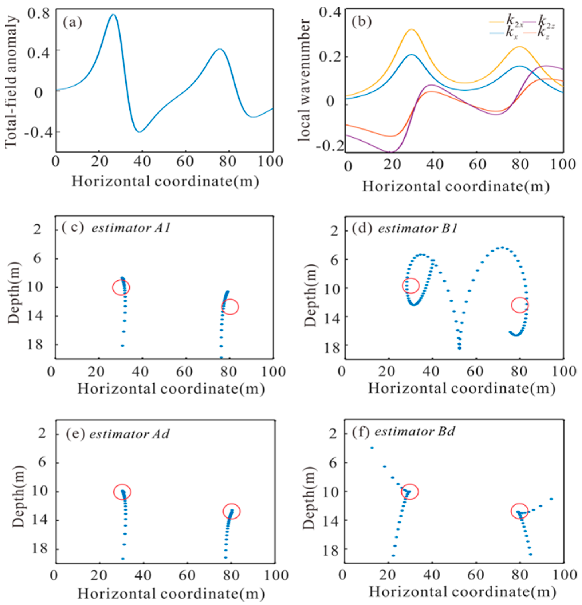
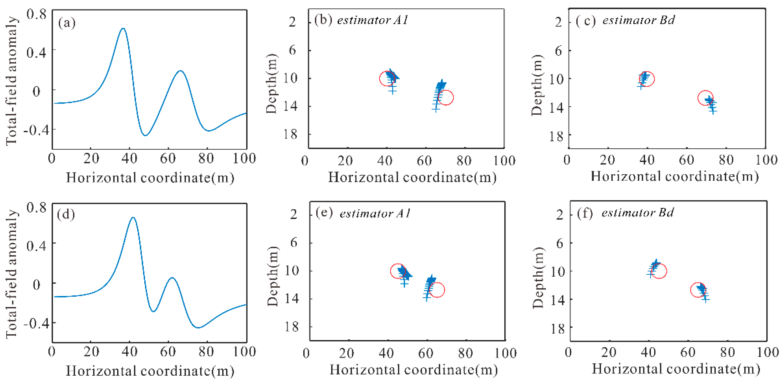
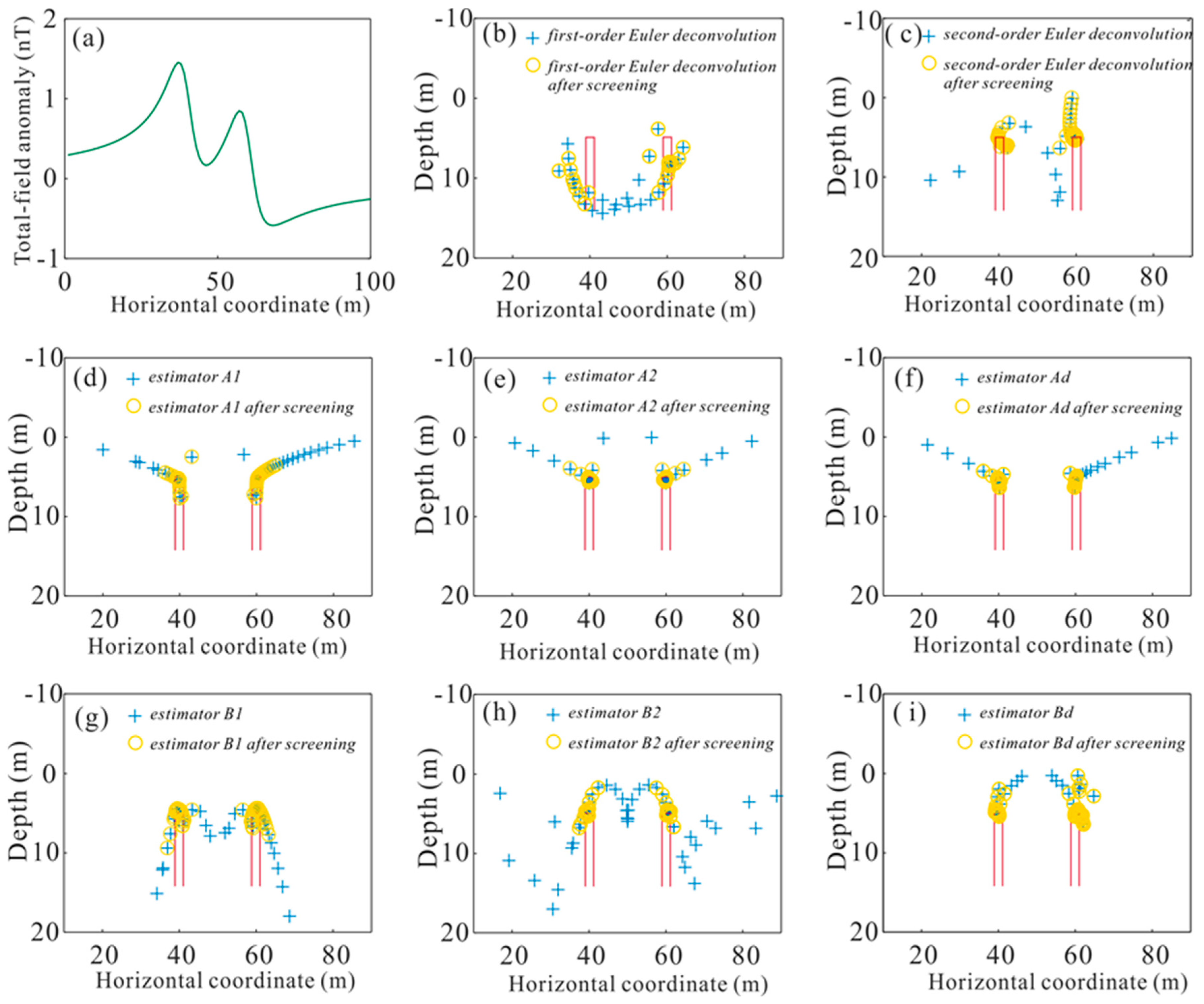
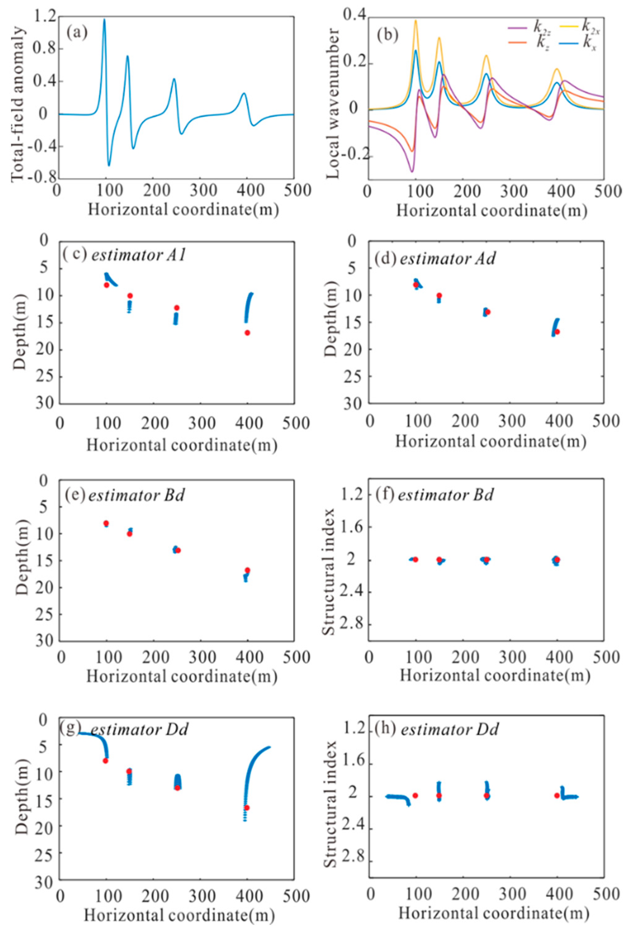
3.1. 2D Theoretical Model

We tested different combinations of the above equations on the magnetic anomalies of two adjacent horizontal cylindrical geological bodies that had horizontal coordinates (x0) of 30 and 80 m, depths (z0) of 10 and 13 m, and radii of 7 m. Figure 1a shows magnetic anomalies with an inclination of 60° and a declination perpendicular to the strike magnetization 1 A/m. Figure 1b shows the associated first- and second-order local wavenumbers. The point spacing in the theoretical model tests was 5. The number of the data window was 11. The selection of the window size is related to the size and distribution of the target geological bodies. A small window will lead to inaccuracy and the divergence of the calculation results. Moreover, one window contains information of, at most, one field source, which can avoid the interference of nearby field sources to a certain extent. According to the above reasons, the window size should be more than twice the length of the line or point spacing [23].
Figure 1c,d are the source locations calculated using estimators A1 and B1. The true locations of the cylinders are labeled by red circles, and the estimated results are labeled by blue crosses, each representing a different location derived from a different data window. The depths are shallower than the actual values and showed some scattered points. Figure 1e,f show estimated depths using estimators Ad and Bd without screening. They show accurate but scattered source locations, which are less conducive to interpretation.
To obtain a more accurate estimate of the geological body position, the results were screened, and the number set to 10. Figure 2a presents the source locations based on calculations using estimator A1. The depths were obviously slightly shallower than the actual depths, and they show a moderate spread of positions. Figure 2b,c show the source locations and the structural index, respectively, calculated using estimator B1. After screening, the results showed a significant spread. Figure 2d–f show the source depths and the structural index calculated using the estimators A2 and B2. The spread is similar to Figure 2a–c, so we concluded that a single equation composed only of first- or only of second-order local wavenumbers could not generate accurate source locations for magnetic anomalies of multiple anomalous bodies. Figure 2g represents the source location results calculated using estimator Ad. The horizontal locations were consistent with the true location, and the mean depths were 9.7 and 12.7 m, which were close to the actual depths. Figure 2h,i show the source depths and the structural index calculated using the estimator Bd. These inversion results were also very close to the true values and gave an accurate structural index. Figure 2j,k show the source locations and structural index calculated using estimator Dd, which is a combination of estimators A1, B1, A2 and B2. They contain first- and second-order local wavenumbers and the results showed some scattering. Figure 2l,m show the source locations and structural index results calculated using estimator As. There is a combination of only first-order local wavenumbers, and the estimated depths were close to the actual values, but the structural index showed significant scatter. The source depths and structural index calculated using estimator Bs (a combination of only second-order local wavenumbers) are shown in Figure 2n,o, and the structural index had large scattering. The best results were obtained using estimator Ad, but only if we wished to calculate the source position. Estimator Bd was used to calculate the position and structural index because of the corresponding consistent relationship between the same-order local wavenumbers and the geological body.
To further test the ability of our method to divide the spatial location of adjacent geological bodies, we gradually reduced the location between the above two horizontal cylinders and compared the results obtained with estimator A1 and estimator Bd, respectively. Figure 3a shows that the magnetic anomalies with horizontal coordinates (x0) were 40 and 70 m. Figure 3b,c show the results generated by estimator A1 and estimator Bd. There was a certain deviation between the results of estimator A1 and the actual depths, but estimator Bd restored the spatial position of the geological body. When the distance between two horizontal cylinders is reduced to 20 m, the magnetic anomalies with horizontal coordinates (x0) were 45 and 65 m, as shown in Figure 3d. Figure 3e is the result calculated by estimator A1. At this time, the estimator was still unable to obtain the vertical distribution of adjacent geological bodies, but estimator Bd gave results consistent with the actual situation.
To take the local wavenumber method and Euler deconvolution [10] comparison further, we defined two infinite vertical sheets having a 60° inclination and a 1 A/m magnetization magnetic anomaly having horizontal positions 40 and 60 m, a depth of 5 m, and a width of 0.2 m, as shown in Figure 4a. The number of the data window was 11. Figure 4b presents the result determined by first-order Euler deconvolution, which cannot define the source locations in either the horizontal or vertical direction. The real position is indicated by the red area in the figure. The yellow circle marks the results after screening, the cluster number of the screening is 10, and the blue plus sign marks the unprocessed results. Figure 4c shows the source locations calculated by second-order Euler deconvolution, and the results show some scattering.
Figure 4d,g show the scattered source locations using estimators A1 and B1 without noise and filter. Then, we chose estimators A2 and B2 to calculate the source locations. The results were accurate (Figure 4e,h). The source locations determined by estimator Ad and Bd without a filter are shown in Figure 4f,i, in the last four cases (Figure 4e,h,f,i), the source location results were close to the actual values.
Because the source imaging method uses the derivatives of the field, which are more sensitive to noise, we used noise-corrupted magnetic anomalies with a Gaussian filter to determine the source information. As for real potential-field data, a filter was also needed. To test these two combinations’ robustness to noise, Figure 5a shows the noise-free magnetic anomaly, the noise-corrupted anomaly with Gaussian noise of 1% and the same noise-corrupted magnetic anomaly after applying the Gaussian filter (the variance is 0.3 nT). Although noise has a great influence on anomalies, we applied Laplace’s equation [24] when solving the derivative; the vertical derivative was calculated from a combination of the horizontal derivatives. In this way, the amplification of noise can be reduced to a certain extent. Figure 5b,c present the results determined by first- and second-order Euler deconvolution, the results show scatter and low horizontal resolution. The results, based on model calculations using estimator A1 and A2 after filtering, are shown in Figure 5d,e and exhibit large differences between the estimated results and actual values. Figure 5f shows the source depths calculated using the estimator Ad; the inversion results after filtering were close to the true values.
We then increased the amplitude of the noise to test the performance of different local wavenumber estimators. Figure 5g shows the noise-free magnetic anomaly, noise-corrupted magnetic anomaly with Gaussian noise of 3%, and the same noise-corrupted magnetic anomaly after a Gaussian filter. The model results generated using first-order Euler deconvolution are shown in Figure 5h, and exhibit a large error with respect to the actual values. We obtained source locations using second-order Euler deconvolution (Figure 5i) with a low horizontal resolution. Figure 5j,k,l are the source locations determined by estimators A1, A2 and Ad, and the distribution of the results obviously became more scattered as the noise increased, but we roughly determined the source positions by estimator A1. The root mean square (RMS) between the true depths and the estimated source depths determined by estimator A1, A2 and Ad are shown in Figure 5m, so that for high-resolution data, the combinations of the local wavenumber improved the horizontal and vertical resolution of the results.
To further understand the efficacy of estimators A1, Ad and Bd, we designed a more complicated anomaly of four horizontal cylinders with coordinates (x0, z0): (100, 8 m), (150, 10 m), (250, 13 m), and (400, 17 m). The total-field magnetic anomaly with a magnetization inclined at 60°, and the first- and second-order local wavenumbers, are shown in Figure 6a,b. Note that we made the deeper cylinders further from the near cylinders to reduce the impact of interference. The point spacing in theoretical model tests is 3. The number of the data window was 7.
Figure 6c shows the source locations calculated using estimator A1. The true location is labeled by a red circle in the figure. This result shows that calculating the source depths with a single equation of local wavenumbers will not yield accurate results for multiple geological bodies. Figure 6d presents the source depths based on calculations using estimator Ad; Figure 6e,f show the source depths and the structural index results using estimator Bd, and accurate results with low scattering were evident. The model results generated using estimator Dd were not close to the actual values (Figure 6g,h). Based on these case studies, we saw that the previously identified combinations of local wavenumbers (estimator Ad and Bd) still had good performance on multiple anomalous bodies.

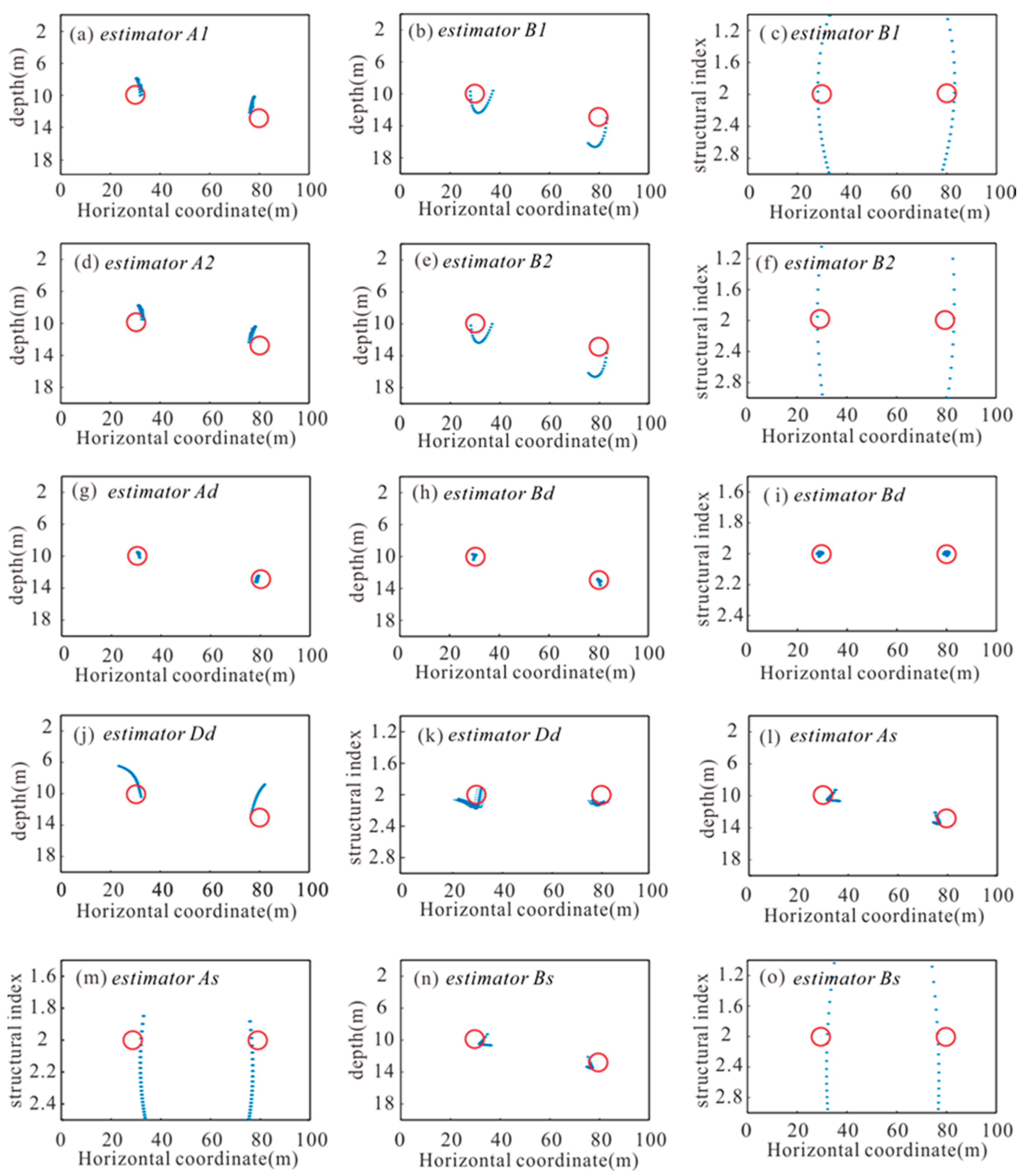
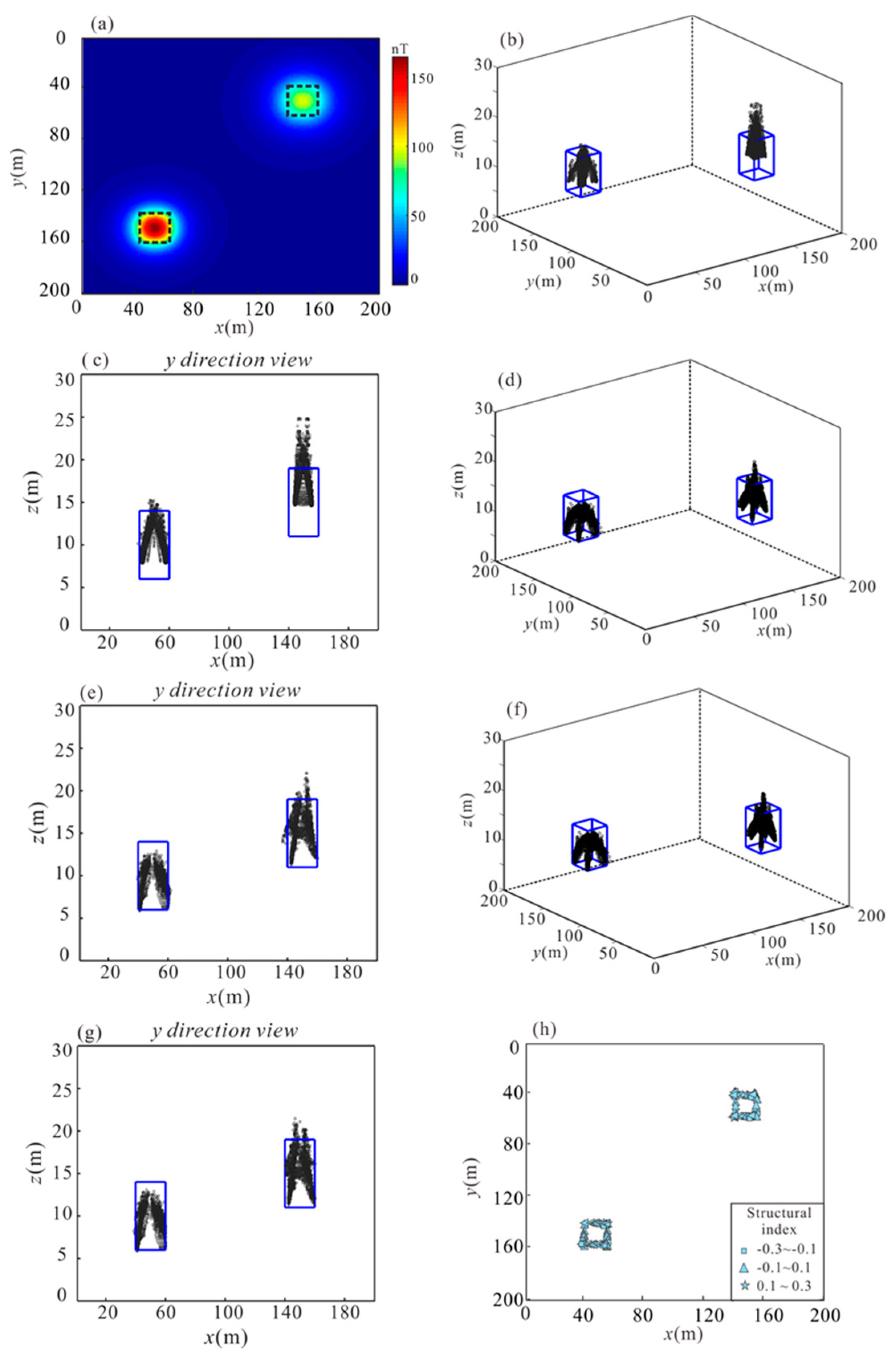
3.2. 3D Theoretical Model

For 3D situations, we obtained the (x0, y0, z0) using estimators C1, C2 and Cd. Because estimator Bd did not have a corresponding three-dimensional form, we generally calculated the derivative of the gridded data in the direction perpendicular to the strike, and then used estimator Bd to compute the source location (x0, y0, z0) and structural index for the gridded data. The same two-dimensional methodology for the inversion of gridded data was also used in other methods [13,16]. Figure 7a shows the gridded magnetic anomaly of two rectangular prisms at 6 and 11 m top buried depths, and the horizontal locations of the prisms were marked by black outlines. The point spacing in the theoretical model tests was 5. The number of the data window was 11.
The locations generated using only estimator C1 are shown in Figure 7b,c, and there was a large deviation between the results and the actual values. Figure 7d,e show the locations and depths computed by estimator Cd. Figure 7f–h are the positions and structural index computed by the estimator Bd. The results showed that the combination of different-order local wavenumbers gave more accurate results, the depths were closer to real values, and the structural index values were basically zero, as expected.

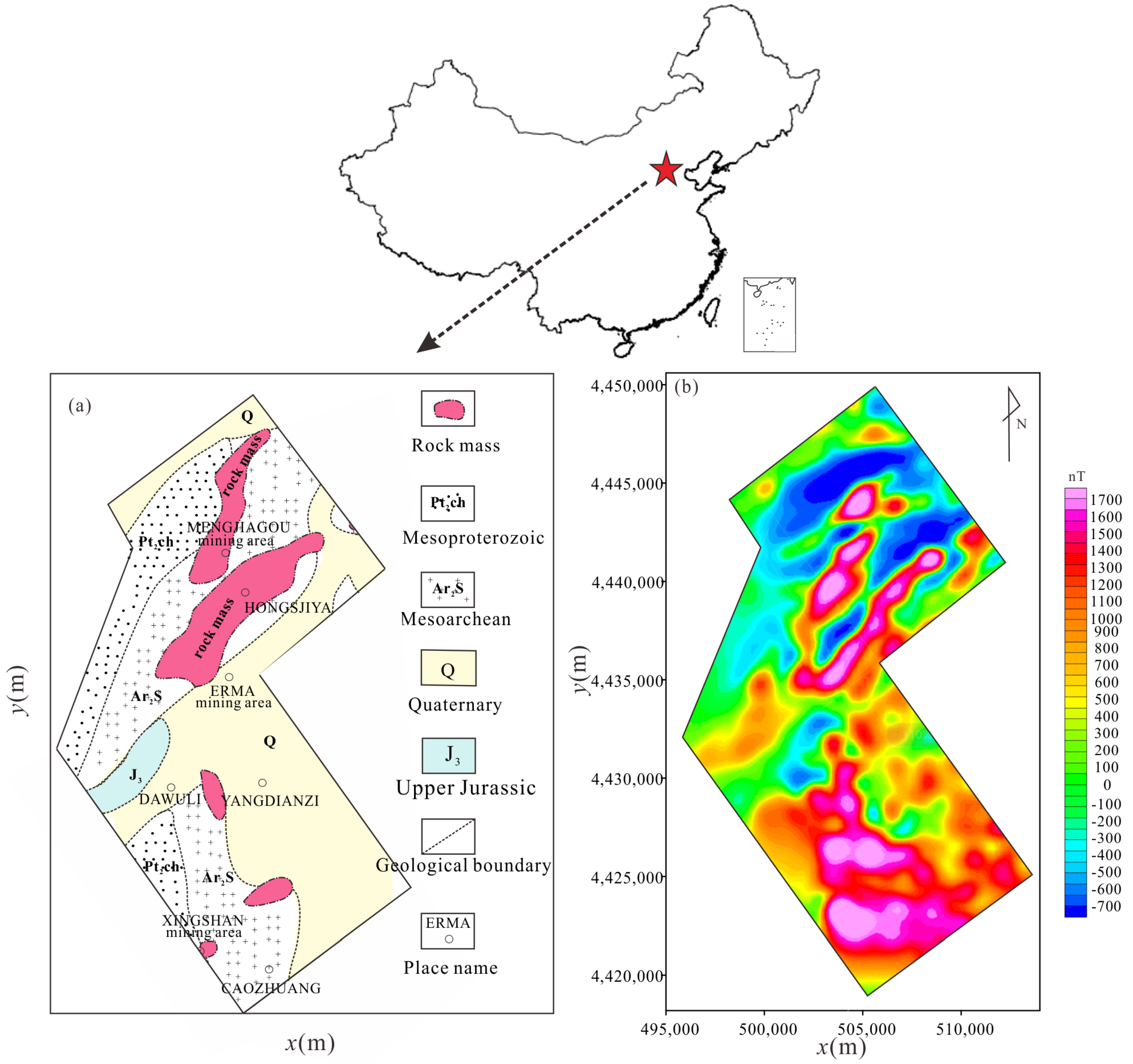
4. Real Magnetic Data Applications

The Qian’an mining area in Hebei province, China, is important for its iron ore production. Figure 8a shows the regional geology map with the iron-bearing rock mass of the geological inferences highlighted in pink. The southern part of the area is a thick covered area of the Quaternary system. It lacks outcrops, and the range of nearby iron ore resources cannot be determined from the geological map.
An aeromagnetic survey was carried out to determine the specific distribution of the iron ore. The mean flight altitude was 80 m, the data sample interval was 50 m, and the flight direction of the survey line was 320°. The aeromagnetic anomaly obtained after vertical and horizontal acceleration correction, as well as posture, Eotvos, zero displacement, base, normal field and Bouguer corrections, is shown in Figure 8b.
We applied the Butterworth filter to the data, prior to applying our method. We saw that the trend of the magnetic anomalies in a northeast direction was similar, but there was a large-scale high-magnetic anomaly in the southern part of the area, implying that there were iron ore resources underground.
We applied different combinations of local wavenumbers to interpret the magnetic data observed in the Qian’an region to locate iron ore deposits. Figure 9a shows the locations of the source estimated by estimator C1. Figure 9b,c show the superimposed results computed by estimators Cd and Bd, respectively, and the results showed less scattering. The depth of the source was concentrated between 150 and 450 m. Figure 9d shows the structural index estimated by estimator Bd. The value at the peaks is close to 1, which is marked by a triangle, indicating that the source was almost a sphere. This might reflect the fact that the flight lines were far apart, so the 2D features that were oblique to the flight lines, and should have formed linear anomalies on the grid, formed a number of discrete anomalies, such as on our map. We have modified the geological map based on the inversion results and revised the locations of the magnetic formations (dark red) in Figure 10. The modified magnetic formations range is similar to geological inference and more detailed in local areas. There were four large magnetic features that were interpreted as iron ore deposits.

5. Discussion and Conclusions

For aeromagnetic data, we proposed a new method of combined local wavenumbers. The combinations of equations that gave the best results (for all parameters which they were being used to estimate) were two combinations that involved two equations with first- and second-order wavenumbers, respectively (estimators Ad and Bd). On synthetic profile data, the original local wavenumber method solved the field source position and the structural index at the same time. On this basis, our method obtained better results than the original local wavenumber method. When the latter two methods were tested with noise-corrupted data, they also gave good results. When there were multiple anomalies on the profile, estimator Ad and Bd also gave good results, but estimator A1 gave inaccurate results. On gridded data only two of the original four equations could be extended to solve for three position parameters (easting, northing and depth), so there was only one possible new combination. This combination (estimator Cd) only yielded the three position parameters; however, the strike direction was determined, and estimator Bd was used on profiles extracted from the grid to estimate the position and structural index. For aeromagnetic data, we obtained results with a low spatial spread of position estimates using estimators Bd and Cd and determined the structural index from estimator Bd. From the resulting images we were able to refine the geological map.

Author Contributions

Conceptualization, G.M. and N.W.; methodology, G.M.; software, G.M. and N.W.; validation, G.M., N.W. and L.L.; formal analysis, N.W.; data curation, N.W.; writing—original draft preparation, N.W.; writing—review and editing, G.M. and L.L.; visualization, G.M.; supervision, G.M.; project administration, N.W.; funding acquisition, L.L. All authors have contributed significantly and have participated sufficiently to take responsibility for this research. All authors have read and agreed to the published version of the manuscript.

Funding

This research was supported by the National Natural Science Foundation of China (42074147).

Informed Consent Statement

Not applicable.

Data Availability Statement

Not applicable.

Acknowledgments

The authors also thank the anonymous reviewers for their constructive comments and suggestions.

Conflicts of Interest

The authors declare that they have no conflict of interest.

Appendix A

The Euler equation for 2D bodies was defined as [10]:
( x x 0 ) f x + ( z z 0 ) f z = N ( f + B )
where B represents the background field.
Taking the derivatives of Equation (A1) in the horizontal and vertical directions, respectively, we obtain:
( x x 0 ) 2 f x 2 + ( z z 0 ) 2 f z x = ( N + 1 ) f x
and:
( x x 0 ) 2 f x z + ( z z 0 ) 2 f z 2 = ( N + 1 ) f z
Then, taking the horizontal derivative of Equations (A2) and (A3), we obtain:
( x x 0 ) 3 f x 3 + ( z z 0 ) 3 f z x 2 = ( N + 2 ) 2 f x 2
and:
( x x 0 ) 3 f x 2 z + ( z z 0 ) 3 f z 2 x = ( N + 2 ) 2 f x z
Multiplying Equation (A4) and Equation (A5) by 2 f x 2 and 2 f x z , respectively, and then adding them, we get:
( x x 0 ) [ 3 f x 3 2 f x 2 + 3 f x 2 z 2 f x z ] + ( z z 0 ) [ 3 f z x 2 2 f x 2 + 3 f z 2 x 2 f x z ] = ( N + 2 ) [ ( 2 f x 2 ) 2 + ( 2 f x Z ) 2 ]
Substitute the Laplace equation into Equation (A6), and we obtain:
( x x 0 ) [ 3 f z 2 x 2 f x 2 3 f x 2 z 2 f x z ] [ ( 2 f x 2 ) 2 + ( 2 f x Z ) 2 ] + ( z z 0 ) [ 3 f z 2 x 2 f x z 3 f z x 2 2 f z 2 ] [ ( 2 f x 2 ) 2 + ( 2 f x Z ) 2 ] = ( N + 2 )
According to the definition of local wavenumber, Equation (A7) can be rewritten as:
k 2 z ( x x 0 ) + k 2 x ( z 0 z ) = N + 2
Multiplying Equations (A4) and (A5) by 2 f x Z ( 2 f x 2 ) 2 + ( 2 f x Z ) 2 and 2 f x 2 ( 2 f x 2 ) 2 + ( 2 f x Z ) 2 , respectively, and then subtracting each other, we get:
( x x 0 ) [ 3 f z 2 x 2 f x z 3 f z x 2 2 f z 2 ] [ ( 2 f x 2 ) 2 + ( 2 f x Z ) 2 ] + ( z z 0 ) [ 3 f z 2 x 2 f x 2 3 f x 2 z 2 f x z ] [ ( 2 f x 2 ) 2 + ( 2 f x Z ) 2 ] = 0
According to the definition of local wavenumber, Equation (A9) can be rewritten as:
k 2 x ( x x 0 ) + k 2 z ( z z 0 ) = 0

Appendix B

The Euler equation for 3D bodies was defined as [10,25]:
( x x 0 ) f x + ( y y 0 ) f y + ( z z 0 ) f z = N ( f + B ) .
Taking the derivatives of Equation (A11) in the x, y and z directions, respectively, we obtain:
( x x 0 ) 2 f x 2 + ( y y 0 ) 2 f y x + ( z z 0 ) 2 f z x = ( N + 1 ) f x ,
( x x 0 ) 2 f x y + ( y y 0 ) 2 f y 2 + ( z z 0 ) 2 f z y = ( N + 1 ) f y
and:
( x x 0 ) 2 f x z + ( y y 0 ) 2 f y z + ( z z 0 ) 2 f z 2 = ( N + 1 ) f z .  
Then, taking the vertical derivative of Equations (A12)–(A14), we obtain:
( x x 0 ) 3 f x 2 z + ( y y 0 ) 3 f x y z + ( z z 0 ) 3 f z 2 x = ( N + 2 ) 2 f x z ,
( x x 0 ) 3 f x y z + ( y y 0 ) 3 f y 2 z + ( z z 0 ) 3 f z 2 y = ( N + 2 ) 2 f y z
and:
( x x 0 ) 3 f z 2 x + ( y y 0 ) 3 f y 2 z + ( z z 0 ) 3 f z 3 = ( N + 2 ) 2 f z 2 .
Multiplying Equations (A15)–(A17) by ( 2 f / z 2 ) ( 2 f / z x ) ( f / h ) ( ( f / h ) 2 + ( 2 f / z 2 ) 2 ) , ( 2 f / z 2 ) ( 2 f / z y ) ( f / h ) ( ( f / h ) 2 + ( 2 f / z 2 ) 2 ) and ( f / h ) ( f / h ) 2 + ( 2 f / z 2 ) 2 , respectively, and then adding each other, we get:
( x x 0 ) ( f h ) 2 3 f x z 2 2 f z 2 ( 2 f x z 3 f x 2 z + 2 f y z 2 f x y z ) ( ( f h ) 2 + ( 2 f z 2 ) 2 ) ( f h ) + ( y y 0 ) ( f h ) 2 3 f y z 2 2 f z 2 ( 2 f x z 3 f x y z + 2 f y z 3 f y 2 z ) ( ( f h ) 2 + ( 2 f z 2 ) 2 ) ( f h ) + ( z z 0 ) ( f h ) 2 3 f z 3 2 f z 2 ( 2 f x z 3 f x z 2 + 2 f y z 3 f y z 2 ) ( ( f h ) 2 + ( 2 f z 2 ) 2 ) ( f h ) = 0 ,
where f h = ( 2 f x z ) 2 + ( 2 f y z ) 2 .
According to the definition of 3D local wavenumbers:
k 2 x = ( f h ) 2 3 f x z 2 2 f z 2 ( 2 f x z 3 f x 2 z + 2 f y z 3 f x y z ) ( ( f h ) 2 + ( 2 f z 2 ) 2 ) ( f h ) ,
k 2 y = ( f h ) 2 3 f y z 2 2 f z 2 ( 2 f x z 3 f x y z + 2 f y z 3 f y 2 z ) ( ( f h ) 2 + ( 2 f z 2 ) 2 ) ( f h ) ,
k 2 z = ( f h ) 2 3 f z 3 2 f z 2 ( 2 f x z 3 f x z 2 + 2 f y z 3 f y z 2 ) ( ( f h ) 2 + ( 2 f z 2 ) 2 ) ( f h ) ,
Equation (A18) can be rewritten as:
k 2 x ( x x 0 ) + k 2 y ( y y 0 ) + k 2 z ( z z 0 ) = 0 .

References

  1. Reford, M.S.; Sumner, J.S. Aeromagnetics. Geophysics 1964, 29, 482–516. [Google Scholar] [CrossRef]
  2. Tezkan, B.; Stoll, J.B.; Bergers, R.; Crofbach, H. Unmanned aircraft system proves itself as a geophysical measuring platform for aeromagnetic surveys. First Break 2011, 29, 103–105. [Google Scholar]
  3. Eppelbaum, L.; Mishne, A. Unmanned Airborne Magnetic and VLF Investigations: Effective Geophysical Methodology for the Near Future. Positioning 2011, 2, 112–133. [Google Scholar] [CrossRef] [Green Version]
  4. Ibrahim, A.; Gemail, K.; Abdelrahman, K.; Al-Otaibi, N.; Ibrahim, E.; Saada, S. Multi-Scale Geophysical Methodologies Applied to Image Archaeological Ruins at Various Depths in Highly Terraneous Sites. Remote Sens. 2021, 13, 2055. [Google Scholar] [CrossRef]
  5. Zhu, X.; Zheng, H.; Lu, M. Lateral variation of aeromagnetic anomaly in South China and its tectonic implications. Int. J. Earth Sci. 2019, 108, 1493–1507. [Google Scholar] [CrossRef]
  6. Gao, X.; Xiong, S.; Yu, C.; Zhang, D.; Wu, C. The Estimation of Magnetite Prospective Resources Based on Aeromagnetic Data: A Case Study of Qihe Area, Shandong Province, China. Remote Sens. 2021, 13, 1216. [Google Scholar] [CrossRef]
  7. Ebele, J.E.; Ofoegbu, C.O.; Nur, A. Interpretation of high-resolution aeromagnetic and radiometric data for delineation of mineral potential zones over Abuja and Environs, North-Central Nigeria. Arab. J. Geosci. 2021, 14, 1947. [Google Scholar] [CrossRef]
  8. Elkhateeb, S.O.; Eldosouky, A.M.; Khalifa, M.O.; Aboalhassan, M. Probability of mineral occurrence in the Southeast of Aswan area, Egypt, from the analysis of aeromagnetic data. Arab. J. Geosci. 2021, 14, 1514. [Google Scholar] [CrossRef]
  9. Werner, S. Interpretation of Magnetic Anomalies at Sheet-Like Bodies. Geophys. Prospect. 1953, 57, 447–459. [Google Scholar]
  10. Thompson, D.T. EULDPH: A new technique for making computer-assisted depth estimates from magnetic data. Geophysics 1982, 47, 31–37. [Google Scholar] [CrossRef]
  11. Nabighian, M.N. The analytic signal of two-dimensional magnetic bodies with polygonal cross-section: Its properties and use for automated anomaly interpretation. Geophysics 1972, 37, 507–517. [Google Scholar] [CrossRef]
  12. Salem, A.; Ravat, D. A combined analytic signal and Euler method (AN-EUL) for automatic interpretation of magnetic data. Geophysics 2003, 68, 1952–1961. [Google Scholar] [CrossRef]
  13. Thurston, J.B.; Brown, R.J. Automated source-edge location with a new variable pass-band horizontal-gradient operator. Geophysics 1994, 59, 546–554. [Google Scholar] [CrossRef]
  14. Salem, A.; Ravat, D.; Smith, R.; Ushijima, K. Interpretation of magnetic data using an enhanced local wavenumber (ELW) method. Geophysics 2005, 70, L7–L12. [Google Scholar] [CrossRef]
  15. Bracewell, R. The Fourier Transform and Its Applications. McGraw Hill Book Co.: New York, NY, USA, 1965; pp. 222–224.
  16. Smith, R.; Thurston, J.B.; Dai, T.; MacLeod, I.N. iSPI TM—the improved source parameter imaging method. Geophys. Prospect. 1998, 46, 141–151. [Google Scholar] [CrossRef]
  17. Smith, R.; Salem, A. Imaging depth, structure, and susceptibility from magnetic data: The advanced source-parameter imaging method. Geophysics 2005, 70, L31–L38. [Google Scholar] [CrossRef]
  18. Keating, P. Improved use of the local wavenumber in potential-field interpretation. Geophysics 2009, 74, L75–L85. [Google Scholar] [CrossRef]
  19. Abbas, M.A.; Fedi, M.; Florio, G. Improving the local wavenumber method by automatic DEXP transformation. J. Appl. Geophys. 2014, 111, 250–255. [Google Scholar] [CrossRef]
  20. Ma, G.-Q.; Ming, Y.-B.; Han, J.-T.; Li, L.-L.; Meng, Q.-F. Fast local wavenumber (FLW) method for the inversion of magnetic source parameters. Appl. Geophys. 2018, 15, 353–360. [Google Scholar] [CrossRef]
  21. Ma, G. Improved Local Wavenumber Methods in the Interpretation of Potential Field Data. Pure Appl. Geophys. Pageoph. 2012, 170, 633–643. [Google Scholar] [CrossRef]
  22. Salem, A.; Williams, S.; Fairhead, D.; Smith, R.; Ravat, D. Interpretation of magnetic data using tilt-angle derivatives. Geophysics 2008, 73, L1–L10. [Google Scholar] [CrossRef]
  23. Reid, A.B.; Ebbing, J.; Webb, S.J. Avoidable Euler Errors—The use and abuse of Euler deconvolution applied to potential fields. Geophys. Prospect. 2014, 62, 1162–1168. [Google Scholar] [CrossRef]
  24. Juan, H.H.; Kevin, L.M. Hilbert transform of gravity gradient profiles: Special cases of the general gravity-gradient tensor in the Fourier transform domain. Geophysics 2002, 67, 766–769. [Google Scholar]
  25. Reid, A.B.; Allsop, J.M.; Granser, H.; Millett, A.J.; Somerton, I.W. Magnetic interpretation in three dimensions using Euler deconvolution. Geophysics 1990, 55, 80–91. [Google Scholar] [CrossRef] [Green Version]
Figure 1. (a) Total magnetic anomaly of two cylinders with a magnetic inclination of 60° and a declination perpendicular to strike; (b) first- and second-order local wavenumbers of the magnetic anomaly in Figure 1a; (c) source location results generated by estimator A1 without screening; (d) source location results generated by estimator B1 without screening; (e) source location results generated by estimator Ad without screening; (f) source location results generated by estimator Bd without screening.
Remotesensing 14 00591 g001
Figure 2. (a) Source location results generated by estimator A1 after screening; (b) source location results generated by estimator B1; (c) structural index results generated by estimator B1; (d) source location results generated by estimator A2; (e) source location results generated by estimator B2; (f) structural index results generated by estimator B2; (g) source location results generated by estimator Ad; (h) source location results generated by estimator Bd; (i) structural index results generated by estimator Bd; (j) source location results generated by estimator Dd; (k) structural index results generated by estimator Dd; (l) source location results generated by estimator As; (m) structural index results generated by estimator As; (n) source location results generated by estimator Bs; (o) structural index results generated by estimator Bs.
Remotesensing 14 00591 g002
Figure 3. (a) Total magnetic anomaly of two cylinders with horizontal coordinates (x0) of 40 m and 70 m; (b) source location results generated by estimator A1, using the magnetic anomaly in Figure 3a; (c) source location results generated by estimator Bd, using the magnetic anomaly in Figure 3a; (d) total magnetic anomaly of two cylinders with horizontal coordinates (x0) of 45 m and 65 m; (e) source location results generated by estimator A1, using the magnetic anomaly in Figure 3d; (f) source location results generated by estimator Bd, using the magnetic anomaly in Figure 3d.
Remotesensing 14 00591 g003
Figure 4. (a) Total magnetic anomaly of two infinite vertical sheets having a magnetic inclination of 60° and a declination perpendicular to strike; (b) source location results generated by first-order Euler deconvolution; (c) source location results generated by second-order Euler deconvolution; (d) source location results generated by estimator A1; (e) source location results generated by estimator A2; (f) source location results generated by estimator Ad; (g) source location results generated by estimator B1; (h) source location results generated by estimator B2; (i) source location results generated by estimator Bd.
Remotesensing 14 00591 g004
Figure 5. (a) Total magnetic anomaly of two infinite vertical sheets having a magnetic inclination of 60° and a declination perpendicular to strike, a noise-corrupted magnetic anomaly with a Gaussian noise of 1% and a noise-corrupted magnetic anomaly with a subsequent Gaussian filter; (b) source location results generated by first-order Euler deconvolution method after filtering; (c) source location results generated by second-order Euler deconvolution method after filtering; (d) source location results generated by estimator A1 after filtering; (e) source location results generated by estimator A2 after filtering; (f) source location results generated by estimator Ad after filtering; (g) total magnetic anomaly of two infinite vertical sheets having a magnetic inclination of 60° and a declination perpendicular to strike, noise-corrupted magnetic anomaly with a Gaussian noise of 3% and noise-corrupted magnetic anomaly with a subsequent Gaussian filter; (h) source location results generated by Euler deconvolution method after filtering; (i) source location results generated by Euler deconvolution method after filtering; (j) source location results generated by estimator A1 after filtering; (k) source location results generated by estimator A2 after filtering; (l) source location results generated by estimator Ad after filtering; (m) RMS between the true depths and average of all the depths computed by estimators A1, A2 and Ad with decreasing noise.
Remotesensing 14 00591 g005
Figure 6. (a) Magnetic anomaly of four cylinders having a magnetization inclined at 60°; (b) first- and second-order local wavenumbers of magnetic anomaly in Figure 5a; (c) source location results generated by estimator A1; (d) source location results generated by estimator Ad; (e) source location results generated by estimator Bd; (f) structural index results generated by estimator Bd; (g) source location results generated by estimator Dd; (h) structural index results generated by estimator Dd.
Remotesensing 14 00591 g006
Figure 7. (a) The total field anomaly of two geological bodies having a magnetization inclined at 60°; (b) source location results generated by estimator C1; (c) source location results generated by estimator C1 in y direction view; (d) source location results generated by estimator Cd; (e) source location results generated by estimator Cd in y direction view; (f) source location results generated by estimator Bd; (g) source location results generated by estimator Bd in y direction view; (h) statistics of structural index estimates generated by estimator Bd.
Remotesensing 14 00591 g007
Figure 8. (a) Regional geology map of survey area; (b) measured magnetic anomaly.
Remotesensing 14 00591 g008
Figure 9. (a) Source location obtained by estimator C1; (b) source locations obtained by estimator Cd; (c) source locations obtained by estimator Bd; (d) structural index obtained by estimator Bd.
Remotesensing 14 00591 g009
Figure 10. Revised or modified magnetic features (dark red), compared with the geological inferences (pink).
Remotesensing 14 00591 g010
Publisher’s Note: MDPI stays neutral with regard to jurisdictional claims in published maps and institutional affiliations.

