Abstract
Estimates of migratory waterbirds population provide the essential scientific basis to guide the conservation of coastal wetlands, which are heavily modified and threatened by economic development. New equipment and technology have been increasingly introduced in protected areas to expand the monitoring efforts, among which video surveillance and other unmanned devices are widely used in coastal wetlands. However, the massive amount of video records brings the dual challenge of storage and analysis. Manual analysis methods are time-consuming and error-prone, representing a significant bottleneck to rapid data processing and dissemination and application of results. Recently, video processing with deep learning has emerged as a solution, but its ability to accurately identify and count waterbirds across habitat types (e.g., mudflat, saltmarsh, and open water) is untested in coastal environments. In this study, we developed a two-step automatic waterbird monitoring framework. The first step involves automatic video segmentation, selection, processing, and mosaicking video footages into panorama images covering the entire monitoring area, which are subjected to the second step of counting and density estimation using a depth density estimation network (DDE). We tested the effectiveness and performance of the framework in Tiaozini, Jiangsu Province, China, which is a restored wetland, providing key high-tide roosting ground for migratory waterbirds in the East Asian–Australasian flyway. The results showed that our approach achieved an accuracy of 85.59%, outperforming many other popular deep learning algorithms. Furthermore, the standard error of our model was very small (se = 0.0004), suggesting the high stability of the method. The framework is computing effective—it takes about one minute to process a theme covering the entire site using a high-performance desktop computer. These results demonstrate that our framework can extract ecologically meaningful data and information from video surveillance footages accurately to assist biodiversity monitoring, fulfilling the gap in the efficient use of existing monitoring equipment deployed in protected areas.
1. Introduction
Sound wildlife and habitat conservation policies and effective practices depend on timely and reliable species monitoring data [1,2,3]. Species monitoring has become one of the critical responsibilities of conservation personnel in protected areas [4,5]. The traditional ground survey is an essential means of species monitoring. However, it is time-consuming, laborious, and difficult to standardize [6,7], potentially leading to biased datasets [8]. In recent years, emerging technologies, such as airborne and spaceborne imagery, biotelemetry, real-time static and video surveillance, and passive acoustic recording [9], have drastically increased data collection capacity with improved efficiency [10] and accuracy [11,12] by reducing operational costs and expanding coverage relative to conventional methods, thereby offering new opportunities for conservation studies at local, regional, and global scales. Ecology and conservation are now in the era of big data [13,14].
Real-time video surveillance devices have many advantages in assisting species surveys such as remote and nonintrusive observation, real-time monitoring, cloud storage, and playback convenience [15,16]. High-definition monitoring equipment installed in protected areas provides many conveniences and advantages for discovering new species, monitoring the behavior of specific species, investigating the home range of animals and their habitat use patterns [17,18], preventing illegal trading, and promoting public awareness [19]. In the past decade, to reduce the cost, labor, and logistics of observations, more managers of protected areas around the world are installing high-definition video surveillance equipment to assist in the daily management of protected areas [20,21]. Video surveillance is particularly useful for wetland ecosystems, where access is often restricted.
The essence of video data is a massive volume (e.g., in terabytes and petabytes) of time-series images [22]. While the increasing amount of data allows unprecedented insights on conservation biology and ecology [14], it also brings the dual challenges of storage and analysis [23], and there is currently a mismatch between the ever-growing volume of raw materials (e.g., video and audio records, images) and our ability to process, analyze, and interpret data to inform conservation [24], which could lead to the loss of a large amount of data [25]. Central challenges for data analysis are large data volume and high data heterogeneity (e.g., multisources, and variable quality and uncertainty), which precludes the traditional likelihood-based modeling approaches due to high computation demands [23] Machine learning (ML), a likelihood-free approach, can automatically generate predictive models by detecting and extracting patterns in data without presumptions concerning structure data [24]. In the past two decades, various machine learning approaches (e.g., ANN—artificial neural networks, RF—random forest, and SVM—support vector machine) have been applied in ecology and conservation for studies such as clustering and classification [25]. Deep learning (DL) or deep neural network (DNN), a family of ML models involving ANN with multiple hidden layers [26], has emerged as a promising approach to link big data and conservation and ecology [25], and became the preferred solution for automated image-based (e.g., video) and signal-based (e.g., audio) data analysis [26,27]. Researchers are now beginning to apply DL to automatically extract scalable ecological insights from complex nonlinear data such as noisy videos and acoustic data [28]. Examples include automated species identification (reviewed by [29]), animal behavior ecology [30], environmental monitoring and ecological modeling [25], genomics [31], and phylogenetics.
Many migratory waterbirds in the East Asian–Australasian flyway (EAAF), a region with 37 countries stretching from Russian Tundra to the coasts of Australia and New Zealand, are a global conservation priority because anthropogenic pressures, such as loss and degradation of habitats, interruption of migratory routes, overexploitation, and global climate change, have threatened their continuing existence [32,33,34]. Therefore, monitoring the wader populations at significant sites within EAAF is an urgent task for establishing and evaluating conservation policies and actions [35,36]. However, in addition to weak contrast with the background, varied body size, and clustering distribution [37], the transient nature of migration at these sites poses a great challenge for accurate estimation of the waterbird abundance and distribution using a particular site with traditional point counts or line transects. Surveys based upon a “snapshot” of waterbird abundance could potentially bring bias in population estimations. Given the successful applications of DL in crowd density estimation using surveillance video [38], and the rapid development of DL theory for processing infrared camera, aerial, and satellite images [39,40,41], this study aims to evaluate the potential of DL in monitoring the abundance and distribution of migratory waterbirds. Taking advantage of the large volumes of accumulated surveillance video data from a recently constructed roosting site, we developed a two-step automatic waterbird monitoring framework for generating high-frequency waterbird density maps to unlock the potential of DL in migratory waterbird monitoring. Our approach could contribute to the modernization of collecting wildlife abundance and distribution data by connecting ecologists and computing scientists.
2. Materials and Methods
2.1. Study Site
We conducted this study on a 50 ha restored site, named “TZN720” within the Tiaozini coastal wetland in Dongtai City, Jiangsu Province, China (Figure 1a,b). TZN720 was an aquaculture pond before 2019 but was converted to wetland managed specifically as high-tide roosting habitat for migratory waterbirds. Tiaozini coastal wetland has a total area of about 333 km2, consists of mainly intertidal wetlands and aquaculture ponds (Figure 1b). The Tiaozini coastal wetland area is inscribed in the World Heritage List as part of the migratory bird sanctuaries along the Yellow Sea–Bohai Gulf of China. The wetland system is an irreplaceable and indispensable hub for over 400 bird species and critical for the over 50 million migratory birds moving along the East Asian–Australasian flyway [42], including the critically endangered spoon-billed sandpiper (Calidris pygmaea), endangered spotted greenshank (Tringa guttifer), and black-faced spoonbill (Platalea minor) [43,44].
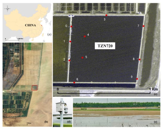
Figure 1.
Overview of the Tiaozini wetland. The red point in (a) is a key staging site for migratory waterbirds, located in the east coast of Dongtai City, Jiangsu Province, China. The study site TZN720, the red square in (b), is a restored wetland and the monitoring site within the Tiaozini wetland; the red dots in (c) show the location of the 10 surveillance cameras; (d) shows the setup of a surveillance camera; and (e) is a panoramic view of TZN720 obtained from the cameras.
Along the elevation gradient, TZN720 has four types of habitat with different microtopography: low levee bank, shallow grass area, shallow water area, and deep water area (Figure 1e). The water level has been kept mostly constant with occasional water exchange with the sea during high tide. The nearest distance from the site to the intertidal zone, where the waterbirds feed, is less than 0.3 km, and the longest distance is no more than 0.9 km, providing an ideal roosting area for waterbirds during high tide [45].
Ten billiard video surveillance cameras from Dahua (DH-SD-49D412U-HN, Zhejiang, China) were installed at TZN720 (Figure 1c) in 2021 and have been monitoring the site since, accumulating extensive video footage. The ONVIF (Open Network Video Interface Forum) cameras are visible and accessible via IP addresses. Each camera is fixed at 1.70 m from the ground and has a maximum zoom range of 60 times, enabling clear bird images. The camera can be rotated 360° horizontally and from −45° to 90° vertically. It can also operate from −40° to 40° Celsius or in an environment with up to 93% humidity.
2.2. Build a Bird Population Counting Dataset
As shown in Figure 2, in order to carry out neural network training, we need to make a bird population counting dataset. The dataset will be introduced from the following three processes: data collection, filtering, and annotation.
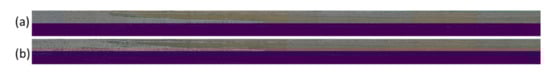
Figure 2.
Samples of the dataset. We show two samples (a,b) from the dataset, where each sample consists of the original image (upper) and the ground truth (lower).
2.2.1. Dataset Collection
PyCharm 3.2.2021 [46], an integrated development environment for Python, was used to call the video track from randomly setup tours to obtain a video that contains information about the entire scene. We used OpenCV [47] to obtain the keyframes, which were named according to the number. The length of video captured in one panorama is four seconds, and each second is composed of thirty frames of images, a total of 120 images. After the test, key image frames of fixed sequence (19, 26, 33, 41, 49, 56, 63, 71, 79, 86, 92, 99, 106, 110, 116) were extracted from the video. Finally, we mosaicked the keyframes in matrix order with the photos captured from the video stream to obtain a panoramic photo of the entire site.
The data feature complexity is high because of the highly frequent interhabitat movements of birds and the change of weather as well. Therefore, to obtain a dataset suitable for neural network training, it is necessary to filter the camera’s large amount of data. To obtain data sets of different scenes and scales, the camera’s focal length, angle, and shooting scene were diversified when collecting data. To obtain a variety of data sets, we randomly sampled these ten cameras to ensure the diversity of the panorama image datasets we obtained (Figure 1c) between 1 June and 9 August.
2.2.2. Data Filtering
To make a dataset for neural network training, it is necessary to filter the camera’s large amount of data. To improve the quality of the dataset, we selected samples with high image quality from all datasets to form the final data set, which is mainly based on the following three steps:
- A.
- Image resolution: Because the image features are not apparent, the image mosaic is incomplete, and some data are lost, so the images with a resolution lower than 4k in the dataset are removed.
- B.
- Image sharpness: Since the images collected by the camera in the rotation process are affected by motion blur, it is necessary to remove the samples with unclear photos in the data set.
- C.
- Data statistical characteristics: To ensure the rationality of data set distribution and the effectiveness of neural network training, it is necessary to reasonably allocate the number of samples with different number scales in the data set. We removed the pictures with less than 10 targets in the dataset and screened the images with a larger number of scales (ranging from 50 to 20,000) to ensure a reasonable distribution of the dataset.
2.2.3. Data Annotation
We developed an annotation tool for bird population counting. As shown in Figure 3, a point was placed at the center position of a target and the coordinates of the point were saved, representing a bird. Panoramic images are generally long. However, desktop computers have limited display size, and it is difficult to directly annotate panorama images using a desktop computer. Therefore, we preprocessed all samples in the data set to improve the labeling efficiency and reduce the labeling cost. The preprocessing procedure is divided into three steps.
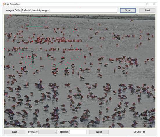
Figure 3.
The interface of the annotation tool. Every bird in an image is marked as a red dot, and the coordinated points are saved for further counting.
- A.
- Determining the minimum unit of image clipping: The input size of the density estimation module designed in this method is fixed at 1024 × 768, which can ensure the computational efficiency of the algorithm and retain the valuable feature information of the image as much as possible.
- B.
- Resizing the original image: The size of the original image is not regular. The length range is 4k~30k, and the width is 1k~1.2k. It cannot be cut into multiple 1024 × 768 images. Therefore, it is necessary to resize the original image and round it to a multiple of 1024 × 768.
- C.
- Clipping the resized image: After three steps of clipping preprocessing, the original dataset is clipped into many small images of 1024 × 768, which improves the labeling efficiency, and the labeled label information can be mapped to the original data through the corresponding relationship between file name and image size.
2.3. Build a Panorama Bird Population Counting Network
As shown in Figure 4, the network’s input is a panoramic “RGB“ image, and the output is a density map showing the bird distribution within the monitoring area. The process of network construction consists of three steps.
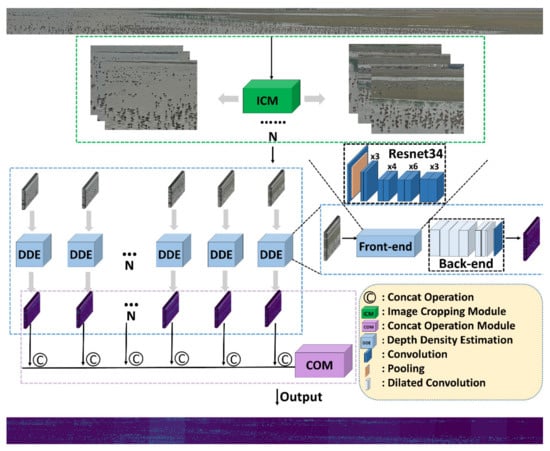
Figure 4.
The architecture of panorama bird population counting network. It consists of three parts, the green part is the image cropping module, the blue part is the depth density estimation network, and the purple part is the concat operation module.
First, the input image is automatically cropped into n pending images with the size of 1024 × 768 through the image clipping module. Second, the depth density estimation network (DDE) estimates the bird density of the clipped images. Third, the concat operation module (COM) splices the generated density images into a panoramic bird density map for the entire site and calculates the total bird abundance.
2.3.1. Image Clipping Module
Due to the uncertainty of rotation parameters of image acquisition equipment, the size of image data obtained is not fixed. Therefore, we first scale the size of the image so that the pixel length of the picture is the integer multiplication 1024 and the pixel width of the picture is the integer multiplication 768, and then the image is cut into clips with the same size, 1024 × 768. We designed an automatic clipping method to obtain N minimum processing image units. The formula follows:
where N is the minimum number of processing units x after cropping, y is the real pixel value of the input image, is a fixed length of 1024 pixels, is a height of 768 pixels. Input images of actual pixel values are divided by 1024 (number of fixed pixel values); the whole integer input image of actual pixel values is divided by 1024 (number of static pixel values), recorded, and replaced with the entire integer b. The actual pixel value of the input image m is divided by 1024, which results in the fixed pixel value remainder λ. This is used to adjust the size of the y-direction proportion.
2.3.2. Depth Density Estimation Network
Many waterbirds are small and congregate into flocks during foraging and roosting [48]. To determine the number of flocks in a given image, we first generate a density map based on the experience gained from crowd counting. Relative to the total number of birds, the density map can show the spatial distribution of birds in a given image. We use an adaptive Gaussian blur algorithm to generate density map labels. The process mainly includes two parts: image annotation display and image conversion and representation. First, a two-dimensional matrix with the exact resolution as the original image is generated. Then the coordinates are transformed by the input and output resolution ratio. The transformed label coordinate xi is then set to 1 by the delta function, which is given as:
Next, we convolve the two-dimensional Gaussian kernel with the delta function. However, the of the different samples are not completely independent; they are related to each other due to perspective distortion. Therefore, we must consider the problem of perspective deformation when dealing with it. Using the K-nearest neighbor algorithm, we calculate the current sample point and the surrounding sample point in
where is the average distance corresponding to each sample, and β is a scaling parameter. Through experimentation, we found that the best result is obtained when β = 0.5.
We propose a neural network model called depth density estimation (DDE) network for bird density estimation. The DDE model comprises two parts: the front-end feature extraction and the back-end density map generation. As the background of the image data is complex, containing information about various objects, we choose to use the deep residual network with the best effect in the field of image recognition for front-end feature extraction [49]. The bottomless residual network extends the deep neural network to 152 layers by employing short-circuit connection. It effectively improves the extraction of image features by neural network and solves the problems of degradation and difficulty in training and convergence with the deepening of the neural network [49]. The ResNet network is modified based on the VGG network [50], and the residual unit is added through the short-circuit mechanism, which alleviates the problem that the deep network is difficult to train. It has five structures with different depths, among which the ResNet152 deepens the network structure based on ResNet34 and has stronger feature extraction ability. Considering both the accuracy of the whole network and the execution efficiency of the algorithm, we abandoned ResNet152 with the highest accuracy. We chose the ResNet34 network with high computing speed under the premise of losing a small amount of accuracy as the front-end feature extraction part to connect with the back-end density map generation part. We removed ResNet’s entire connection layer. In addition, ResNet34 is pre-trained on ImageNet [51], a ten-million-level dataset, and the weight contains rich target feature information. Therefore, using this network structure as a feature extraction network can effectively accelerate the convergence speed of network training.
Dilated convolution increases the receptive field of convolution operation by adding a hole calculation operation to the convolution core to make the output of each convolution contain an extensive range of information without a pooling operation. In the ordinary convolution operation, the size of the convolution core is 3 × 3, and its receptive field is 3 × 3. In the dilated convolution with dilation 1, although the extent of the convolution core is 3 × 3, the receptive field becomes 7 × 7. The birds in the dataset are small and individual occlusion is expected; thus, we need more abundant and complete local feature information to generate the feature map. Therefore, we choose hole convolution as the main component of the back-end density map generation part. To retain the image feature information as much as possible, we do not use the pooling layer.
The labeling is a crucial step in neural network training [52]. The reliability of data labels directly determines the accuracy of supervised learning results. When generating the dataset label, the dataset uses the label from the population density estimation dataset for reference. Because ResNet34 uses multiple dimensionality reduction operations in developing the density map, the size of the density map is 1024 times the size of the original image; it is therefore necessary to resize the label data. After experimentation, it was found that after using the resize operation directly, the label difference generates an error, and the error calculation formula is:
where M is the number of samples in the dataset, (m, n) are the coordinates of image pixel points, and is the number of birds read directly from the label file.
As shown in Table 1, when the number of downsampling times exceeds four, the label produces errors that dramatically affect the algorithm’s accuracy. Although the error is relatively small if the downsampling is less than four times, the number data to be processed by the algorithm increases with the increase of the output characteristic graph, and the algorithm is not suitable for convergence. Therefore, two-dimensionality reduction operations are removed from DDE. The size of the output feature graph is 128 × 96, which not only ensures the convergence speed of the algorithm, but also ensures the algorithm’s accuracy.

Table 1.
Density map label error with different downsampling operations.
2.4. Model Training
We applied the DDE model to the dataset collected from TZN720 to estimate the abundance of birds staging in this world heritage site. We randomly set 80% of the images for model training and the remaining 20% for model testing and validation.
DDE was developed using PyTorch 1.8.0. The model is trained in Geforce RTX3090 with 24 GB memory. The initial model specifications were set as follows: learning rate = 10 × 10−5, batch size = 1, momentum = 0.95, weight attenuation = 5 × 10 × 10−4, and 200 epoch for the iteration cycle. It took 18 h to train the model.
2.5. Performance Evaluation
In order to verify the effectiveness of our approach, we calculated the mean absolute error (MAE) and the root mean square error (RMSE) of our algorithm:
where N is the number of images to be tested, Zi is the ground truth (manually labeled by 20 workers, representing the real bird counts in the picture) of the ith image, which is the model prediction.
While MAE gives an indication of the algorithm’s accuracy, MSE assesses the algorithm’s robustness and stability. To further express the accuracy of the algorithm directly, we calculated the accuracy of the algorithm defined as:
The lower MAE and , the greater the accuracy of the algorithm in the test set, and the lower MSE, the more stable and better adaptability of the algorithm. In addition, we calculated the model MEA, RMSE, and accuracy with a different sample size of the testing dataset to illustrate the effectiveness of our method.
To our best knowledge, there is currently no neural network algorithm specifically applied to bird density estimation, so we compared the performance of our algorithm with six popular crowd density estimation algorithms. We trained the six algorithms (i.e., MCNN [53], MSCNN [54], ECAN [55], MSPNet [56], SANet [57], and CSRNet [58]) with our bird dataset using the transfer learning method basis on original weights, and compared s.
2.6. Motivating Application: Exploring Daily Movement of Waterbirds by Using High-Frequency Population Counting
Tidal height is an important factor affecting the habitat of waterbirds in coastal ecosystems [59] and tidal cycle drives the between-habitat movement and foraging behavior of waterbirds [60]. In order to explore the relationship between bird abundance at roosting sites and tidal height, we used camera 3 (Figure 1c) to monitor areas with a high concentration of waterbirds. Between 9 August and 1 October, it is still the peak mitigation season, and there were a large number of waterbirds that migrated into the Tiaozini coastal area. We selected 13 days during this period when the high tides could completely submerge the mudflats—the foraging ground of waterbirds. For each of these 13 days, we generated a panorama image from 6:00–18:00 at intervals of 5 min. We collected 984 panoramic images of key habitats in TZN720 and ultimately applied the trained model to estimate the number of roosting birds.
We also collected the tide data for the same period from the China Maritime Safety Administration [61]. We used the Lagrangian interpolation method implemented in Pycharm (3.3) to fill the gaps in the raw tide data, resulting in a regular time series of tidal height with an interval of 5 min. For illustrating the relationship between waterbird abundance and tidal height, R version 4.1.2 was used with the following packages: cowplot_0.9.4 [62], ggplot2_3.1.0 [63], and RColorBrewer_1.1-2 [64].
3. Results
3.1. The Panoramic Bird Population Counting Dataset
The whole dataset covers different camera scenes and has rich feature information. The dataset contains a total of 935 panoramic images of different sizes (Figure 5). It took 20 people three months to label and count the birds in these images. Manual counting revealed that there are 787,552 birds in this dataset. The number of birds captured by these images varied dramatically (mean = the average picture includes 842.30 and SD = 2089, Figure 6).
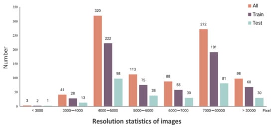
Figure 5.
The distribution of image resolution and corresponding image quantity in the bird dataset.
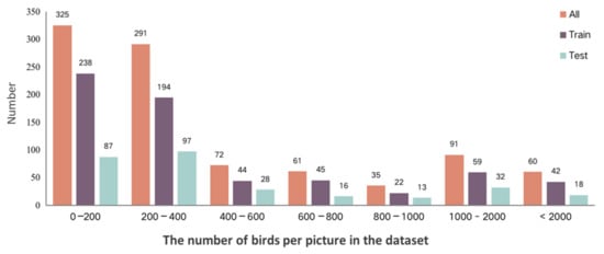
Figure 6.
The distribution of the number of birds and the corresponding number of training and testing images.
3.2. Model Performance
The MAE and RMSE of the image processing algorithm are 120.86 and 599.74, respectively. Meanwhile, the average error rate is 14.14%. The image processing rate is 2.12 FPS (frames per second). The average recognition accuracy of the image was 85.59% (SD = 0.1273, SE = 0.0004). Although it varied with the number of targets in the image, the average accuracy of the model was comparable for mapping and counting up to 2000 targets per image, and peaked at 90.92% (SD = 0.0788) when the number of birds in the image was 800–1000 (Figure 7). The accuracy deteriorated when the number of birds in the image was greater than 2000 (mean = 78.63% and SD = 0.1382, Figure 7).
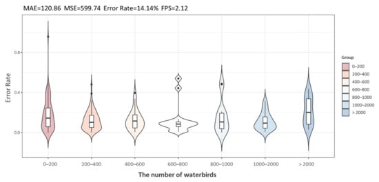
Figure 7.
Distribution of absolute error rates in each group. The x-axis represents a grouping of panoramic images of different bird populations of magnitude. The number of birds contained in the panoramic image has different effects on the accuracy of the model.
Example of model products, including density map and total bird count, are presented in Figure 8. It is clear that our method has good adaptability to scenes with different sizes, distinct target density, and congregation patterns.
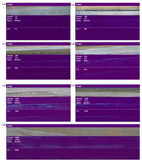
Figure 8.
Examples of model output of density map and bird counting. We visualize the results of different orders of magnitude images to demonstrate the adaptability and practicability of our algorithm: (a–g) represent seven typical samples of different orders of magnitude, each consisting of the original image (top) and the resultant density map (middle) and total bird count in the image (bottom).
3.3. Comparison with Other Deep Learning Algorithms
In comparison with other neural network algorithms that were applied in crowd density estimation, our approach had the lowest MAE of 120.86 and lowest RMSE of 599.74 (Table 2), obviously outperforming the others. Other algorithms have better results in estimating population density in other studies, but the accuracy decreases when estimating waterbird populations in this study. Moreover, in terms of computing cost, our approach was also among the algorithms with high efficiency (Table 2).
Table 2.
Comparison with other algorithms: we compared the current mainstream crowd density estimation algorithms, and our algorithm has the highest accuracy.
3.4. Tidal-Driven Waterbird Movement in Tiaozini
The relationship between the number of roosting waterbirds and tidal height is presented in Figure 8. The estimated number of roosting waterbirds traced the tide dynamics closely; as the tide rose, so did the number of roosting waterbirds (Figure 9a). However, the rate of change of the roosting waterbirds at falling tide was dramatically faster than at rising tide. The birds gathered slowly at rising tide, which suggested that the waterbirds foraging between tides were likely to linger in the intertidal zone for a longer period of time. When the tide receded and the mudflats were exposed, the birds tended to leave the roosting site quickly (Figure 9b). It is worth noting that it takes about 2.5 h to count 75 percent of the birds in this site during a field survey.
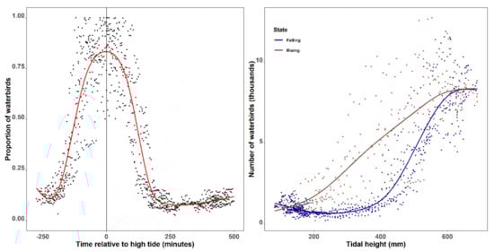
Figure 9.
The relationship between waterbird abundance at the roosting site and tide height based on estimations from 984 images extracted from surveillance video data collected for the peak autumn migratory season (9 August and 1 October). Dots are estimated abundance dashed and lines are gam smoothed curve. Left panel shows the variation of waterbird abundance (percentage to the total count) at the roosting site during a tidal cycle. Right panel illustrates the relationship of the number of waterbirds at the roosting site and tidal heights during periods of rising (dark brown) and falling (dark blue) tide.
4. Discussion
4.1. Overall Accuracy and Innovation
Many previous studies have demonstrated the high performance of using DL for animal recognition and detection from surveillance videos and estimate wildlife abundance from static images such as aerial photos and pictures from citizen science smartphone applications [65,66,67,68]. Few studies have documented the efficiency of DL for quantifying animals from real-time surveillance video [69] despite the recent development on crowd density estimation (see references in Table 2). By combining video streaming and DL animal recognition and counting, our proposed framework achieved good accuracy with an overall error rate of 14.14%. In addition, the DDE module with ResNet34 performed consistently well for images with diversified bird density and congregation patterns, and the accuracy for images containing more than 2000 individual birds was 78.63%. This is acceptable for conservation. These results demonstrate that our approach can realize the full potential of computer vision for wildlife monitoring and conservation [70].
Previous applications of DL for automatic image processing tend to be of low resolution [71]. In our study, the image resolution of the data set is more than 4k, and some even more than 30k. This fine resolution has higher requirements for computing equipment, which requires Intel(R) Core (TM) i7-8700 CPU and GPU 2080ti or higher. Moreover, with an increase in image resolution, the model’s ability to extract local information decreases. We resolved this problem by clipping the large images, which improved the model’s training and reasoning ability and the model’s attention to the local spatial information of the original picture.
Once the model was trained, it was efficient to predict the number of waterbirds presented in an image and produce a density map (average processing rate was 2.12 FPS), enabling high-frequency abundance estimates. Using the model, we successfully regenerated the waterbird movement within a stopover site during a tidal cycle by using 984 images extracted from surveillance video data. Our results have a clear implication for the data collection methodology for protected areas as well as for conservation efforts of EAAF, where monitoring population trends with standardized and coordinated methods are a priority [36]. Our approach also provides local managers with an automatic system that can report any change in the behavior of birds that warrants urgent attention, particularly in remote and underfunded areas where regular patrolling is impossible.
4.2. Limitations and Prospects
Many factors, including pixel size of the monitoring target, the complexity of background information, the accuracy of the label, and the picture quality of the original image, affect the accuracy of the model for crowd counting and density mapping [72,73], and, in particular, the correctness of the label information. This algorithm is a neural network algorithm based on supervised learning, which needs to continuously optimize the parameters of the algorithm by providing the correct label information corresponding to the samples for the algorithm. Therefore, the accuracy of sample tag information is directly related to the accuracy of the algorithm. To ensure that the trained model has comparable prediction accuracy for real-world scenarios, our training dataset contained images of poor quality, such as images recorded in rainy, foggy, low-light, and bright-light conditions, which could affect the performance of the entire model. It is necessary to investigate how these factors affect prediction power.
Generally, for single image crowd counting, the more targets in an image recognition unit, the higher the stacking level, and the better the recognition. Previous studies on crowd density estimation have shown that DL approaches are more suitable for scenarios with simpler backgrounds with a larger number of targets, which are stacked on top of each other [74,75]. To estimate the abundance of birds using the constructed wetland at a given time, the input panoramic images, which capture the entire view of the scene, were created by mosaicking video frames. Thus, there are areas (e.g., deep waters) with very few targets due to the clustering distribution of waterbirds in stopover sites [48], which could affect the count accuracy of the entire panoramic photo. This may also result in less precision for more extended panoramic images with more birds (Figure 7). Developing approaches that are capable of handling imbalanced (in terms of a number of targets in a scene) training datasets could improve the performance.
Similar to other neural network techniques, training the DL model requires a large amount of training data (i.e., labeled data) to achieve the model’s generalization [10,48,74,75]. However, creating a training data set can be costly and time-consuming. In this study, it required 60 person-months to create the training dataset of 935 panoramic images. Data augmentation, such as image distortion (e.g., shifting, blurring, mirroring, rotation, nearest neighbor pixel swapping) [76] and transfer learning [77], could potentially reduce the cost of collecting training data.
In this study, we treated migratory waterbirds as a group and did not distinguish species. There are situations, such as determining the conservation status of a species, where distribution and abundance data of the targeted species are required. In addition, waterbirds may differ in habitat requirement [59,78] and therefore need different conservation actions. Future research could test the performance of other DL methods, such as target detection, to distinguish and count different species in panoramic images [79]. In the future, mesh sampling methods [6] could also be designed using surveillance cameras already available in reserve to assist in waterbird surveys and to help understand the differences in habitat selection for different waterbirds in different regions.
5. Conclusions
Estimating wild animal abundance is a central task for ecologists and conservationists and the accuracy of the estimations is fundamental to answering many ecological and conservation questions for sound conservation efforts [80]. However, monitoring species abundance can be costly, time-consuming, and logistically difficult as the occurrence of animals and their behaviors often vary over broad spatial and temporal scales [8]. The accurate estimation of the number of migratory waterbirds using a particular stopover site is particularly challenging due to its transient nature. With the large and ever-increasing volume of static and video surveillance data, there is a great potential for collaboration between ecologists and conservationists, and experts in the fields of remote sensing and computer science to generate scalable ecological knowledge for biodiversity and habitat conservation. Recent developments in the field of computer vision and DL have given rise to reliable tools and software of feature extraction for animal recognition, accurate estimation of populations, understanding animal behavior, and habitat use. In this study, we developed a two-step automated waterbird monitoring framework. The first step of image streamlining automatically segments, selects, and mosaics surveillance video into panoramic images covering the entire monitoring area, which is subjected to the second step of bird recognition and annotation, and counting and density estimation using a deep neural network. We applied our system to a constructed wetland to monitor the dynamics of habitat use by migratory waterbirds in relation to tidal cycles. Our results generated unprecedented data on the spatial and temporal distributions of waterbirds, revealing a complete picture showing how waterbirds use the tidal flats across the entire tidal cycle. These results demonstrated that our approach utilizing surveillance videos can effectively generate reliable high-frequency estimates of abundance and density maps of waterbirds, providing rich data for ecological studies and conservation management.
Author Contributions
J.L. and H.J. contributed equally to guide this work. H.W. and E.W. are coauthors and contributed equally to this work. Conceptualization, H.W., E.W., L.W., C.-Y.C., B.L., L.S., G.L., H.J. and J.L.; methodology, H.W., E.W., H.J., J.L. and H.L.; software, H.W., E.W., W.Z. and H.G.; validation, H.W., E.W., W.Z. and H.G.; formal analysis, E.W.; investigation, E.W.; resources, G.L., L.S. and Y.J.; data curation, H.W., E.W., W.Z., B.L. and J.L.; writing—original draft preparation, H.W., E.W., C.-Y.C., L.W., W.Z. and J.L.; writing—review and editing, H.W., E.W., H.J., J.L., W.Z., H.L., Y.J., L.W., C.-Y.C., H.G., B.L., L.S. and G.L.; visualization, H.W., E.W., W.Z., H.G., C.-Y.C. and L.W.; supervision, C.-Y.C., Y.J., H.J., J.L., G.L., L.W. and H.L.; project administration, Y.J. and H.J.; funding acquisition, H.J., Y.J. and J.L. All authors have read and agreed to the published version of the manuscript.
Funding
Supported by the “Saving spoon-billed sandpiper” of Shenzhen Mangrove Wetlands Conservation Foundation (MCF), the National Natural Science Foundation of China, (NSFC)(U19A2080, U1936106), the Chinese Academy of Sciences (CAS)(CAS-WX2021SF-0501), and the National Natural Science Foundation of China (No. 31971400).
Institutional Review Board Statement
Not applicable.
Informed Consent Statement
This study did not involve humans.
Data Availability Statement
Not applicable.
Conflicts of Interest
The authors declare no conflict of interest.
References
- Boitani, L.; Cowling, R.M.; Dublin, H.T.; Mace, G.M.; Parrish, J.; Possingham, H.P. Change the IUCN Protected Area Categories to Reflect Biodiversity Outcomes. PLoS Biol. 2008, 6, e66. [Google Scholar] [CrossRef]
- Myers, N.; Mittermeier, R.A.; Mittermeier, C.G.; Da Fonseca, G.A.B.; Kent, J. Biodiversity hotspots for conservation priorities. Nature 2000, 403, 853–858. [Google Scholar] [CrossRef]
- Albouy, C.; Delattre, V.L.; Mérigot, B.; Meynard, C.N.; Leprieur, F. Multifaceted biodiversity hotspots of marine mammals for conservation priorities. Divers. Distrib. 2017, 23, 615–626. [Google Scholar] [CrossRef]
- Nummelin, M.; Urho, U. International environmental conventions on biodiversity. In Oxford Research Encyclopedia of Environmental Science; Oxford University Press: Oxford, UK, 2018. [Google Scholar] [CrossRef]
- Kremen, C. Assessing the Indicator Properties of Species Assemblages for Natural Areas Monitoring. Ecol. Appl. 1992, 2, 203–217. [Google Scholar] [CrossRef]
- Edney, A.J.; Wood, M.J. Applications of digital imaging and analysis in seabird monitoring and research. Ibis 2021, 163, 317–337. [Google Scholar] [CrossRef]
- Sutherland, W.J.; Newton, I.; Green, R. Bird Ecology and Conservation: A Handbook of Techniques; OUP Oxford: Oxford, UK, 2004. [Google Scholar]
- Witmer, G.W. Wildlife population monitoring: Some practical considerations. Wildl. Res. 2005, 32, 259–263. [Google Scholar] [CrossRef]
- Lahoz-Monfort, J.J.; Magrath, M.J.L. A Comprehensive Overview of Technologies for Species and Habitat Monitoring and Conservation. BioScience 2021, 71, 1038–1062. [Google Scholar] [CrossRef] [PubMed]
- Kellenberger, B.; Veen, T.; Folmer, E.; Tuia, D. 21,000 birds in 4.5 h: Efficient large-scale seabird detection with machine learning. Remote Sens. Ecol. Conserv. 2021, 7, 445–460. [Google Scholar] [CrossRef]
- Lyons, M.B.; Brandis, K.J.; Murray, N.J.; Wilshire, J.H.; McCann, J.A.; Kingsford, R.T.; Callaghan, C.T. Monitoring large and complex wildlife aggregations with drones. Methods Ecol. Evol. 2019, 10, 1024–1035. [Google Scholar] [CrossRef]
- Zhao, P.; Liu, S.; Zhou, Y.; Lynch, T.; Lu, W.; Zhang, T.; Yang, H. Estimating animal population size with very high-resolution satellite imagery. Conserv. Biol. 2021, 35, 316–324. [Google Scholar] [CrossRef]
- Christin, S.; Hervet, É.; Lecomte, N. Applications for deep learning in ecology. Methods Ecol Evol. 2019, 10, 1632–1644. [Google Scholar] [CrossRef]
- Jarić, I.; Correia, R.A.; Brook, B.W.; Buettel, J.C.; Courchamp, F.; Di Minin, E.; Firth, J.A.; Gaston, K.J.; Jepson, P.; Kalinkat, G.; et al. iEcology: Harnessing large online resources to generate ecological insights. Trends Ecol. Evol. 2020, 35, 630–639. [Google Scholar] [CrossRef] [PubMed]
- Lopez-Vazquez, V.; Lopez-Guede, J.M.; Marini, S.; Fanelli, E.; Johnsen, E.; Aguzzi, J. Video image enhancement and machine learning pipeline for underwater animal detection and classification at cabled observatories. Sensors 2020, 20, 726. [Google Scholar] [CrossRef]
- Stewart, P.D.; Ellwood, S.A.; Macdonald, D.W. Remote video-surveillance of wildlife—An introduction from experience with the European badger Meles meles. Mammal Rev. 1997, 27, 185–204. [Google Scholar] [CrossRef]
- Elharrouss, O.; Almaadeed, N.; Al-Maadeed, S. A review of video surveillance systems. J. Vis. Commun. Image Represent 2021, 77, 103116. [Google Scholar] [CrossRef]
- Rasool, M.A.; Zhang, X.; Hassan, M.A.; Hussain, T.; Lu, C.; Zeng, Q.; Peng, B.; Wen, L.; Lei, G. Construct social-behavioral association network to study management impact on waterbirds community ecology using digital video recording cameras. Ecol. Evol. 2021, 11, 2321–2335. [Google Scholar] [CrossRef] [PubMed]
- Emogor, C.A.; Ingram, D.J.; Coad, L.; Worthington, T.A.; Dunn, A.; Imong, I.; Balmford, A. The scale of Nigeria’s involvement in the trans-national illegal pangolin trade: Temporal and spatial patterns and the effectiveness of wildlife trade regulations. Biol. Conserv. 2021, 264, 109365. [Google Scholar] [CrossRef]
- Edrén, S.M.C.; Teilmann, J.; Dietz, R. Effect from the Construction of Nysted Offshore Wind Farm on Seals in Rødsand Seal Sanctuary Based on Remote Video Monitoring; Ministry of the Environment: Copenhagen, Denmark, 2004; p. 21. [Google Scholar]
- Su, J.; Kurtek, S.; Klassen, E. Statistical analysis of trajectories on Riemannian manifolds: Bird migration, hurricane tracking and video surveillance. Ann. Appl. Stat. 2014, 8, 530–552. [Google Scholar] [CrossRef][Green Version]
- Nassauer, A.; Legewie, N.M. Analyzing 21st Century Video Data on Situational Dynamics—Issues and Challenges in Video Data Analysis. Soc. Sci. 2019, 8, 100. [Google Scholar] [CrossRef]
- Pöysä, H.; Kotilainen, J.; Väänänen, V.M.; Kunnasranta, M. Estimating production in ducks: A comparison between ground surveys and unmanned aircraft surveys. Eur. J. Wildl. Res. 2018, 64, 1–4. [Google Scholar] [CrossRef]
- Olden, J.D.; Lawler, J.J.; Poff, N.L. Machine learning methods without tears: A primer for ecologists. Q. Rev. Biol. 2016, 83, 171–193. [Google Scholar] [CrossRef] [PubMed]
- Shao, Q.Q.; Guo, X.J.; Li, Y.Z.; Wang, Y.C.; Wang, D.L.; Liu, J.Y.; Yang, F. Using UAV remote sensing to analyze the population and distribution of large wild herbivores. J. Remote Sens. 2018, 22, 497–507. [Google Scholar] [CrossRef]
- Goodwin, M.; Halvorsen, K.T.; Jiao, L.; Knausgård, K.M.; Martin, A.H.; Moyano, M.; Oomen, R.A.; Rasmussen, J.H.; Sørdalen, T.K.; Thorbjørnsen, S.H. Unlocking the potential of deep learning for marine ecology: Overview, applications, and outlook. arXiv 2021, arXiv:2109.14737. [Google Scholar] [CrossRef]
- Lamba, A.; Cassey, P.; Segaran, R.R.; Koh, L.P. Deep learning for environmental conservation. Curr. Biol. 2019, 29, R977–R982. [Google Scholar] [CrossRef]
- Weinstein, B.G. A computer vision for animal ecology. J. Anim. Ecol. 2018, 87, 533–545. [Google Scholar] [CrossRef]
- Wäldchen, J.; Mäder, P. Machine learning for image based species identification. Methods Ecol. Evol. 2018, 9, 2216–2225. [Google Scholar] [CrossRef]
- Egnor, S.R.; Branson, K. Computational analysis of behavior. Annu. Rev. Neurosci. 2016, 39, 217–236. [Google Scholar] [CrossRef]
- Gunasekaran, H.; Ramalakshmi, K.; Rex Macedo Arokiaraj, A.; Deepa Kanmani, S.; Venkatesan, C.; Suresh Gnana Dhas, C. Analysis of DNA Sequence Classification Using CNN and Hybrid Models. Comput. Math. Methods Med. 2021, 2021, 1835056. [Google Scholar] [CrossRef]
- Lei, J.; Jia, Y.; Zuo, A.; Zeng, Q.; Shi, L.; Zhou, Y.; Zhang, H.; Lu, C.; Lei, G.; Wen, L. Bird satellite tracking revealed critical protection gaps in East Asian–Australasian Flyway. Int. J. Environ. Res. Public Health 2019, 16, 1147. [Google Scholar] [CrossRef] [PubMed]
- Runge, C.A.; Watson, J.E.; Butchart, S.H.; Hanson, J.O.; Possingham, H.P.; Fuller, R.A. Protected areas and global conservation of migratory birds. Science 2015, 350, 1255–1258. [Google Scholar] [CrossRef]
- Yong, D.L.; Jain, A.; Liu, Y.; Iqbal, M.; Choi, C.Y.; Crockford, N.J.; Millington, S.; Provencher, J. Challenges and opportunities for transboundary conservation of migratory birds in the East Asian-Australasian flyway. Conserv. Biol. 2018, 32, 740–743. [Google Scholar] [CrossRef]
- Amano, T.; Székely, T.; Koyama, K.; Amano, H.; Sutherland, W.J. A framework for monitoring the status of populations: An example from wader populations in the East Asian–Australasian flyway. Biol. Conserv. 2010, 143, 2238–2247. [Google Scholar] [CrossRef]
- Runge, C.A.; Martin, T.G.; Possingham, H.P. Conserving mobile species. Front. Ecol. Environ. 2014, 12, 395–402. [Google Scholar] [CrossRef]
- Peele, A.M.; Marra, P.M.; Sillett, T.S.; Sherry, T.W. Combining survey methods to estimate abundance and transience of migratory birds among tropical nonbreeding habitats. Auk Ornithol. Adv. 2015, 132, 926–937. [Google Scholar] [CrossRef]
- Sindagi, V.A.; Patel, V.M. A survey of recent advances in cnn-based single image crowd counting and density estimation. Pattern Recognit. Lett. 2018, 107, 3–16. [Google Scholar] [CrossRef]
- Akçay, H.G.; Kabasakal, B.; Aksu, D.; Demir, N.; Öz, M.; Erdoğan, A. Automated Bird Counting with Deep Learning for Regional Bird Distribution Mapping. Animals 2020, 10, 1207. [Google Scholar] [CrossRef]
- Liu, Y.; Wang, S. A quantitative detection algorithm based on improved faster R-CNN for marine benthos. Ecol. Inform. 2021, 61, 101228. [Google Scholar] [CrossRef]
- Peng, J.; Wang, D.; Liao, X.; Shao, Q.; Sun, Z.; Yue, H.; Ye, H. Wild animal survey using UAS imagery and deep learning: Modified Faster R-CNN for kiang detection in Tibetan Plateau. ISPRS J. Photogramm. Remote Sens. 2020, 169, 364–376. [Google Scholar] [CrossRef]
- Wang, C.; Wang, G.; Dai, L.; Liu, H.; Li, Y.; Zhou, Y.; Chen, H.; Dong, B.; Lv, S.; Zhao, Y. Diverse usage of shorebirds habitats and spatial management in Yancheng coastal wetlands. Ecol. Indic. 2020, 117, 106583. [Google Scholar] [CrossRef]
- Peng, H.-B.; Anderson, G.Q.A.; Chang, Q.; Choi, C.-Y.; Chowdhury, S.U.; Clark, N.A.; Zöckler, C. The intertidal wetlands of southern Jiangsu Province, China—Globally important for Spoon-billed Sandpipers and other threatened shorebirds, but facing multiple serious threats. Bird Conserv. Int. 2017, 27, 305–322. [Google Scholar] [CrossRef]
- Peng, H.-B.; Choi, C.-Y.; Zhang, L.; Gan, X.; Liu, W.-L.; Li, J.; Ma, Z.-J. Distribution and conservation status of the Spoon-billed Sandpipers in China. Chin. J. Zool. 2017, 52, 158–166. [Google Scholar]
- Jackson, M.V.; Carrasco, L.R.; Choi, C.; Li, J.; Ma, Z.; Melville, D.S.; Mu, T.; Peng, H.; Woodworth, B.K.; Yang, Z.; et al. Multiple habitat use by declining migratory birds necessitates joined-up conservation. Ecol. Evol. 2019, 9, 2505–2515. [Google Scholar] [CrossRef] [PubMed]
- Harris, C.R.; Millman, K.J.; van der Walt, S.J.; Gommers, R.; Virtanen, P.; Cournapeau, D.; Wieser, E.; Taylor, J.; Berg, S.; Smith, N.J.; et al. Array programming with NumPy. Nature 2020, 585, 357–362. [Google Scholar] [CrossRef]
- Culjak, I.; Abram, D.; Pribanic, T.; Dzapo, H.; Cifrek, M. A brief introduction to OpenCV. IEEE Int. Conv. MIPRO 2012, 35, 1725–1730. [Google Scholar]
- Myers, J.P.; Myers, L.P. Waterbirds of coastal Buenos Aires Province, Argentina. Ibis 1979, 121, 186–200. [Google Scholar] [CrossRef]
- He, K.; Zhang, X.; Ren, S.; Sun, J. Deep residual learning for image recognition. In Proceedings of the IEEE Conference on Computer Vision and Pattern Recognition, Honolulu, HI, USA, 26 June–1 July 2016; pp. 770–778. [Google Scholar]
- Simonyan, K.; Zisserman, A. Very deep convolutional networks for large-scale image recognition. arXiv 2014, arXiv:1409.1556. [Google Scholar]
- Krizhevsky, A.; Sutskever, I.; Hinton, G.E. Imagenet classification with deep convolutional neural networks. Adv. Neural Inf. Processing Syst. 2012, 25, 1097–1105. [Google Scholar] [CrossRef]
- Wang, Y.; Song, R.; Wei, X.S.; Zhang, L. An adversarial domain adaptation network for cross-domain fine-grained recognition. In Proceedings of the IEEE/CVF Winter Conference on Applications of Computer Vision (WACV 2020), Snowmass Village, CO, USA, 2–5 May 2020; pp. 1228–1236. [Google Scholar]
- Zhang, Y.; Zhou, D.; Chen, S.; Gao, S.; Ma, Y. single-image crowd counting via multi-column convolutional neural network. In Proceedings of the 2016 IEEE Conference on Computer Vision and Pattern Recognition (2016 CVPR), Las Vegas, NV, USA, 26 June–1 July 2016; pp. 589–597. [Google Scholar]
- Zeng, L.; Xu, X.; Cai, B.; Qiu, S.; Zhang, T. Multi-scale convolutional neural networks for crowd counting. In Proceedings of the 2017 IEEE International Conference on Image Processing (2017 ICIP), Beijing, China, 24–28 September 2017; pp. 465–469. [Google Scholar]
- Liu, W.; Salzmann, M.; Fua, P. Context-aware crowd counting. In Proceedings of the IEEE/CVF Conference on Computer Vision and Pattern Recognition (2019 CVPR), Long Beach, CA, USA, 15–21 June 2019; pp. 5099–5108. [Google Scholar]
- Wei, B.; Yuan, Y.; Wang, Q. MSPNET: Multi-supervised parallel network for crowd counting. In Proceedings of the ICASSP 2020-2020 IEEE International Conference on Acoustics, Speech and Signal Processing (2020 ICASSP), Barcelona, Spain, 4–7 May 2020; pp. 2418–2422. [Google Scholar]
- Cao, X.; Wang, Z.; Zhao, Y.; Su, F. Scale aggregation network for accurate and efficient crowd counting. In Proceedings of the European Conference on Computer Vision (2018 ECCV), Munich, Germany, 8–14 August 2018; pp. 734–750. [Google Scholar]
- Li, Y.; Zhang, X.; Chen, D. Csrnet: Dilated convolutional neural networks for understanding the highly congested scenes. In Proceedings of the IEEE Conference on Computer Vision and Pattern Recognition (2018 CVPR), Salt Lake City, UT, USA, 19–21 June 2018; pp. 1091–1100. [Google Scholar]
- Granadeiro, J.P.; Dias, M.P.; Martins, R.C.; Palmeirim, J.M. Variation in numbers and behaviour of waders during the tidal cycle: Implications for the use of estuarine sediment flats. Acta Oecol. 2016, 29, 293–300. [Google Scholar] [CrossRef]
- Connors, P.G.; Myers, J.P.; Connors, C.S.; Pitelka, F.A. Interhabitat movements by Sanderlings in relation to foraging profitability and the tidal cycle. Auk 1981, 98, 49–64. [Google Scholar] [CrossRef]
- The China Maritime Safety Administration. Available online: https://www.cnss.com.cn/tide/ (accessed on 15 October 2021).
- Wilke, C.O. cowplot: Streamlined Plot Theme and Plot Annotations for ‘ggplot2’; R Package Version 0.9, 4; R Project: Vienna, Austria, 2019. [Google Scholar]
- Wickham, H. ggplot2. Comput. Stat. 2011, 3, 180–185. [Google Scholar] [CrossRef]
- Neuwirth, E.; Neuwirth, M.E. Package ‘RColorBrewer’; CRAN 2011-06-17 08: 34: 00. Apache License 2.0; R Project: Vienna, Austria, 2018. [Google Scholar]
- Chabot, D.; Francis, C.M. Computer-automated bird detection and counts in high-resolution aerial images: A review. J. Field Ornithol. 2016, 87, 343–359. [Google Scholar] [CrossRef]
- Hou, J.; He, Y.; Yang, H.; Connor, T.; Gao, J.; Wang, Y.; Zhou, S. Identification of animal individuals using deep learning: A case study of giant panda. Biol. Conserv. 2020, 242, 108–414. [Google Scholar] [CrossRef]
- Hodgson, J.C.; Mott, R.; Baylis, S.M.; Pham, T.T.; Wotherspoon, S.; Kilpatrick, A.D.; Raja Segaran, R.; Reid, I.; Terauds, A.; Koh, L. Drones count wildlife more accurately and precisely than humans. Methods Ecol. Evol. 2018, 9, 1160–1167. [Google Scholar] [CrossRef]
- McClure, E.C.; Sievers, M.; Brown, C.J.; Buelow, C.A.; Ditria, E.M.; Hayes, M.A.; Pearson, R.M.; Tulloch, V.J.; Unsworth, R.K. Connolly, R.M. Artificial intelligence meets citizen science to supercharge ecological monitoring. Patterns 2020, 1, 100109. [Google Scholar] [CrossRef] [PubMed]
- Isola, P.; Zhu, J.Y.; Zhou, T.; Efros, A.A. Image-to-image translation with conditional adversarial networks. In Proceedings of the IEEE conference on computer vision and pattern recognition (2017 CVPR), Honolulu, HI, USA, 21–26 July 2017; pp. 1125–1134. [Google Scholar]
- Dujon, A.M.; Schofield, G. Importance of machine learning for enhancing ecological studies using information-rich imagery. Endangered Species Research. 2019, 39, 91–104. [Google Scholar] [CrossRef]
- Xu, M.X. An overview of image recognition technology based on deep learning. Comput. Prod. Circ. 2019, 1, 213. [Google Scholar]
- Sindagi, V.A.; Patel, V.M. Generating high-quality crowd density maps using contextual pyramid cnns. In Proceedings of the IEEE International Conference on Computer Vision (ICCV 2017), Venice, Italy, 22–29 October 2017; pp. 1879–1888. [Google Scholar]
- Shen, Z.; Xu, Y.; Ni, B.; Wang, M.; Hu, J.; Yang, X. Crowd counting via adversarial cross-scale consistency pursuit. In Proceedings of the IEEE conference on computer vision and pattern recognition (2018 CVPR), Salt Lake City, UT, USA, 19–21 June 2018; pp. 5245–5254. [Google Scholar]
- Huang, S.; Li, X.; Cheng, Z.Q.; Zhang, Z.; Hauptmann, A. Stacked pooling for boosting scale invariance of crowd counting. In Proceedings of the ICASSP 2020-2020 IEEE International Conference on Acoustics, Speech and Signal Processing (ICASSP 2020), Barcelona, Spain, 4–7 May 2020; pp. 2578–2582. [Google Scholar]
- Babu Sam, D.; Surya, S.; Venkatesh Babu, R. Switching convolutional neural network for crowd counting. In Proceedings of the IEEE conference on computer vision and pattern recognition(2017 CVPR), Honolulu, HI, USA, 21–26 July 2017; pp. 5744–5752. [Google Scholar]
- Kahl, S.; Wood, C.M.; Eibl, M.; Klinck, H. BirdNET: A deep learning solution for avian diversity monitoring. Ecol. Inform. 2021, 61, 101236. [Google Scholar] [CrossRef]
- Ketkar, N.; Santana, E. Deep learning with Python; Apress: Berkeley, CA, USA, 2017; ISBN 978-1-4842-2766-4. [Google Scholar]
- Burton, N.H.K.; Musgrove, A.J.; Rehfisch, M.M. Tidal variation in numbers of waterbirds: How frequently should birds be counted to detect change and do low tide counts provide a realistic average? Bird Study 2004, 51, 48–57. [Google Scholar] [CrossRef]
- Borowiec, M.L.; Frandsen, P.; Dikow, R.; McKeeken, A.; Valentini, G.; White, A.E. Deep learning as a tool for ecology and evolution. EcoEvoRxiv 2021, 1–30. [Google Scholar] [CrossRef]
- Pimm, S.L.; Pimm, S.L. The Balance of Nature? Ecological Issues in the Conservation of Species and Communities; University of Chicago Press: Chicago, IL, USA, 1991. [Google Scholar]
Publisher’s Note: MDPI stays neutral with regard to jurisdictional claims in published maps and institutional affiliations. |
© 2022 by the authors. Licensee MDPI, Basel, Switzerland. This article is an open access article distributed under the terms and conditions of the Creative Commons Attribution (CC BY) license (https://creativecommons.org/licenses/by/4.0/).