Analysis of Ionospheric Disturbance Response to the Heavy Rain Event

Abstract

Meteorological activities in the troposphere would affect electron concentrations and distributions in the ionosphere, thereby exciting ionospheric disturbance. To explore the ionospheric anomalies during severe convective weather, the ionospheric phenomenon during the heavy rainfall in Sichuan Province on 9 July 2013 was analyzed based on GNSS data. The Total Electron Content (TEC) are evaluated by carrier phase smoothed pseudoranges. Then, the dTEC (detrend TEC) sequences are obtained by using the cubic smoothing spline. They show obvious N-shaped ionospheric disturbances and have propagation characteristics, with the maximum of 0.4 TECU. Frequency domain analysis using continuous wavelet transform (CWT) also reached similar conclusions—that there are obvious ionospheric disturbances with different frequencies and intensity. Based on the isotropic assumption and feature points method, the horizontal propagation velocity of the disturbances in the ionosphere is estimated to be approximately 150 m/s. Then, Sichuan Province is divided into 1° × 1° grids, and the disturbance trigger source is determined via the grid searching method to be the central of Sichuan Province. Finally, the mechanisms causing ionospheric disturbance are discussed. During the heavy rainfall, the strong convection may excite gravity waves (GWs), which are driven by terrain and background wind fields to propagate upwards to the ionosphere and release energy, causing ionospheric disturbances.

1. Introduction

The ionosphere is an important component of the geospace environment. Its abnormal disturbances will have important effects on radio technology, spacecrafts, space weather research, and disaster prediction, etc. Irregularities in ionospheric electron density are not only affected by solar activities and geomagnetic changes, but also by meteorological activities in lower atmosphere, such as the troposphere [1,2]. Research has shown that severe weather such as heavy rainfalls, thunderstorms, typhoons, cold waves, tsunamis, tornadoes, etc. have different degrees of influence on the ionosphere, thus leading to ionospheric disturbance [3,4,5]. Therefore, studies on ionospheric disturbances during severe convective weather events are of great significance.

In 1951, Beynon et al. first suggested that the ionospheric E-layer is associated with meteorological activities in lower atmosphere [6]. Bauer found that the critical frequency $fo{F}_2$ of ionospheric $F_2$ layer turned to peak 1–3 h after the typhoon center landed on the coastline [7]. Baker and Davies found that during the severe weather, the $F_2$ layer often experienced periodic disturbances and gravity waves (GWs) generated by severe weather could cause ionospheric disturbances [8]. Shrestha found that the $fo{F}_2$ was greatly changed during the cold wind transits [9]. Shen observed typhoons that passed through Hainan Island more than a dozen times and revealed that the typhoons had a significant impact on the ionospheric F-layer [10]. Xu et al. studied the influence of five rainfalls in Wuhan between 1958 and 1998 on the ionosphere and found that the $f_b{E}_S$ and $fo{E}_S$ as well as $h^{\prime }F$ and $h_{P}F$ decreased obviously when the rainstorms occurred [11]. Mao et al. analyzed the influence of typhoon “Matsa” on the ionospheric Total Electron Content (TEC) and studied the changes in TEC before and after the typhoon landing [12].

There are many points on the mechanisms of ionospheric disturbances, but currently there are still no systematic explanations for them. Some studies show that meteorological activities in lower atmosphere can excite atmospheric fluctuations such as GWs which can propagate to the ionosphere and affect its state [5,13,14,15,16,17,18,19]. Some studies suggested that thunderstorms may be one cause for ionospheric disturbances [20,21]. There are some other explanations for the ionospheric disturbances. For example, Cang et al. analyzed ionospheric disturbances during severe convective weather, and they proposed that the disturbance was generated by tropospheric vortices and their vertical motion during heavy rainfalls [1]. Liu et al. believed that the uplift of the atmospheric turbulent layer would change the structure of the upper atmosphere, thus affecting the ionosphere [22].

Sichuan province is an area with frequent rainstorms and hidden dangers of geological disasters. Continuous heavy rainfalls often trigger extreme events, endanger the safety of people’s lives and property, and cause serious losses to the national economy. It is of great significance to carry out research on the ionospheric response during heavy rainfalls. Therefore, a heavy rainfall on 9 July 2013 (DOY190) in Sichuan province was selected for analysis to explore the mechanism of ionospheric disturbances occurrence and the influence of troposphere on ionosphere during meteorological activities in lower atmosphere [23]. The rainfall had a wide range and a long duration, according to the statistics, by UT10:00 on 11 July 2013, the cumulative maximum rainfall is 1106.9 mm, causing huge losses [24].

In Section 2, we describe the geomagnetic conditions, the data and data processing method. In Section 3, we analyzed the ionospheric dTEC sequences in the time and frequency domain, and the two have reached a consistent conclusion that there are obvious ionospheric disturbances during the rainfall. The disturbance trigger source is determined, then, a detailed discussion of disturbance mechanism is given in Section 4, and main results are summarized in Section 5.

2. Data and Methods

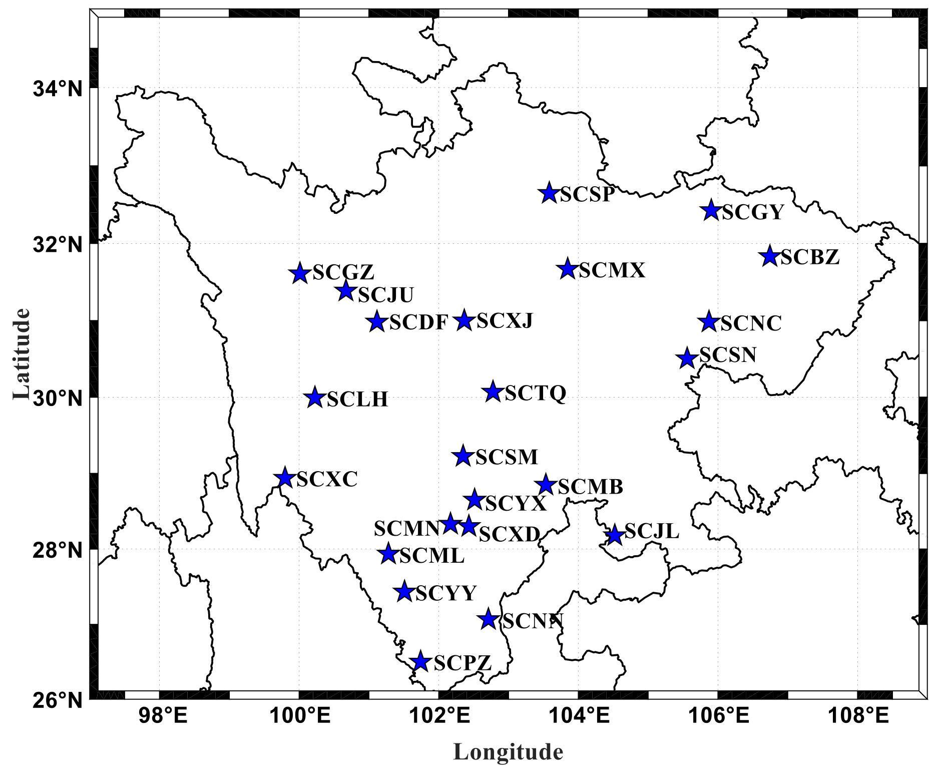
2.1. GNSS Data and Geomagnetic Activity Indices

The GNSS observations from the Crustal Movement Observation Network of China (CMONOC) is selected. There are 23 stations in Sichuan Province. The stations distribution is shown in Figure 1. The research time is from 3 July to 19 July 2013 (DOY184-DOY200), and the time resolution of the GNSS data is 30 s.

Solar activities and geomagnetic activities are two main causes for ionospheric disturbance. Dst, Kp, and F10.7 indexes can be used to evaluate the impacts of these two activities. The variation of the three indexes covering from DOY184 to DOY200 is shown in Figure 2. It can be seen from the figure that, before rainfall occurred, F10.7 was greater than 100 but less than 150 and showed a trend of increasing at the beginning and then decreasing. On DOY188, Dst < −70 nT and Kp > 4, which indicates the solar activities and geomagnetic activities were intense, while in the other days geomagnetic activities were relatively calm. After rainfall, F10.7 was decreasing and gradually turned to stable. On DOY190 (9 July 2013), the solar radiation was steady with 4.5% of its mean value (from DOY190 to DOY200). Dst was at a low level (−10 nT~10 nT) and Kp < 3, which indicated that the geomagnetic activity was weak. When the rainfall occurred, solar activities were less, and the geomagnetic field was relatively calm. Therefore, the ionospheric disturbance caused by solar activities and geomagnetic activities can be ignored, and the influence of heavy rainfall on the ionosphere should be the focus.

2.2. GNSS Data Processing Methods

Dual frequency GNSS receivers can record carrier phase measurements and code pseudo-range. The TEC sequences estimated by carrier phase measurements have a higher accuracy, but the ambiguities in carrier phase measurements are difficult to determine. Code pseudo-range measurements can be used to obtain absolute TEC sequences, with the accuracy of 1–5 TECU due to the high noise and multipath effects. Taking into account the characteristics of equal values and opposite signs of the ionospheric delays for phase measurements and code pseudo-range, the TEC can be estimated by combining the code pseudo-range and phase measurements in a continuous arc, which are called carrier phase smoothed pseudoranges [25].

The original observations of GNSS observations are as follows:

$$\begin{gathered} P_i=\rho +c(d{t}_{rcv}-d{t}^{sat})+Tr+{\alpha }_{i}I+b_{P_i,rcv}-b_{P_i}^{sat}+M+{\epsilon }_{Pi} \\ {L}_i=\rho +c(d{t}_{rcv}-d{t}^{sat})+Tr-{\alpha }_{i}I+b_{L_i,rcv}-b_{L_i}^{sat}+{\lambda }_i{N}_i+{\lambda }_{i}w+m_i+{\epsilon }_{Li} \end{gathered}$$

(1)

where, $P$ is the GNSS pseudorange measurement; $L$ is the GNSS carrier phase measurement; $i=1,2$ represents the frequency of observations $f_1$ and $f_2$, $f_1=1575.42\mathrm{MHz},f_2=1226.60\mathrm{MHz}$; $\rho$ is true distance between the GNSS receiver and satellite; $c$ is speed of light in a vacuum; $d{t}_{rcv}$ and $d{t}^{sat}$ are clock error of the receiver and the satellite, respectively; $Tr$ is troposphere delay; $a_{i}I$ is ionosphere delay ($a_i$ is the ionospheric delay coefficient, $a_i=\frac{40.3}{f_i^2}{10}^{16}{m}_{delay(signal{\varphi }_{f_i})}$); $b_{P_i,rcv}$ and $b_{P_i}^{sat}$ are the code delays for the satellite and receiver instrument biases, respectively; $b_{L_i,rcv}$ and $b_{L_i}^{sat}$ are the phase delays for the satellite and receiver instrument biases, respectively; $N$ is the ambiguity of the carrier phase, $w$ is the antenna Phase Wind-Up; $M$ and $m$ are the multipath effect of the pseudorange and phase, respectively; and $\epsilon$ are the residuals in the GNSS measurements.

The ionospheric delays can be obtained through dual-frequency observations:

$$\begin{gathered} P_4=P_1-P_2=(1-\frac{f_1^2}{f_2^2})I_1+c(DC{B}_r+DC{B}^s) \\ {L}_4=L_1-L_2=-(1-\frac{f_1^2}{f_2^2})I_1+c(b_r+b^s)+({\lambda }_1{N}_1-{\lambda }_2{N}_2) \end{gathered}$$

(2)

where, $P_4$ and $L_4$ are the geometry-free combination observations of the pseudorange and phase observations, respectively; $DC{B}_r=b_{P_1,rcv}-b_{P_2,rcv}$ and $DC{B}^s=b_{P_1}^{sat}-b_{P_2}^{sat}$ are differential code biases (DCB) of the receivers and satellites, respectively.

The ionospheric delay at L1 frequency can be expressed as:

$$I_1=\frac{40.3}{f_1^2}STEC$$

(3)

Combining the above equations, the slant total electron content (STEC) can be estimated with high accuracy [26,27].

$$STE{C}_N={\alpha }_0{P}_{4,sm}+{\alpha }_{0}c(DC{B}_r+DC{B}^s)$$

(4)

where, ${\alpha }_0=\frac{f_1^2{f}_2^2}{40.3(f_1^2-f_2^2)}$, $P_{4,sm}=(L_1-L_2)+\frac{1}{N}{\displaystyle \sum _{n=1}^N[(P_2-P_1)-(L_1-L_2)]}$, $N$ is the number of epochs in a continuous arc.

The details of the DCB estimation can be found in Jin et al. [28].

2.3. Time-Frequency Analysis Methods

According to the carrier phase smoothing code pseudo-range method, the STEC sequences can be obtained. The STEC series contain information such as background field information, disturbance signals and random noises, therefore, further processing is needed to extract the disturbance signals [29]. In our work, the noise in the data is removed using cubic smoothing spline method. A cubic spline is formed by using third-order polynomials which pass through a set of sample points. At the endpoints, the second derivative of each polynomial is set to zero.

The cubic smoothing spline estimate $f_S$ of the function $f$ is defined to be the minimizer of [30]:

$${\displaystyle \sum _{i=1}^n\{Y_i}-f_S(x_i){\}}^2+\eta {\displaystyle \underset{p}{\overset{q}{\int }}{f}_S^{″}(x)dx}$$

(5)

where $Y_i=f(x)+{\epsilon }_i$ is the $i\mathrm{th}$ set of $n$ observations in [p, q]; ${\epsilon }_i$ are independent zero mean random variables; and $\eta$ are the trade-off between data and smoothing.

When the differences between the STEC sequences and the smoothing sequences are less than the threshold, the final results are obtained. The method can detect the ionospheric disturbances clearly and get more continuous information with a high accuracy and stability [31,32].

In addition, the ionosphere is essentially a complex nonlinear system, which is manifested as multi-scale fluctuations and multi-frequency vibrations in time and space. Therefore, in this study, frequency domain analysis is also performed to obtain more effective signal information. With regard to studied ionosphere anomaly signals, we used the continuous wavelet transform (CWT) to effectively detect the instantaneous, singular and mutation components of non-stationary signal [33,34]. The outputs of the CWT provide both time and frequency information. The CWT is primarily defined as the inner products of a set of wavelets ${\Psi }_{u,s}(t)$ with the analyzed equation $f(t)$:

$$W(u,s)=\frac{1}{\sqrt{s}}{\displaystyle {\int }_{-\infty }^{+\infty }f(t){\Psi }^{*}}(\frac{t-u}{s})du$$

(6)

where, ${\Psi }_{u,s}(t)$ is a continuous function in both the time and the frequency domain called mother wavelet, ${\Psi }^{*}$ is the complex conjugate of ${\Psi }_{u,s}(t)$; $S$ and $u$ represent the dilation and translation parameters, respectively. In this work, the Morlet wavelet is used.

3. Results and Analysis

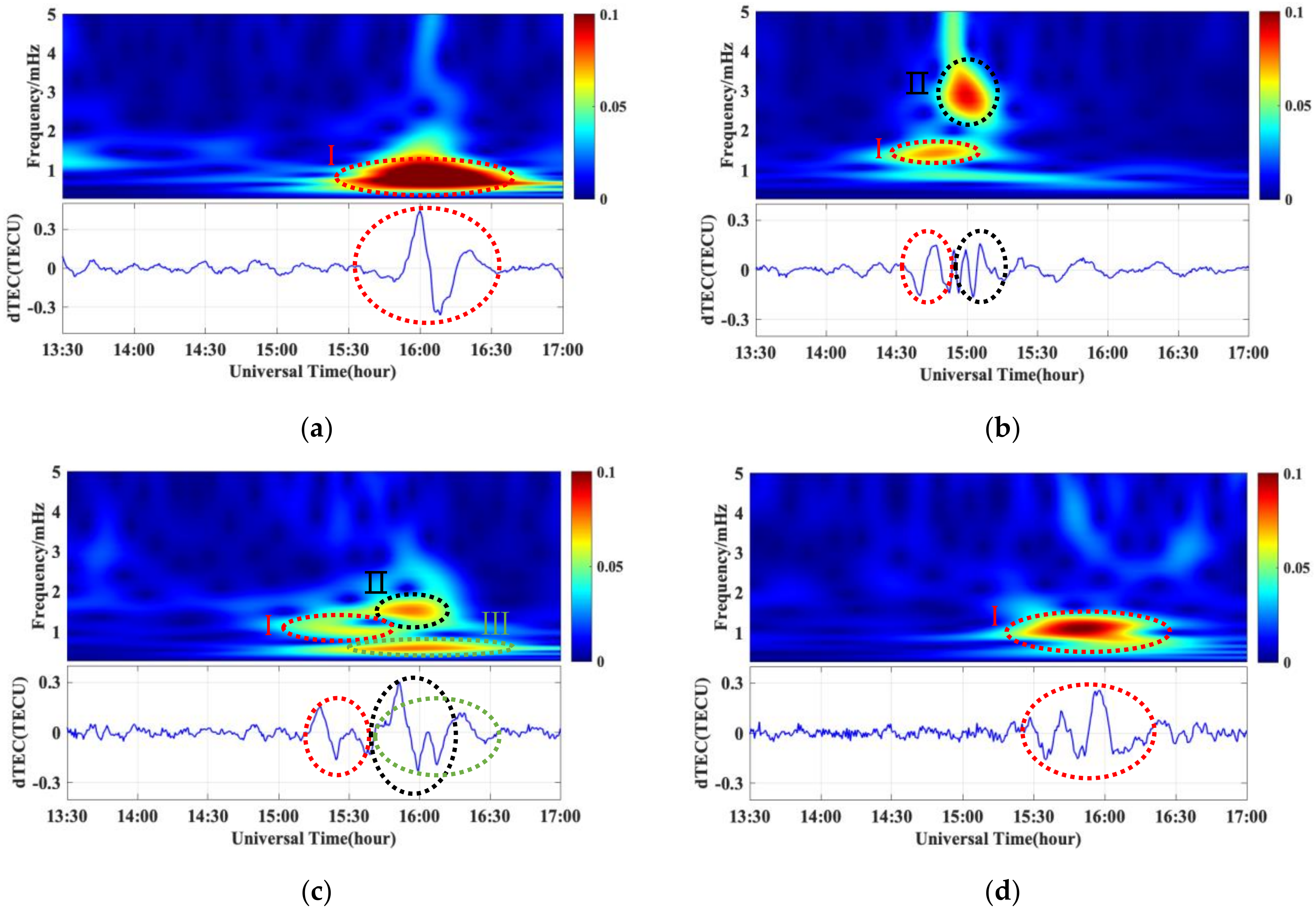
3.1. Time-Frequency Analysis of dTEC Sequences

To easily describe TEC variations, it is assumed that most of the ionospheric electrons are concentrated on an infinitely thin spherical shell at a certain height from the ground. This height is usually chosen to be 200–400 km, then an ionosphere monolayer model (Single Layer Model, SLM) can be established. When the positions of the GNSS stations and the satellites are determined, the points of intersection for the GNSS signal with the single ionosphere sphere are the Ionospheric Pierce Points (IPPs). Due to the non-periodic variation of the satellite orbit and the small variation of the Earth’s rotation speed, the IPP trajectory is almost the same every day. Therefore, ionospheric disturbances can be studied by calculating the trajectory of the IPPs over the research area and comparing the STEC variations in a period of time before and after the rainfall. Figure 3 shows some IPP trajectories corresponding to the stations (the IPP trajectories and orientation of all the 23 satellites corresponding to each station are calculated, due to limited space, Figure 3 only lists some IPP trajectories).

Using the data processing method in Section 2, the detrend TEC (dTEC) sequences were obtained. Taking the results observed by PRN5 as the example, and the dTEC sequences on DOY190 as shown in Figure 4 (each y grid denotes 0.5 TECU), it can be seen that, from UT14:00 to UT17:00, the dTEC sequences of each station showed obvious disturbances. Before the fluctuation occurred, the sequences were stable and fluctuated around 0 TECU. Then, the dTEC values began to increase, and the maximum reached to 0.4 TECU; after that, the values began to decline until to the lowest value, which is about −0.4 TECU. At the end of the fluctuation process, the dTEC sequences slowly turned to steady states. In the whole process, the TEC disturbances were similar to N-shaped waves. It can be clearly seen that there were time differences between disturbances arriving at each station, which indicated that the time of the disturbances arriving at each station was inconsistent and proved that there is a propagation processes of disturbances in the ionosphere.

Figure 5 shows the dTEC sequences of PRN5 observed at four random stations under the same period for 3 days. As the rainfall lasted for a long time, the dTEC sequences before and after the rainfall are selected (DOY185, DOY194 and DOY190). It can be seen that dTEC sequences on DOY190 had obvious disturbances between UT13:30 and UT17:00, up to the maximum of 0.4 TECU, while those on DOY185 and DOY194 fluctuated relatively calm in the same period, basically around 0 TECU, and without obvious disturbances.

Meanwhile, in order to analyze the dTEC sequences in the frequency domain, CWT is used to process the dTEC sequences and generate spectrograms to detect ionospheric disturbances and identify the disturbance time. Figure 6 gives the CWT results of dTEC sequences observed by PRN5. Several groups of representative spectrograms and their corresponding disturbance sequences are selected for analysis. The dark red part is the center frequency of the disturbances. It can be seen that, the wavelet energy density spectrums of ionospheric disturbance sequences have significant enhancements, and several anomalous spectrums of different frequencies can be seen during the studied period, which are basically in the range of 0.5–3 mHz [33].

For SCNN station, significant narrowband power around 0.5–1.5 mHz can be seen during UT15:30–16:30; For SCBZ station, there are two significant narrowband powers which are 1.2–1.7 mHz and 2–3 mHz, and corresponding start times of UT14:30 and UT14:50, respectively; For SCSM station, there are three significant narrowband powers which are 1–1.5 mHz, 1.5–2 mHz, and 0.5–0.8 mHz, which also corresponded to different abnormal start times; For the SCDF station, although the spectrogram is similar to the SCNN station, the intensity is not as strong as that of the SCNN station. Its narrowband power is about 1–1.5 mHz. From the dTEC sequence, it can be seen that the disturbance is the superposition of several signals with different amplitudes and periods, but these signal frequencies are relatively similar, the spectrogram cannot distinguish clearly.

The spectrum analysis indicate that the disturbance signal has different frequencies and intensity. Although some spectrum values are weak, they can still reflect ionospheric disturbance information. The analysis in frequency domain reached the same conclusion with the dTEC sequence in time domain: The dTEC sequences have obvious disturbances, and the time when the disturbance signals appear is inconsistent, showing the propagation characteristics of the disturbances in the atmosphere.

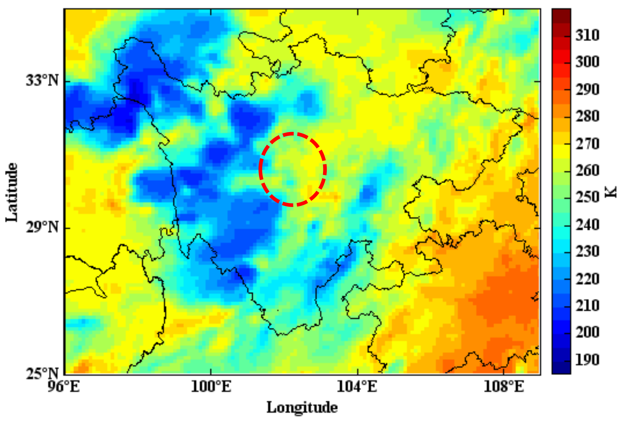
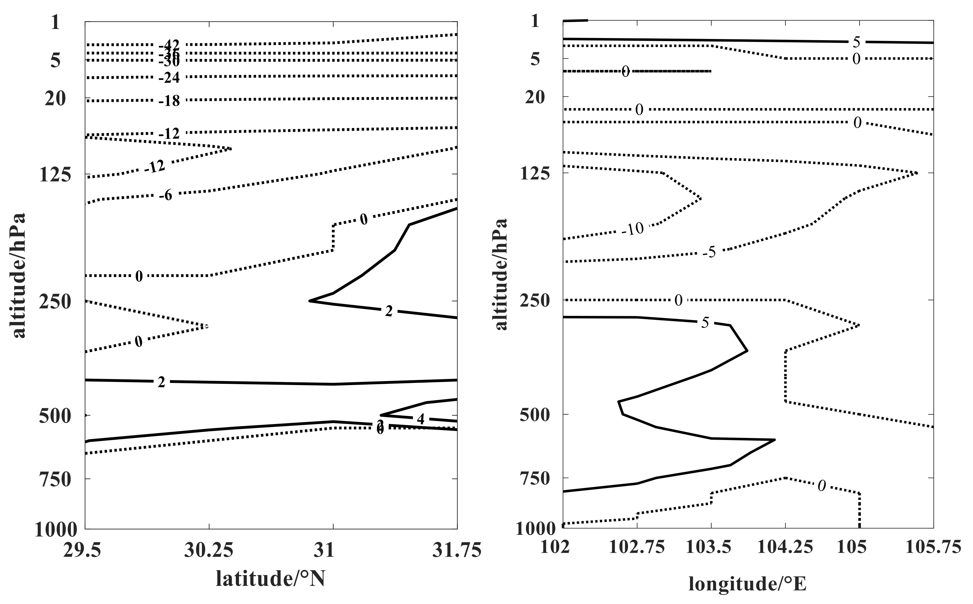
3.2. Searching the Trigger Source of Disturbances

The propagation directions of disturbances in the ionosphere are not unique, but in all directions. The triangulation process of feature points (IPPs) with three-station is applied to calculate propagation horizontal phase velocity and direction of the disturbances in the ionosphere [35]. The diagram illustrating the triangulation technique is shown in Figure 7. Because the coordinates and the time that disturbances reach the IPPs are estimated by processing GNSS observations, the coordinates and time difference that disturbances reach the feature points can be obtained. Then, a station (A) is selected as the origin to establish a coordinate system. D and E are the intersections of the perpendiculars from B and C to the direction of the disturbance propagation direction, respectively. Through the geometric relationship between the points, the horizontal propagation velocity and directions of the ionospheric disturbances can be calculated.

Similarly, every three stations can be used to get a horizontal velocity and propagation direction. Take the triangles formed by SCJU-SCXC-SCMN (the SCJU is the coordinate origin), SCMX-SCSN-SCGY (the SCMX is the coordinate origin) and SCLH-SCSM-SCSN (the SCLH is the coordinate origin) as the examples for the research. The distribution of the stations is shown in the Figure 8, and the propagation velocity information is shown in Figure 9. It can be seen that, for the three triangles, the average of horizontal phase velocity is about 143 m/s, 145 m/s, and 156 m/s, respectively, and average propagation azimuth is about −70°, 34°, and −85° respectively. Through the statistics of multiple combinations of the three-station triangles, the average of horizontal propagation phase velocity is about 150 m/s. Meanwhile, the extension lines of the three propagation directions intersect in an area, which is represented by a red triangle.

Multipoint observations can be used to detect the disturbances trigger source, so the trigger source on the earth surface can be determined by the grid searching method [19,36,37]. The principle is to divide the research area (Sichuan Province with longitude of 97°–109° and the latitude of 26°–35°) into 1° × 1° grids, and then search the locations that may excite the disturbances on a grid-by-grid basis.

Since the disturbances spread around in the atmosphere, the propagation routes are not fixed, but there are longest and shortest propagation distances. The longest distance is that the disturbances propagate vertically from the trigger source to the ionosphere, then propagate horizontally to the IPPs. The shortest distance is that the disturbances propagate radially in the atmosphere, and reach the IPPs directly. In this section, these two routes are discussed, which are shown as Route 1 and Route 2 in Figure 10.

Let the trigger source (the origin) coordinates be (X0, Y0) and the trigger time be $T_0$. P is the projection of the trigger source on the ionosphere single layer and its coordinates are (X, Y). P1, P2, P3 and P4 are IPPs, and their coordinates are (X1, Y1), (X2, Y2), (X3, Y3) and (X4, Y4) respectively, which can be calculated using GNSS observations.

For Route 1, the disturbances travel vertically to the ionosphere single layer at a propagation velocity of $v_1$.The disturbances horizontal propagation velocity in the ionosphere is $v_2=150\mathrm{m}/\mathrm{s}$. Then, the trigger source is obtained through the searching process, and the area that minimizes the time residual is regarded as the approximate location of the trigger source. The time residual is calculated as follows:

$$t1=T-(D_1/v_1+D_2/v_2)-T_0$$

(7)

where, $D_1$ is the vertical distance from the trigger source to the ionosphere single layer and is taken as 350 km in this paper. $D_2$ is the distance from P to IPPs which can be calculated according to the coordinates of two points. $T$ is the time when the disturbances reach the ionosphere.

For Route 2, the disturbances travel radially to the ionosphere IPPs at a radial propagation velocity $v_3$. The time residual is calculated as follows:

$$t2=T-D_3/v_3-T_0$$

(8)

where, $D_3$ is the straight-line distance from the trigger source to the IPPs, and $D_3=\sqrt{D_1^2+D_2^2}$.

When the absolute residual is at its minimum, it is considered to be the searching result, which is the trigger source of the disturbances. Figure 11 shows the distribution of the time residuals for the two routes. Both results are relatively consistent. The locations with the minimum absolute time residuals are in the central part of Sichuan Province, where there is the junction of the Sichuan Basin and the Qinghai-Tibet Plateau. The terrain here is undulating and height difference is large.

4. Discussion

Black Body Temperature (TBB) is usually referred to “cloud top brightness temperature”, which is a good indicator of the intensity of convective activity development [38]. In the cloud area, the lower the TBB value, the higher the cloud top and the stronger the convection. When TBB is < −20 °C (253.15 K), it indicates that strong convective activity is likely to occur. Figure 12 gives the TBB observations by FY-2E at UT12:00. At the trigger source (shown as the red circle), the TBB was about 250 K. And the TBB value in the western part of Sichuan Province was generally small, basically below 220 K, indicating that there was a strong convective activity. Moreover, it can be seen from Figure 4 that, the ionospheric disturbances had significant N-shaped waveform and propagation characteristic. Therefore, the ionospheric disturbances in this work are considered to be triggered by GWs under the effect of strong convective activities during the heavy rainfall. Due to the rapid dissipation of momentum and viscous interactions, strong convection is most likely to excite the GWs with various frequencies in the atmosphere [39].

GWs propagate in all directions in the atmosphere, and their propagation processes can transfer energy and momentum from the source region to another region, which leads to coupling between different layers of the atmosphere and causes atmospheric density disturbances [40,41,42]. Under proper atmospheric conditions (appropriate pressure and temperature, et al.), GWs can propagate up to the ionosphere and release energy there, thereby affecting the state of the ionosphere and causing ionospheric disturbances.

Topography also plays an important role in the propagation and development of the GWs. The topography of Sichuan Province is shown in Figure 13. Notably, the trigger source is located at the junction of the Sichuan Basin and the Qinghai-Tibet Plateau. There is a large difference in altitude, up to about 2000 m. Previous research has shown that the Qinghai-Tibet Plateau is an area usually with vigorous convection activities [43,44]. When strong convective weather occurs here, it is easy to excite the GWs. Mountains can also promote the upward propagation of GWs due to the blocking and reflecting effect. Moreover, the ground wind data provided by ECMWF ERA Interim on 9 July was used for analysis, as indicated by the blue arrows in Figure 13. It can be seen that, the ground wind in the trigger source was southeastward and it blew from the Sichuan Basin to the mountains. At the junction of the Sichuan basin and mountains, the wind turned to weak. Based on the energy conservation law, the horizontal wind there was considered to change into vertical wind, which promoted the upward propagation of the GWs.

The background wind field is also an important factor affecting the propagation of GWs. The background wind field has a filtering mechanism for GWs, which can reduce or increase the momentum flux carried by the waves, thereby affecting the propagation process. When the background wind field is going in the same direction as the GWs, it will reduce their momentum flux and slow down the motion of GWs. On the contrary, it will promote the propagation of GWs [45,46]. The relationship between the vertical wave number of the GWs and the vertical shear of the horizontal wind field given by the ray theory is shown in the following equation:

$$d{k}_z(z)/dt=-k_{x}d{u}_0(z)/dz$$

(9)

where, $k_x$ and $k_z$ are the horizontal and vertical wave numbers of GWs, respectively, $u_0$ is the background wind speed, $t$ is time, and $z$ is height.

When the GWs propagate upward, $k_z<0$. When $d{u}_0(z)/dz>0$, the vertical wave numbers of GWs decrease as the time increase, thus the vertical wavelength of the GWs is compressed; otherwise, when $d{u}_0(z)/dz<0$, the vertical wavelength of GWs will be stretched.

To explore the influences of background wind field on the GWs, the profile of zonal wind and meridional wind at the center of trigger source (104° E, 30° N) provided by ECMWF ERA Interim are shown in Figure 14. It can be seen that, the lower stratosphere was dominated by easterly wind, and the zonal wind produced a wind shear at 200 hPa. There was a strong westerly airflow in the stratosphere, with a maximum westerly wind speed of 45 m/s. While the meridional wind was northward from the near surface to the troposphere, and the lower stratosphere was a weaker southerly wind. The zonal wind velocity increased with height significantly larger than the meridional wind velocity. In addition, there were multiple wind shears in the zonal wind field, which would also affect the GWs. The intensity of the GWs is proportional to the vertical shear of the wind velocity, and increases as the vertical shear increases [47]. Therefore, the background wind field promotes propagation upward of GWs.

According to the law of conservation of energy, particle amplitude will continue to expand as atmospheric density decreases with height. However, GWs cannot continuously propagate upward in the vertical direction, and the maximum height is affected by the background wind field. When the GWs propagate above a certain height, strong dissipation occurs. The vertical wave number $m_{diss}$ with the maximum momentum flux of GWs is shown as follows [42]:

$$m_{diss}=\sqrt{(\frac{k_H{N}_B}{2H_{\rho }v})m_{diss}^{\frac{2}{5}}-K_H^2-\frac{1}{4H_{\rho }^2}}$$

(10)

where, $k_H$ is the horizontal wave number, $N_B$ is the Brunt frequency, $v$ is the molecular viscosity coefficient, and $H_{\rho }$ is the scale height.

We assume that GWs are induced at a height near the top of the troposphere (about 12 km), and the horizontal wavelength at the height of the stratosphere (40 km) is 2π/200 km, then according to above formula, it can be calculated that the dissipative height of GWs is about 400 km. It shows that the GWs excited during the rainfall can propagate to the height of the F2 layer of the ionosphere.

During the rainfall, GWs may be excited in lower atmosphere. When GWs propagate upwards, their amplitude and wave flux increase rapidly as the altitude increase when there is no attenuation. Otherwise, the GWs diverge their momentum into the airflow and form a coupling effect between the bottom atmosphere and the upper atmosphere. After the GWs reach the ionosphere, the energy released by the breaking of GWs will cause disturbances in the background wind field and atmospheric temperature, which will directly affect the collision rate of neutral particles and ions in the ionosphere [48]. When ions oscillate in the direction of the magnetic field line, the electrons will also oscillate, thereby generating a disturbance of the electron density in the ionosphere. In addition, the process of GWs dissipating in the ionosphere would cause temperature changes, which affect the efficiency of the chemical reactions of electrons, thereby changing the distribution of electrons and causing disturbances in the ionosphere.

5. Conclusions

In this paper, the ionospheric disturbances responding to a heavy rainfall in Sichuan Province is discussed. The STEC can be estimated with high precision from GNSS observations by using carrier phase smoothed pseudoranges method. The STEC is then processed by a cubic smoothing spline to obtain the dTEC sequence. The main conclusions are as follows:

(1)

The time domain and frequency domain analysis of dTEC sequences both show obvious ionospheric disturbances with a maximum amplitude of 0.4 TEC and frequencies between 0.5–3 mHz.

(2)

The horizontal propagation velocity of ionospheric disturbances is about 150 m/s. Then the disturbances trigger source is determined to be the central part of Sichuan Province using the grid searching method.

(3)

It can be seen from the FY-2E TBB that there may be a strong convection at the trigger source. The strong convection during the rainfall excited GWs in the atmosphere. Under the promotion of topography, background wind field, and other factors, the GWs propagated in the atmosphere along the horizontal and vertical directions. When the GWs reached a certain height, they would break and deposit their momentum and energy into the background atmosphere, causing disturbances in the stratosphere and ionosphere.

The GWs play a significant role in the transport of energy and momentum from the lower atmosphere to the ionosphere. After the GWs break, they deposit their momentum and energy into the background atmosphere. This will cause the background wind to accelerate along the wave propagation direction, thereby changing the atmospheric dynamic structure, atmospheric circulation, and atmospheric thermodynamic structure. This mechanism is an important way for lower atmospheric activities to affect the state of the middle and upper atmosphere, which plays an important role in their energy balance. The study confirms that meteorological activities in the lower atmosphere will have an impact on the ionosphere, and provides support for in-depth exploration of the troposphere-ionosphere coupling mechanism.

References

1. Cang, Z.; Cheng, G.; Cheng, G. Ionospheric anomalous disturbance during the tropospheric strong convective weather. J. Atmos. Solar-Terr. Phys. 2015, 129, 55–61. [Google Scholar] [CrossRef]
2. Lastovicka, J. Lower ionosphere response to external forcing: A brief review. Adv. Space Res. 2009, 43, 1–14. [Google Scholar] [CrossRef]
3. Kazimirovsky, E.; Herraiz, M.; Morena, B.A. Effects on the ionosphere due to phenomena occurring below it. Surv. Geophys. 2003, 24, 139–184. [Google Scholar] [CrossRef]
4. Rishbeth, H. F-region links with the lower atmosphere? J. Atmos. Solar-Terr. Phys. 2006, 68, 469–478. [Google Scholar] [CrossRef]
5. Lastovicka, J. Forcing of the ionosphere by waves from below. J. Atmos. Solar-Terr. Phys. 2006, 68, 479–497. [Google Scholar] [CrossRef]
6. Beynon, W.J.G.; Brown, G.M. Geophysical and meteorological changes in the period Junuary-April 1949. Nature 1951, 167, 1012–1014. [Google Scholar] [CrossRef]
7. Bauer, S.J. A possible troposphere-ionosphere relationship. J. Geophys. Res. 1957, 62, 425–430. [Google Scholar] [CrossRef]
8. Baker, D.M.; Davies, K. F2-region acoustic waves from severe weather. J. Atmos. Terr. Phys. 1969, 31, 1345–1352. [Google Scholar] [CrossRef]
9. Shrestha, K.L. Sporadic-E and atmospheric pressure waves. J. Atmos. Terr. Phys. 1970, 33, 205–211. [Google Scholar] [CrossRef]
10. Shen, C. The correlations between the typhoon and the f0F2 of ionosphere. Chin. J. Space Sci. 1982, 2, 335–340. [Google Scholar]
11. Xu, G.; Wan, W.; Ning, B. Effects of extreme heavy rainfall in the troposphere on the ionosphere. Chin. J. Space Sci. 2005, 25, 104–110. [Google Scholar]
12. Mao, T.; Wang, J.; Yang, G.; Tao, Y.; Ping, J.; Suo, Y. Effects of typhoon Matsa on ionospheric TEC. Chin. Sci. Bull. 2010, 8, 712–717. [Google Scholar] [CrossRef]
13. Hung, R.; Lee, C.C.; Johnson, D.L.; Chen, A. Remote sensing of mesospheric and thermospheric density perturbations induced by subtropical heavy rainfalls for spacecraft environment study. Acta Astronaut. 1991, 25, 379–393. [Google Scholar] [CrossRef]
14. Tsutsui, M.; Ogawa, T. HF Doppler observation of ionospheric effects due to typhoons. Rep. Ionos. Space Res. Jpn. 1973, 27, 121–123. [Google Scholar]
15. Xiao, S.; Hao, Y.; Zhang, D.; Xiao, Z. A case study on whole respond processes of the ionosphere to typhoons. Chin. J. Geophys. 2006, 49, 623–628. [Google Scholar] [CrossRef]
16. Zhang, Y.; Chen, H.; Li, C. Correlation analysis between ionospheric TEC and ground weather parameters during cold wave. J. Nanjing Univ. Inf. Sci. Technol. 2013, 5, 278–283. [Google Scholar]
17. Liu, J.; Tsai, Y.B.; Ma, K.; Chen, Y.; Tsai, H.F.; Lin, C.; Masashi, K.; Lee, C.P. Ionospheric GPS total electron content (TEC) disturbances triggered by the 26 December 2004 Indian Ocean tsunami. J. Geophys. Res. Space Phys. 2006, 111, A5. [Google Scholar] [CrossRef] [Green Version]
18. Yang, Z.; Liu, Z. Observational study of ionospheric irregularities and GPS scintillations associated with the 2012 tropical cyclone Tembin passing Hong Kong. J. Geophys. Res. Space Phys. 2016, 121, 4705–4717. [Google Scholar] [CrossRef]
19. Kong, J.; Yao, Y.; Xu, Y.; Zhang, L.; Liu, L.; Zhai, C. A clear link connecting the troposphere and ionosphere: Ionosphere response to the 2015 Typhoon Dujuan. J. Geod. 2017, 91, 1087–1097. [Google Scholar] [CrossRef]
20. Rastogi, R.G. Thunderstorms and sporadic- E layer ionization over Ottawa, Canada. J. Atmos. Terr. Phys. 1961, 24, 533–540. [Google Scholar] [CrossRef]
21. Ma, X.; Yu, K.; Montillet, J.P.; He, X. One-step solution to local tie vector determination at co-located GNSS/VLBI sites. Stud. Geophys. Geod. 2018, 62, 535–561. [Google Scholar] [CrossRef]
22. Liu, Y.; Wang, J.; Xiao, Z.; Suo, Y. A possible mechanism of typhoon effects on the ionospheric layer. Chin. J. Space Sci. 2006, 26, 92–97. [Google Scholar]
23. Shan, L.; Yao, Y. Analysis of Ionospheric Anomalous Disturbance during a Heavy Rainfall. In China Satellite Navigation Conference (CSNC) 2018 Proceedings; Lecture Notes in Electrical Engineering; Sun, J., Yang, C., Guo, S., Eds.; Springer: Singapore, 2018; pp. 233–242. [Google Scholar]
24. Shi, R.; Chen, Y.; Xiao, H. Comparative Analysis of Continuous Rainstorm in Sichuan Basin in 2013. Plateau Mt. Meteorol. Res. 2014, 34, 11–15. [Google Scholar]
25. Yuan, Y.; Huo, X.; Zhang, B. Research progress of precise models and correction for GNSS ionospheric delay in China over recent years. Acta Geod. Cartogr. Sinica. 2017, 46, 1364–1378. [Google Scholar]
26. Liu, Z.; Gao, Y.; Skone, S. A study of smoothed TEC precision inferred from GPS measurements. Earth Planets Space 2005, 57, 999–1007. [Google Scholar] [CrossRef] [Green Version]
27. Yao, Y.; Zhai, C.; Kong, J.; Zhao, C.; Luo, Y.; Liu, L. An improved constrained simultaneous iterative reconstruction technique for ionospheric tomography. GPS Solut. 2020, 24, 68. [Google Scholar] [CrossRef]
28. Jin, R.; Jin, S.; Feng, G. M_DCB: Matlab code for estimating GNSS satellite and receiver differential code biases. GPS Solut. 2012, 16, 541–548. [Google Scholar] [CrossRef]
29. He, X.; Montillet, J.-P.; Fernandes, R.; Bos, M.; Yu, K.; Hua, X.; Jiang, W. Review of current GPS methodologies for producing accurate time series and their error sources. J. Geod. 2017, 106, 12–29. [Google Scholar] [CrossRef]
30. Dierckx, P. An algorithm for smoothing, differentiation and integration of experimental data using spline functions. J. Comput Appl Math. 1975, 1, 165–184. [Google Scholar] [CrossRef] [Green Version]
31. Maletckii, B.; Yasyukevich, Y.; Vesnin, A. Wave Signatures in Total Electron Content Variations: Filtering Problems. Remote Sens. 2020, 12, 1340. [Google Scholar] [CrossRef] [Green Version]
32. Yasyukevich, Y.V.; Kiselev, A.V.; Zhivetiev, I.V.; Edemskiy, I.K.; Syrovatskii, S.V.; Maletckii, B.M.; Vesnin, A.M. SIMuRG: System for Ionosphere Monitoring and Research from GNSS. GPS Solut. 2020, 24, 69. [Google Scholar] [CrossRef]
33. Zhai, C.; Shi, X.; Wang, W.; Hartinger, M.D.; Yao, Y.; Peng, W.; Lin, D.; Ruohoniemi, J.M.; Baker, J.B.H. Characterization of high-m ULF wave signatures in GPS TEC data. Geophys. Res. Letters. 2021, 48, 14. [Google Scholar] [CrossRef]
34. He, L.; Wu, L.; Liu, S.; Ma, B. Seismo-ionospheric anomalies detection based on integrated wavelet. In Proceedings of the 2011 IEEE International Geoscience and Remote Sensing Symposium, IGARSS 2011, Vancouver, BC, Canada, 24–29 July 2011. [Google Scholar]
35. Waston, C.; Jayachandran, P.T.; Spanswick, E.; Donovan, E.F.; Danskin, D.W. GPS TEC technique for observation of the evolution of substrom particle injection. J. Geophys. Res. 2011, 116, A00190. [Google Scholar]
36. Lee, W.H.K.; Lahr, J.C. HYPO71: A Computer Program for Determining Hypocenter, Magnitude, and First Motion Pattern of Local Earthquakes; Open File Report 75-311; U.S. Geological Survey: Reston, VA, USA, 1975; pp. 1–116.
37. Liu, J.; Tsai, H.F.; Lin, C.; Kamogawa, M.; Chen, Y.; Huang, B.; Yu, S.; Yeh, Y.L. Coseismic ionospheric disturbances triggered by the Chi-Chi earthquake. J. Geophys. Res. Atmos. 2010, 115, A8. [Google Scholar] [CrossRef]
38. Vadas, S.L.; Fritts, D.C. Reconstruction of the gravity wave field from convective plumes via ray tracing. Ann. Geophys. 2009, 27, 147–177. [Google Scholar] [CrossRef] [Green Version]
39. Xu, J.; Li, Q.; Yue, J.; Hoffmann, L.; Straka, W.C., III; Wang, C.; Liu, M.; Yuan, W.; Han, S.; Miller, S.D.; et al. Concentric GWs over northern China observed by an airglow imager network and satellites. J. Geophys. Res. Atmos. 2015, 120, 11058–11078. [Google Scholar] [CrossRef] [Green Version]
40. Xiao, Z.; Xiao, S.; Hao, Y.; Zhang, D. Meteorological features of ionospheric response to typhoon. J. Geophys. Res. Space Phys. 2007, 112, A4. [Google Scholar] [CrossRef] [Green Version]
41. Tsugawa, T.; Saito, A.; Otsuka, Y.; Nishioka, M.; Maruyama, T.; Kato, H.; Nagatsuma, T.; Murata, K.T. Ionospheric disturbances detected by GPS total electron content observation after the 2011 off the Pacific coast of Tohoku Earthquake. Earth Planets Sp. 2011, 63, 875–879. [Google Scholar] [CrossRef] [Green Version]
42. Vadas, S.L. Horizontal and vertical propagation and dissipation of GWs in the thermosphere from lower atmospheric and thermospheric source. J. Geophys. Res. 2007, 112, A6. [Google Scholar]
43. Hoffmann, L.; Xue, X.; Alevander, M.J. A global view of stratospheric gravity wave hotpots located with Atmospheric Infrared Sounder observations. J. Geophys. Res. Atmos. 2013, 118, 416–434. [Google Scholar] [CrossRef] [Green Version]
44. Li, J.; Li, L.; Wu, Z.; Wan, W.; Ning, B. Ionospheric disturbances related to the meteorology of Qinghai-Xizang Plateau. Publ. Yunnan Obs. 1990, 1, 1. [Google Scholar]
45. Vadas, S.L.; Nicolls, M.J. Temporal evolution of neutral, thermosphere winds and plasma response using PFISR measurements of GWs. J. Atmos. Sol. Terr. Phys. 2009, 71, 740–770. [Google Scholar] [CrossRef]
46. Vadas, S.L.; Liu, H. Generation of large-scale GWs and neutral winds in the thermosphere from the dissipation of convectively generated GWs. J. Geophys. Res. 2009, 114, A10. [Google Scholar]
47. Beres, H.J.; Alexander, J.M.; Holton, J.R. Effects of tropospheric wind shear on the spectrum of convectively generated GWs. J. Atmos. Sci. 2002, 59, 1805–1824. [Google Scholar] [CrossRef] [Green Version]
48. Yiğit, E.; Knížová, P.K.; Georgieva, K.; Ward, W. A review of vertical coupling in the Atmosphere–Ionosphere system: Effects of waves, sudden stratospheric warmings, space weather, and of solar activity. J. Atmos. Solar-Terr. Phys. 2016, 141, 1–12. [Google Scholar] [CrossRef]
Figure 1. The distribution of CMONOC stations in Sichuan Province.
Remotesensing 14 00510 g001
Figure 2. Kp, Dst, and F10.7 indexes covering from DOY184 to DOY200.
Remotesensing 14 00510 g002
Figure 3. IPP trajectories corresponding to the stations (The distribution of the GNSS stations in is shown with black triangle, and the IPP trajectories are represented by different colors).
Remotesensing 14 00510 g003
Figure 4. dTEC sequences of PRN5 from 23 stations on DOY190 (each y grid denotes 0.5 TECU).
Remotesensing 14 00510 g004
Figure 5. dTEC sequences of PRN5 at 4 stations on different three day (DOY185, DOY194 and DOY190); (a) SCGZ; (b) SCNC; (c) SCNN; (d) SCYX.
Remotesensing 14 00510 g005
Figure 6. The results of CWT for ionospheric dTEC observed by PRN5 on DOY190; (a) SCNN station; (b) SCBZ station; (c) SCSM station; (d) SCDF station.
Remotesensing 14 00510 g006
Figure 7. Diagram illustrating the triangulation technique for calculating the horizontal propagation velocity of the ionospheric disturbances.
Remotesensing 14 00510 g007
Figure 8. The distribution of the three triangles used in triangulation technique and propagation information (The black five-pointed star represents the location of the stations, and each triangle is connected by a different colored line).
Remotesensing 14 00510 g008
Figure 9. The horizontal phase velocity and azimuth of disturbances propagating in the ionosphere by using the SCJU-SCXC-SCMN, SCMX-SCSN-SCGY, and SCLH-SCSM-SCSN, respectively; (a) The horizontal phase velocity by using SCJU-SCXC-SCMN; (b) the azimuth by using SCJU-SCXC-SCMN; (c) The horizontal phase velocity by using SCMX-SCSN-SCGY; (d)the azimuth by using SCMX-SCSN-SCGY; (e) The horizontal phase velocity by using SCLH-SCSM-SCSN; (f) the azimuth by using SCLH-SCSM-SCSN.
Remotesensing 14 00510 g009
Figure 10. Two main propagation routes with the longest distance and the shortest distance.
Remotesensing 14 00510 g010
Figure 11. The disturbances trigger source obtained by searching method; (a) Route1 results; (b) Route2 results.
Remotesensing 14 00510 g011
Figure 12. FY-2E observations of cloud top brightness temperature at UT12:00 on 9 July 2013 (The red circle is the location of the trigger source).
Remotesensing 14 00510 g012
Figure 13. The topographic map of Sichuan Province within the wind information at UT12:00 on 9 July (The red circle is the location of the trigger source).
Remotesensing 14 00510 g013
Figure 14. Zonal wind (left, east wind is positive) and meridional wind (right, north wind is positive) at different constant-pressure altitudes above the trigger source at UT12:00 on 9 July.
Remotesensing 14 00510 g014
Publisher’s Note: MDPI stays neutral with regard to jurisdictional claims in published maps and institutional affiliations.