Abstract
By using fast ionogram observations, we report the first simultaneous observations of ascending ion layers at equatorial and low latitudes. The ionosonde measurements at Sanya (18.3°N, 109.6°E; dip lat. 12.2°N) and Chumphon (10.7°N, 99.4°E; dip lat. 3.8°N) show that a high Es layer, which might contain metallic ions, was directly lifted upward from the local E region to F region bottomside at morning hours, in a pattern similar to the vertical drift of the F region background ionosphere driven by the daytime eastward electric field. A statistical analysis with Sanya ionosonde measurements shows that the low latitude ascending ion layer is not a rare phenomenon, with a maximum occurrence of 22% during equinox. The results indicate that at the latitudes far away from the magnetic equator, the local E region metallic ions could be directly brought into the F region with the ascending layer. It can be expected that fast ionogram measurements, which can easily capture the rapid evolution of the background ionosphere, will play an important role in studying the formation of some unexpected high altitude metallic layers.
1. Introduction
The ionosphere is the medium of radio wave propagation. In addition to the regular variations in the background ionosphere, there are some special phenomena and structures in the ionosphere, such as sporadic E (Es), equatorial plasma bubble, spread F, etc. They can cause scintillation and loss of locks of the radio wave signals propagating through the ionosphere and seriously affect the reliability of communication and navigation, positioning, and other high-tech systems relying on the trans-ionospheric propagation services [1,2,3,4]. Es layers are thin and highly dense plasma layers appearing in the lower ionosphere. They can become denser than the normal E layer or even the peak F layer [5]. Es layers were studied extensively for decades using rocket and satellite in situ measurements, as well as incoherent scatter radar (ISR) and ionosonde observations [6,7,8,9].
Rocket measurements showed that the Es layer was mainly comprised of metallic ions. The dominant E-region ion O+ was not detected within the Es layer during the flight of the rocket [6,7]. Ground-based observations could trace the vertical motion of the Es layer. ISR is a powerful instrument to monitor the ionospheric structure with superb sensitivity and good range and time resolution. Statistical results from 14 years of Arecibo ISR observations showed that the Es layer generally descended in a diurnal and semidiurnal periodicity [8]. Based on ionosonde observation at Chung-li, an equatorial anomaly station, the occurrence and vertical motion of higher Es layers were studied. Statistical results indicated that Es layers appeared primarily during the daytime in the spring/winter months. The layers descended from high to low altitudes and different tidal motions controlled the layers in different seasons [10]. At mid-latitude, a method of height-time-frequency analysis was applied on the ionogram recorded at Milos (36.7°N, 24.5°E) to study the vertical motion of the Es layers with high temporal resolution ionograms (5 min/2 min during the daytime/nighttime) [9]. The Es layer was characterized by a daytime layer at 120 km and a nighttime layer at above 125 km, of which both moved downward but with a higher descending rate during nighttime. This method was recently applied to study the daily and seasonal variability of Es layers over three European stations. A 12 h periodicity prevailed throughout the year, while 6 h and 8 h periodicities were also found in winter and summer, respectively [11]. In the Brazil sector, the occurrence frequency of the descending Es layer is >60% over São Luís and >90% over Cachoeira Paulista. In most cases, the layers occur during the day at altitudes 130–180 km and descend to lower altitudes [12].
It is now generally accepted that the Es layers are majorly composed of metallic ions through a wind shear mechanism [5,13]. The long-lived metallic ions move vertically and converge into thin and dense plasma layers when meridional winds are poleward (upside) and equatorward (downside) and zonal winds are eastward (downside) and westward (upside) in the northern hemisphere through the combined action of ion-neutral collisional coupling and geomagnetic Lorentz forcing [5]. The atmospheric tides primarily produce the vertical shears of horizontal winds and cause the Es layers to descend with the downward propagations of the tide phases. The ions composing Es layers are suggested to be metallic (monoatomic) ions of a meteoric origin undergoing slow radiative recombination, since Es layers live a long time while ambient molecular ions live a short time due to dissociative recombination [5,13].
For the observed descending Es layers, their initial heights were much higher than the general heights of meteor ablation, 90–110 km. The results raise a question: what is the source of these high altitude Es layers and how do they appear at such high altitudes? Hanson and Sanitani [14] suggested a possibility that the E × B drift driven by the equatorial dynamo electric field was the active agent, which lifts the E region metallic ions to higher altitudes around the magnetic equator. For the lifted metallic ions around the magnetic equator, the fountain effect takes over and transports the ions, via gravity and diffusion, to higher latitudes along the magnetic field lines. The deposit of metallic ions from the equatorial F region to low latitudes via the fountain effect provides the metallic ions in the thermosphere. Later numerical simulations confirmed the electric field control in the formation of high altitude metallic ions [15,16,17,18].
Whereas the previous theoretical and model simulation studies have shown that the high altitude metallic ions are sourced from the equatorial E region, there is almost no direct observational evidence of the upward transport of metallic ions from the E region to F region. To our best knowledge, only two cases of ascending thin layer events were briefly reported, at Jicamarca [19] and São Luís [12]. However, the ascending rates of thin layers were quite fast, and the whole evolving process of the thin layers was not very clear due to the low time resolution of the ionograms in these two cases (30 min/10 min for the Jicamarca case and São Luís case, respectively). In this context, an ionosonde with the capability to detect ionospheric variations with high time/height resolution could provide more insight to the vertical motion of the thin layer.
In this paper, a large database of rapid-run ionosonde observations at low latitude Sanya (18.3°N, 109.6°E; dip lat. 12.2°N) during the periods December 2017–June 2018 and April 2019–June 2020 are investigated. Together with the equatorial ionosonde measurements at Chumphon (10.7°N, 99.4°E; dip lat. 3.8°N), we report thin layers ascending from the E region to the F region, simultaneously observed at low latitude and the magnetic equator for the first time. A statistical analysis shows that the low latitude ascending ion layer is not a rare phenomenon. In addition to the equatorial fountain effect, our results suggest a new possibility that the low latitude F region metallic ions could be directly from the local E region. This may have important implications for understanding the sources of the high altitude metallic layers reported previously.
2. Materials and Methods
According to Christakis et al. [8] and Haldoupis et al. [9], high temporal resolution observations are conducive to studying the evolution of the Es layer. In this regard, the portable digital ionosonde (PDI) was designed to carry out long-term unattended fast (with a time interval less than 1 min) ionogram observation [20]. Two techniques are employed in PDI to acquire high time resolution ionograms/Doppler-ionograms: (1) The complementary code pulse multiplexing. PDI uses the current pulse together with one of the previous pair of pulses to form a new pair of pulses and to eliminate the side lobes. (2) Polarization separation by software. The PDI antenna radiates a linearly polarized electromagnetic wave. The polarized wave will be split into the ordinary (O) and the extraordinary (X) waves in the ionosphere and both are received by the two crossed receiving antennas. The O and X waves are then separated by software calculation. For more details concerning the PDI ionosonde, please refer to Lan et al. [20]. As a result, the PDI can operate nearly 4 times as fast as a typical ionosonde such as DPS4D under the same detecting settings. For example, a PDI ionosonde is capable of completing 1–16 MHz sweeping with a 50 kHz frequency step and an 80–1200 detecting range with 16 times coherent integration in ~50 s, while the time needed for a DPS4D ionosonde is more than 3 min with the same settings. The PDI was used for regular ionospheric vertical sounding at a cadence of 1 min/2 min at Sanya. During the periods December 2017–June 2018 and April 2019–June 2020, the data were recorded for a total of 144 and 367 days, respectively. The PDI was operated with the frequency ranging 1–16 MHz (or 1–25 MHz) with a step of 50 kHz in a time interval of 1 min (or 2 min). A total of 1440 (or 720) individual ionograms were recorded each day.
The ionosonde data at Chumphon (10.7°N, 99.4°E, dip lat. 3.8°N), which is located near the magnetic equator and belongs to the Southeast Asia Low Latitude Ionosphere Observation Network (SEALION) [21], were used. The Chumphon ionosonde is a portable low power FMCW ionosonde [22]. The operational frequency ranges 2–30 MHz. The temporal resolution of ionograms is 5 min. The ionosonde observations at Sanya and Chumphon with 1 min/2 min and 5 min cadence, which are generally faster than those of the digisonde observations made at Jicamarca [19] and São Luís [12], provide more details on the temporal variation of Es layer.
3. Results and Discussion
Figure 1 presents a sequence of ionograms extracted from the 1 min resolution ionograms on 4 April 2018 (LT = UT + 7 h 18 min), a geomagnetic quiet day with a sum of Kp 8.3. Similar to the ionogram scaling in previous studies [23], here the ordinary wave traces were used to determine the electron density profile. As shown in the figure, two types of Es layers, the low Es in the virtual height of ~110 km (indicated by L) and the high Es in the virtual height of 145–190 km (indicated by H) occurred in the ionogram at 0230 UT (0948LT). We focus on the high Es layer, which shows obvious upward drift in later hours and is, thus, named the ascending ion layer. During 0245–0314 UT, the shape of the ascending layer showed obvious changes, with an evident cusp structure. The minimum virtual height of the structure increased to 200 km at 0314 UT, being connected with the F1 layer trace. In order to present the movement, we marked the position of the high Es layer with a black arrow pointing to the turning point in F1 layer trace. The true height of the ascending ion layer can be calculated by the electron density profile inversion algorithm (NHPC) embedded in the SAOExplorer software [24]. As indicated by the arrows in panel g, the virtual height and true height of the ion layer are about 217 km and 141 km, respectively. The ion layer continued ascending from a virtual height of 217 km at 0330 UT to 292 km at 0400 UT and finally disappeared at 0432 UT (1150 LT). The frequency at the turning point labeled with the black arrow also increased from 3.9 MHz to 4.4 MHz during 0307–0400 UT. This frequency, however, is actually the combined effect of background electron density and the Es layer density. During 0300–0400UT, it appeared that the F1 layer disappeared between 0314–0330UT. Actually, the fact is that the upper part of the F1 layer trace, which is higher than the high Es layer, became steeper as the high Es layer ascended. This made the F1 layer trace appear to break off due to the limited frequency resolution of the ionogram. An animation of ionograms (S1) obtained during the period 2200 UT, 3 April-0500UT, 4 April is provided in the data repository of this paper at https://doi.org/10.12197/2022GA006 (last accessed 25 October 2022). It clearly shows the detailed evolution of the ascending ion layer. At the nearby site Fuke (19.5°N, 109.1°E; dip lat. 13.4°N), the ascending ion layer was also observed in the 15 min resolution ionograms (Figure S2 in data repository).
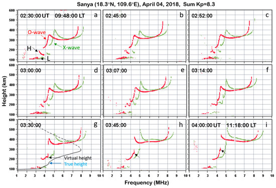
Figure 1.
The ionograms observed at Sanya during 0230–0400UT (0948–1118LT) on 4 April 2018 (a–i). The letters L and H in panel (a) denote low and high altitude Es layer traces, respectively. The red and green traces in the ionograms represent the ordinary wave (O-wave) and extraordinary wave (X-wave), respectively. The black arrows in panels (g–i) denote the ascending ion layer. The blue arrow in panel (g) indicates the true height of the ascending ion layer in the calculated ionospheric electron density profile.
In order to obtain the whole evolution process of the ascending ion layer, the ionograms were manually scaled with the SAOExplorer software [23]. The ordinary wave traces and ionospheric parameters (e.g., virtual height, true height) were retrieved. As shown in Figure 2a, the ion layer (indicated by the red circles) started to ascend at 0210 UT and reached the peak virtual height at 0425 UT. During this period, the F2 layer height also showed an ascending trend. Figure 2b shows the summary plot of the manually scaled ordinary wave trace with a time resolution of 1 min (different plasma frequencies are color-coded) during the period 2200 UT, 3 April–0500 UT, 4 April (0518–1218 LT, 4 April). The virtual height of the ascending ion layer is marked by red dots. A low Es layer appeared steadily in the virtual heights of 105–120 km with plasma frequencies of 1.5–3 MHz. The high Es layer initially appeared at 2240 UT, 3 April (0558 LT of 4 April), with a critical frequency of 1.6 MHz. It ascended from the upper E region to the F region, shown as a rising structure in the plot. Before ~0200 UT, the virtual height of the ion layer did not change much, except around 0100 UT when a slight enhancement was observed. The variation of the F layer virtual height around the plasma frequencies 3–4 MHz also showed a slight enhancement, similar to that of the high Es layer. After 0200 UT, the ion layer started to move upward, connected to the F1 layer trace at 0310 UT, and reached the maximum virtual height of 510 km at 0422 UT when it moved to the F1 ledge. The virtual height of the ion layer decreased as it continued moving to the F2 layer. Finally, the ion layer disappeared in the F2 layer trace at 0432 UT. During the ascending of the ion layer, the F layer virtual height (around the plasma frequencies 4–6 MHz) also increased slowly.
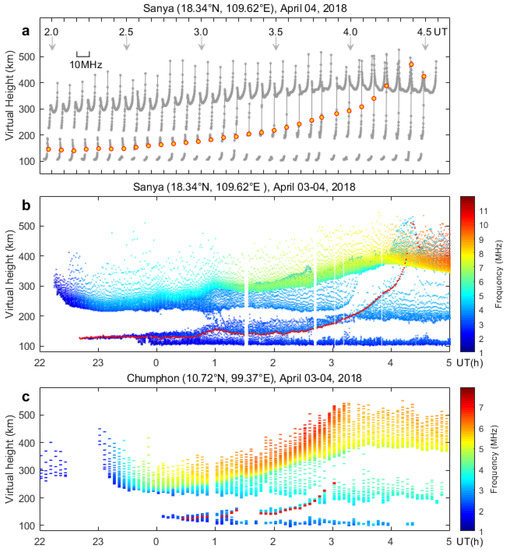
Figure 2.
(a). Sequence of ordinary wave traces by the Sanya PDI with 5 min resolution during 0200–0430 UT (0918–1148 LT) on 4 April 2018. The red circle indicates the virtual height of the ascending ion layer. The ionograms obtained at 0200, 0230, 0300, 0330, 0400, and 0430 UT are marked by arrows. (b,c) Summary plots of manually scaled ordinary wave traces from the ionograms observed by the Sanya and Chumphon ionosondes during the period 2200 UT, 3 April—0500 UT, 4 April 2018. The plasma frequencies are color-coded as functions of virtual height and time. Note that if multiple frequencies correspond to the same virtual height, there will be an overlap between the higher and lower frequency dots (the lower frequency dots will be covered by the higher frequency dots). The overlap is obvious at larger virtual heights, where the plasma frequency shows abrupt changes with virtual height. The red dots superimposed in the panels indicate the virtual height of the ascending ion layer.
The ascending ion layer at low latitude Sanya, from the upper E to F region, is similar to the rising structure observed by the Jicamarca radar at the magnetic equator [25,26]. It was suggested that the equatorial rising structure was due to the fringe electric fields associated with the initial development of equatorial spread-F (ESF). This, however, cannot explain the present observations because the ascending ion layer was observed during daytime, when generally no ESF was generated. Based on the Arecibo ISR observations, high Es layers with downward movement were frequently observed in daytime and suggested to be controlled by semi-diurnal tides [8]. Recent simulations supported that the day to day variations in the daytime high Es layer were generated mainly by the vertical shears of zonal winds driven by the semi-diurnal tides [27]. In the present study, the high Es layer (ascending ion layer) initially appeared at 0558 LT at the virtual (true) height of 125 km (115–120 km) over Sanya. As pointed out by Haldoupis [5], at the altitudes below 125 km, the zonal wind shear mechanism is dominant on the Es layer formation. Therefore, the generation of the high Es layer observed over Sanya was most likely driven by the zonal wind shear. However, the uplift of the ion layer in later hours was unlikely to be controlled by the tidal wind, because the zonal wind shear node driven by tidal winds normally shows a downward propagation phase [8,27,28].
Based on the feature that the uplift of the ion layer was in a pattern similar to that of the F region, we surmise that the uplift could be mainly driven by a background electric field. In this regard, the measurements by an equatorial ionosonde may provide evidence to support this argument. Fortunately, the ionosonde at Chumphon, an equatorial station in this longitude sector, recorded continuous ionograms on that day (part of the ionograms are shown in Figure S3 in data repository). Figure 2c displays the summary plot of manually scaled ordinary wave trace with a time resolution of 5 min at Chumphon. Two interesting features can be noted. One is that an ascending ion layer was also observed at the magnetic equator around the same period, which started from ~0200 UT, connected to the F region bottomside at ~0300 UT, and then disappeared in the F2 layer trace. This result indicates that the ascending of the ion layer occurred simultaneously over a large latitude region from the magnetic equator to the low latitude (>12° dip latitude) far away from the magnetic equator. The other is that at the magnetic equator, the uplift of the ion layer was also in a pattern similar to the vertical drift of the F region, providing a solid evidence for the driving of the ion layer uplift by the background eastward electric field.
Figure 3 shows the true height variations of the ascending ion layer and the F layer peak height (hmF2) at Sanya and Chumphon during 0000–0600 UT on 4 April 2018. Note that for the ion layer, only when its trace connected with the F layer trace could the true height be retrieved by the NHPC algorithm. It can be seen from Figure 3 that over Chumphon, the F layer peak height (hmF2) increased roughly from 263 km to 312 km during 0215–0255 UT, showing an average upward drifting velocity of ~20 m/s. During 0240–0250 UT, the ion layer height varied from 140 km to 150 km, indicating an average ascending velocity of ~17 m/s. Over Sanya, the vertical drifts of hmF2 and the ion layer during 0310–0415 UT were estimated to be ~10 m/s and ~8 m/s, respectively. It is evident that the ion layer and F region show similar upward drift at both equatorial and low latitudes, which was suggested to be driven by daytime background eastward electric field. Furthermore, there are two notable differences. One is that the ascending velocity of the ion layer is slightly lower than that of hmF2. This could be attributed to higher ion-neutral collision frequency at a lower height, which reduces the vertical drift velocities of the ion layer in the upper E region to the lower F region [14]. The other is that the upward drifts of hmF2 and the ion layer at low latitude are approximately half of those at the magnetic equator. This may be due to the fact that the vertical drifts driven by electric fields (E × B/B2) are strongly dependent on latitude. Due to the decrease in electric field strength and the increase in magnetic field inclination with latitude, the vertical drift velocity decreases correspondingly in the poleward direction [16].
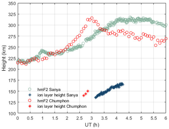
Figure 3.
The F layer peak height (hmF2) and the true height of ascending ion layer retrieved from the manually scaled ionograms by the Sanya and Chumphon ionosondes during 0000–0600 UT on 4 April 2018.
Lee et al. [19] reported an ascending thin layer event during the morning hour in the equatorial F region at Jicamarca. The thin layer, with topside and bottomside scale heights of 2.8–5.0 and 1.2–2.4 km, was lifted upward from the F1 layer to the F2 layer with a velocity of 15.5 m/s. The ascending velocity of the thin layer observed at Chumphon is similar to that at Jicamarca. The Jicamarca ascending thin layer case provided evidence for the vertical transport of metallic ions in the equatorial F region. Santos et al. [12] reported another case of an ascending thin layer at São Luís in the American sector. The thin layer ascended from 150 km to 420 km (both virtual height) in 1.5 h. Our results on ascending velocity of ion layer at Chumphon is in line with those from the American equatorial region (Jicamarca and São Luís). All the ascending layer events occurred in morning hours in the spring equinox season (October in Southern American and April in East Asia). Moreover, the present observations showed the clear ascending process of the thin layer from the E region to the F region. However, due to the low signal strength of Chumphon ionosonde data, the uplift of the thin ion layer in the F2 region could not be clearly observed.
By using the OGO 6 satellite measurements, Hanson and Sanatani [14] have reported the presence of metallic ions above the F2 layer peak. They surmised that the E × B drift driven by the equatorial dynamo electric field was the active agent lifting the E region metallic ions to the F region topside around the magnetic equator. The metallic ions in the equatorial F region topside could then be transported to higher latitudes through the effect of gravity and diffusion (i.e., the equatorial fountain effect). This process was simulated by Carter and Forbes [16]. The present observations at Chumphon provide direct evidence for the upward moving of the ion layer from the equatorial E region to the F region. Furthermore, the simultaneous observations at low latitude Sanya show that in addition to the equatorial fountain effect, the ion layers could be lifted directly from the local E to F region at the latitudes far away from the magnetic equator, providing another source for the F region metallic ions. This result offers another possibility for the explanation of a metallic ion source responsible for the high altitude metallic layers observed at off-equatorial latitudes. In this regard, one important question is how often this type of ascending ion layer occurs at low latitudes. Based on the daily summary plots (see, for example, Figure 2b) obtained at Sanya, a statistical analysis was performed. If an ascending ion layer was seen from the summary plot, we then manually checked each ionogram during the interval of the ascending ion layer and obtained its onset time and duration. Note that at Chumphon, some ionograms are not good enough to identify the ascending ion layer, and thus, the statistical feature cannot be well obtained.
Figure 4 displays the statistical results of ascending ion layer occurrence over Sanya during the periods December 2017–June 2018 and April 2019–June 2020. Out of a total of 511 days with data, 38 ascending ion layer events were observed. As shown in Figure 4a, the occurrence rate of the ascending ion layer shows two peaks in spring (March and April) and quasi-autumn months (August, September). No ascending ion layer event was observed in January and December. Figure 4b,d show that all the ion layer events started to ascend in the morning hours and ended before 1300 LT, mostly with durations of 0.5–2.5 h. The results show that the ascending ion layer is entirely a morning phenomenon. These results are also in line with the descending upper Es layer trace observed over Arecibo, which mostly descended from 130 km starting at 9–12LT [8]. On the days with an ascending ion layer, both high and low Es layers appeared, but it was always the high type Es layer that moved upward to the F region (similar to that shown in Figure 2).
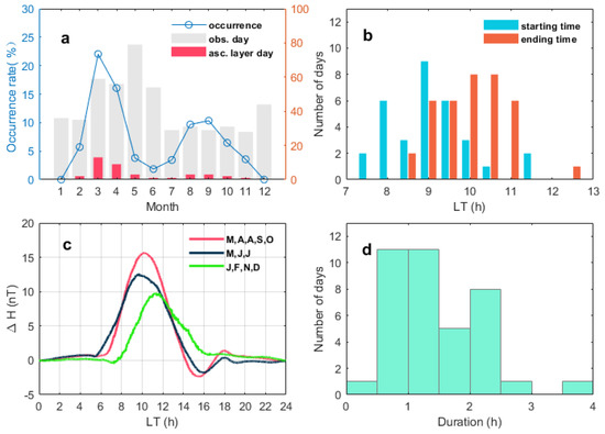
Figure 4.
(a). The occurrence rate of the ascending ion layer versus month during December 2017–June 2018 and April 2019–June 2020. The gray and red bars indicate the numbers of days with data and with an ascending ion layer, respectively. (b). The distributions of starting time and ending time for the ascending ion layer in local time. (c). The variation in the average ∆H components derived from the measurements at magnetic equator Da Lat and low latitude Sanya versus local time. The red, black, and green lines indicate the results in March, April, August, September, and October (M, A, A, S, O months), May, June, and July (M, J, J months), January, February, November, and December (J, F, N, D months), corresponding to the relatively high, moderate, and low occurrence months of ascending ion layers in the panel (a), respectively. (d). The distributions of duration of the ascending ion layer.
Next, we consider what may control the seasonal variation of the ascending ion layer. As presented above, the background eastward electric field is suggested to be the most likely driving mechanism for the uplift of the thin layer simultaneously observed at Chumphon and Sanya. However, for the statistical results over Sanya, we cannot rule out the possibility of a neutral wind effect. Theoretical simulations have shown that neutral wind can also transport metallic ions upward at low latitudes away from the magnetic equator and at the polar region [27,29]. For example, Andoh et al. [27] reported two cases of an ascending metallic ion layer due to the Lorentz force driven by the eastward wind over Arecibo.
To investigate if there is any statistical relationship between the seasonal variations of the ascending ion layer and of the background eastward electric field, we employed the magnetometer data at the equatorial station Da Lat (11.9°N, 108.5°E, dip lat. 5.3°N) and low latitude station Sanya to calculate the difference in the magnetic field horizontal component (∆H). In previous studies, it was proven that the ∆H provides a direct measure of the daytime electrojet current and, in turn, the magnitude of the vertical E × B drift velocity in the F region ionosphere [30]. A positive ∆H indicates an eastward electric field. During the periods December 2017–June 2018 and April 2019–June 2020, there were a total of 416 days with simultaneous ∆H and ionosonde data. Figure 4c shows the variation in average ∆H in high, moderate, and low occurrence months for the ascending ion layer. It is evident that in the months when the occurrence rate of the ascending ion layer is high (M, A, A, S, O months), the background eastward electric field (characterized by the ∆H) is the strongest. In the J, F, N, D months when the occurrence rate of the ascending ion layer is low, the background eastward electric field is the weakest. On the other hand, it is found that the average ∆H on the days with (without) ascending ion layer, the background eastward electric field in the morning hours is relatively strong (weak) (figures in Supplementary Materials). The close correlation between the strength of the background eastward electric field and the occurrence of the ascending ion layer suggests that a stronger background eastward electric field is more likely to drive the uplift of the ion layer.
Another interesting aspect is that the seasonal variation of the ascending ion layer observed at Sanya is quite consistent with that of the Mg+ intensity reported previously. Based on the ESRO TD1 satellite observations, Gérard [31] investigated the annual variation of Mg+ intensity during sunset hours at the F region topside in 125–160°E. Their results showed two occurrence peaks of Mg+ in the equinoctial month, with the major and minor peaks in spring and autumn, respectively. This good agreement suggests that the uplifted ion layer from the local E to F regions at low latitudes could contribute significantly to the F region metallic ions observed by satellite-based in situ payloads.
It is worth noting that though the ascending thin layer is likely to be driven by the background electric field, the reason why the ions could be concentrated to maintain a thin layer during their ascending is unknown. Further investigation with new observations and simulations is required. In the observation aspect, lidar observation can provide fine temporal variation in metallic species at given locations [27,28,29], which would shed new light on the study of the ascending high Es layer. However, this is beyond the scope of this study and will be addressed in future studies.
4. Conclusions
Using high temporal resolution ionogram measurements at Chumphon (5 min cadence) and Sanya (1 min/2 min cadence), ascending layers from the upper E region to the F region were simultaneously observed at equatorial and low latitudes for the first time. The equatorial (low latitude) ion layer ascended with a mean velocity of 17 m/s (8 m/s), in a pattern similar to that of the F region peak height. The background eastward electric field was suggested to play an important role on the uplift of the ion layer. Further statistical results showed that at low latitude Sanya, the ascending ion layer from the local E to F region was not a rare phenomenon, with two occurrence peaks up to 22% and 10% in the spring and quasi-autumn months, respectively. All the ascending ion layers occurred in the morning hours. A good agreement between the seasonal variations in the ascending ion layer in morning hours and in Mg+ intensity at the F region during sunset hours was found. Since the Es layer is widely accepted to be composed of metallic ions, the results suggest that in addition to the equatorial fountain effect, the metallic ions in the ascending ion layers could be lifted directly from the local E to F region at the latitudes far away from magnetic equator. These uplifted ions from the local E region could contribute significantly to the high altitude metallic ions and offer another possibility for the explanation of the metallic ion source responsible for the high altitude metallic atom layers observed at off-equatorial latitudes. It is expected that fast ionogram observations, together with the measurements by a collocated lidar, which is capable of detecting the metallic species with high sensitivity, will help to reveal the formation of some unexpected high altitude metallic layers.
Supplementary Materials
The following supporting information can be downloaded at: https://doi.org/10.12197/2022GA006 accessed on 26 October 2022, Figure S1, An animation of ionograms between 2200UT, 3 April 2018—0500UT, 4 April 2018 at Sanya; Figure S2, A sequence of ionograms on 4 April 2018 at Fuke; Figure S3, A sequence of ionograms on 4 April 2018 at Chumphon.
Author Contributions
Conceptualization, G.L.; methodology, G.L. and B.N.; software, L.H.; validation, X.Z. and H.X.; formal analysis, L.H.; investigation, L.H. and G.L.; data curation, W.S., Z.Z., J.L., Z.H. and T.Y.; writing—original draft preparation, L.H.; writing—review and editing, G.L., Z.D. and Z.Z.; visualization, L.H.; supervision, G.L. and B.N. All authors have read and agreed to the published version of the manuscript.
Funding
This work was supported by the Project of Stable Support for Youth Team in Basic Research Field, CAS (YSBR-018), the National Natural Science Foundation of China (42074190, 42020104002, 41727803 and 41904141), and the Informatization Plan of Chinese Academy of Sciences (CAS-WX2021SF-0303, CAS-WX2021PY-0101).
Data Availability Statement
The Sanya ionosonde and magnetometer data were provided by Beijing National Observatory of Space Environment, Institute of Geology and Geophysics, CAS through the Geophysics center, National Earth System Science Data Center (http://wdc.geophys.ac.cn/, accessed on 21 March 2021). The Fuke ionosonde data were downloaded from the data center of Chinese Meridian Project (https://data.meridianproject.ac.cn/, accessed on 16 March 2022). The Chumphon ionosonde data were downloaded at the SEALION website (https://aer-nc-web.nict.go.jp/sealion/, accessed on 30 October 2021). The Da Lat magnetometer data were downloaded from the Bureau Central de Magnetisme Terrestre (http://www.bcmt.fr/, accessed on 26 January 2022) The Kp index was downloaded from WDC Geomagnetism, Kyoto (http://wdc.kugi.kyoto-u.ac.jp/, accessed on 3 March 2021). All the data used in this study are also archived at the WDC for Geophysics, Beijing (https://doi.org/10.12197/2022GA006, accessed on 25 October 2022).
Conflicts of Interest
The authors declare no conflict of interest.
References
- Li, G.; Ning, B.; Abdu, M.A.; Wan, W.; Hu, L. Precursor signatures and evolution of post-sunset equatorial spread-F observed over Sanya. J. Geophys. Res. 2012, 117, A08321. [Google Scholar] [CrossRef]
- Sun, W.; Ning, B.; Hu, L.; Yue, X.; Zhao, X.; Lan, J.; Zhu, Z.; Huang, Z.; Wu, Z. The evolution of complex Es observed by multi instruments over low-latitude China. J. Geophys. Res. Space Phys. 2020, 125, e2019JA027656. [Google Scholar] [CrossRef]
- Sarudin, I.; Hamid, N.S.A.; Abdullah, M.; Buhari, S.M.; Shiokawa, K.; Otsuka, Y.; Hozumi, K.; Jamjareegulgarn, P. Influence of zonal wind velocity variation on equatorial plasma bubble occurrences over Southeast Asia. J. Geophys. Res. Space Phys. 2021, 126, e2020JA028994. [Google Scholar] [CrossRef]
- Abadi, P.; Ahmad, U.A.; Otsuka, Y.; Jamjareegulgarn, P.; Martiningrum, D.R.; Faturahman, A.; Perwitasari, S.; Saputra, R.E.; Septiawan, R.R. Modeling Post-Sunset Equatorial Spread-F Occurrence as a Function of Evening Upward Plasma Drift Using Logistic Regression, Deduced from Ionosondes in Southeast Asia. Remote Sens. 2022, 14, 1896. [Google Scholar] [CrossRef]
- Haldoupis, C. “A Tutorial Review on Sporadic E Layers,” Aeronomy of the Earth’s Atmosphere and Ionosphere, IAGA Special Sopron Book Series, 2nd ed.; Springer: Berlin/Heidelberg, Germany, 2011; pp. 381–394. [Google Scholar]
- Smith, L.G. Rocket Observations of Sporadic E and Related Features of the E Region. Radio Sci. 1966, 1, 178–186. [Google Scholar] [CrossRef]
- Young, J.M.; Johnson, C.Y.; Holmes, J.C. Positive ion composition of a temperate-latitude sporadic E layer as observed during a rocket flight. J. Geophys. Res. 1967, 72, 1473–1479. [Google Scholar] [CrossRef]
- Christakis, N.; Haldoupis, C.; Zhou, Q.; Meek, C. Seasonal variability and descent of mid-latitude sporadic E layers at Arecibo. Ann. Geophys. 2009, 27, 923–931. [Google Scholar] [CrossRef]
- Haldoupis, C.; Meek, C.; Christakis, N.; Pancheva, D.; Bourdillon, A. Ionogram height–time–intensity observations of descending sporadic E layers at mid-latitude. J. Atmos. Sol.-Terr. Phys. 2006, 68, 539–557. [Google Scholar] [CrossRef]
- Lee, C.-C.; Liu, J.-Y.; Pan, C.-J.; Hsu, H.-H. The intermediate layers and associated tidal motions observed by a digisonde in the equatorial anomaly region. Ann. Geophys. 2003, 21, 1039–1045. [Google Scholar] [CrossRef]
- Oikonomou, C.; Haralambous, H.; Leontiou, T.; Tsagouri, I.; Buresova, D.; Mošna, Z. Intermediate descending layer and sporadic E tidelike variability observed over three mid-latitude ionospheric stations. Adv. Space Res. 2022, 69, 96–110. [Google Scholar] [CrossRef]
- dos Santos, Â.M.; Batista, I.S.; Abdu, M.A.; Sobral, J.H.A.; de Souza, J.R.; Brum, C.G.M. Climatology of intermediate descending layers (or 150 km echoes) over the equatorial and low-latitude regions of Brazil during the deep solar minimum of 2009. Ann. Geophys. 2019, 37, 1005–1024. [Google Scholar] [CrossRef]
- Mathews, J.D. Sporadic E: Current views and recent progress. J. Atmos. Sol.-Terr. Phys. 1998, 60, 413–435. [Google Scholar] [CrossRef]
- Hanson, W.B.; Sanatani, S. Meteoric Ions above the F2 Peak. J. Geophys. Res. Space Phys. 1970, 75, 5503–5509. [Google Scholar] [CrossRef]
- Cai, X.; Yuan, T.; Eccles, J.V.; Pedatella, N.M.; Xi, X.; Ban, C.; Liu, A.Z. A numerical investigation on the variation of sodium ion and observed thermospheric sodium layer at Cerro Pachón, Chile during equinox. J. Geophys. Res. Space Phys. 2019, 124, 10395–10414. [Google Scholar] [CrossRef]
- Carter, L.N.; Forbes, J.M. Global transport and localized layering of metallic ions. Ann. Geophys. 1999, 17, 190–209. [Google Scholar] [CrossRef]
- Chu, X.; Yu, Z. Formation mechanisms of neutral Fe layers in the thermosphere at Antarctica studied with a thermosphere-ionosphere Fe/Fe+ (TIFe) model. J. Geophys. Res. Space Phys. 2017, 122, 6812–6848. [Google Scholar] [CrossRef]
- Huba, J.D.; Krall, J.; Drob, D. Global ionospheric metallic ion transport with SAMI3. Geophys. Res. Lett. 2019, 46, 7937–7944. [Google Scholar] [CrossRef]
- Lee, C.-C.; Su, S.-Y.; Reinisch, B.W. An upward moving thin layer in the equatorial F region observed by a digisonde. J. Geophys. Res. 2008, 113, A10302. [Google Scholar] [CrossRef]
- Lan, J.; Ning, B.; Li, G.; Zhu, Z.; Hu, L.; Sun, W. Observation of short-period ionospheric disturbances using a portable digital ionosonde at Sanya. Radio Sci. 2018, 53, 1521–1532. [Google Scholar] [CrossRef]
- Saito, S.; Maruyama, T. Ionospheric height variations observed by ionosondes along magnetic meridian and plasma bubble onsets. Ann. Geophys. 2006, 24, 2991–2996. [Google Scholar] [CrossRef]
- Nozaki, K. FMCW lonosonde for the SEALION project. J. Natl. Inst. Inf. Commun. Technol. 2009, 56, 287–298. [Google Scholar]
- Khmyrov, G.M.; Galkin, I.A.; Kozlov, A.V.; Reinisch, B.W.; McElroy, J.; Dozois, C. Exploring digisonde ionogram data with SAO-X and DIDBase. AIP Conf. Proc. 2008, 974, 175–185. [Google Scholar] [CrossRef]
- Huang, X.; Reinisch, B.W. Vertical electron content from ionograms in real time. Radio Sci. 2001, 36, 335–342. [Google Scholar] [CrossRef]
- Woodman, R.F.; Chau, J.L. Equatorial quasiperiodic echoes from field-aligned irregularities observed over Jicamarca. Geophys. Res. Lett. 2001, 28, 207–209. [Google Scholar] [CrossRef]
- Kherani, E.A.; Raghavarao, R.; Sekar, R. Equatorial rising structure in nighttime upper E-region: A manifestation of electrodynamical coupling of spread F. J. Atmos. Sol.-Terr. Phys. 2002, 64, 1505–1510. [Google Scholar] [CrossRef]
- Andoh, S.; Saito, A.; Shinagawa, H. Numerical simulations on day-to-day variations of low-latitude Es layers at Arecibo. Geophys. Res. Lett. 2022, 49, e2021GL097473. [Google Scholar] [CrossRef]
- Chu, X.; Chen, Y.; Cullens, C.Y.; Yu, Z.; Xu, Z.; Zhang, S.-R.; Huang, W.; Jandreau, J.; Immel, T.J.; Richmond, A.D. Mid-latitude thermosphere ionosphere Na (TINa) layers observed with high-sensitivity Na Doppler lidar over Boulder (40.13°N, 105.24°W). Geophys. Res. Lett. 2021, 48, e2021GL093729. [Google Scholar] [CrossRef]
- Chu, X.; Nishimura, Y.; Xu, Z.; Yu, Z.; Plane, J.M.C.; Gardner, C.S.; Ogawa, Y. First simultaneous lidar observations of thermosphere ionosphere Fe and Na (TIFe and TINa) layers at McMurdo (77.84°S, 166.67°E), Antarctica with concurrent measurements of aurora activity, enhanced ionization layers, and converging electric field. Geophys. Res. Lett. 2020, 47, e2020GL090181. [Google Scholar] [CrossRef]
- Anderson, D.; Anghel, A.; Yumoto, K.; Ishitsuka, M.; Kudeki, E. Estimating daytime vertical ExB drift velocities in the equatorial F-region using ground-based magnetometer observations. Geophys. Res. Lett. 2002, 29, 37-1–37-4. [Google Scholar] [CrossRef]
- Gérard, J.-C. Satellite measurements of high-altitude twilight Mg+ Emission. J. Geophys. Res. Space Phys. 1976, 81, 83–87. [Google Scholar] [CrossRef]
Publisher’s Note: MDPI stays neutral with regard to jurisdictional claims in published maps and institutional affiliations. |
© 2022 by the authors. Licensee MDPI, Basel, Switzerland. This article is an open access article distributed under the terms and conditions of the Creative Commons Attribution (CC BY) license (https://creativecommons.org/licenses/by/4.0/).