Abstract
Toxic metals have attracted great concern worldwide due to their toxicity and slow decomposition. Although metal concentrations can be accurately obtained with chemical methods, it is difficult to map metal distributions on a large scale due to their inherently low efficiency and high cost. Moreover, chemical analysis methods easily lead to secondary contamination. To address these issues, 110 topsoil samples were collected using a soil sampler, and positions for each sample were surveyed using a global navigation satellite system (GNSS) receiver from a coal mine in northern China. Then, the metal contents were surveyed in a laboratory via a portable X-ray fluorescence spectroscopy (XRF) device, and GaoFen-5 (GF-5) satellite hyperspectral images were used to retrieve the spectra of the soil samples. Furthermore, a Savitzky–Golay (SG) filter and continuous wavelet transform (CWT) were selected to smooth and enhance the soil reflectance. Competitive adaptive reweighted sampling (CARS) and Boruta algorithms were utilized to identify the feature bands. The optimum two-stage method, consisting of the random forest (RF) and ordinary kriging (OK) methods, was used to infer the metal concentrations. The following outcomes were achieved. Firstly, both zinc (Zn) (68.07 mg/kg) and nickel (Ni) (26.61 mg/kg) surpassed the regional background value (Zn: 48.60 mg/kg, Ni: 19.5 mg/kg). Secondly, the optimum model of RF, combined with the OK (RFOK) method, with a relatively higher coefficient of determination (R2) (R2 = 0.60 for Zn, R2 = 0.30 for Ni), a lower root-mean-square error (RMSE) (RMSE = 12.45 mg/kg for Zn, RMSE = 3.97 mg/kg for Ni), and a lower mean absolute error (MAE) (MAE = 9.47 mg/kg for Zn, MAE = 3.31mg/kg for Ni), outperformed the other four models, including the RF, OK, inverse distance weighted (IDW) method, and the optimum model of RF combined with IDW (RFIDW) method in estimating soil Zn and Ni contents, respectively. Thirdly, the distribution of soil Zn and Ni concentrations obtained from the best-predicted method and the GF-5 satellite hyperspectral images was in line with the actual conditions. This scheme proves that satellite hyperspectral images can be used to directly estimate metal distributions, and the present study provides a scientific base for mapping heavy metal spatial distribution on a relatively large scale.
Keywords:
heavy metals; random forest; interpolation method; remote sensing inversion; XRF; GaoFen-5 1. Introduction
Soil, an essential part of the terrestrial ecosystem and one of the valuable natural resources for agriculture, is an important base for socioeconomic development and human survival [1]. However, soils have suffered serious toxic metal contamination throughout the world, especially in developing countries under the background of rapid urbanization and industrialization [2]. The major sources of poisonous metals are various smelting and mining activities, as well as the deposition of particulates from mining operations, pesticide utilization, and industrial production [3]. China, the largest coal consumer and producer in the world, is undergoing rapid socioeconomic development [4]. Nevertheless, coal mining activities may impose negative effects on ecosystems and the natural environment, especially on cropland near coal mines [5]. Toxic metals in soils exhibit significantly harm to crops and humans due to to their carcinogenic properties, toxicity, cumulative effects, and non-degradability [6]. What is worse, toxic metals impose negative effects on human health and lead to soil degradation via accumulation in the food chain [7]. For example, gastrointestinal distress, such as abdominal pain, nausea, irritation of the respiratory system, and vomiting, can be generated by inhaling excessive zinc (Zn) [8]. More seriously, fertility and cholesterol balance may be impacted by long-term high-dose exposure to Zn [9]. Additionally, studies indicate that chronic exposure to nickel (Ni) may increase the risk of cancer [10]. Hence, investigating toxic metal contaminations in coal mining areas is strongly desired because the outcomes can be used to identify polluted areas, provide land reclamation strategies, select soil remediation schemes, and propose effective public health prevention measures.
The rapid and accurate measurement of heavy metal concentrations is the prerequisite to obtaining its spatial distribution. Traditionally, ground-level soil sampling and laboratory surveying, including inductively coupled plasma (ICP), X-ray fluorescence spectroscopy (XRF), and atomic absorption spectrometry (AAS), [11,12,13,14,15], have commonly been adopted to measure toxic metal contents in soil. Moreover, the spatial distribution of heavy metals can also be obtained via geostatistical methods, which can infer heavy metal concentrations in unsampled locations [16]. Nevertheless, traditional approaches are labor and time-consuming and may lead to secondary contamination due to extra chemicals used in the laboratory process. Moreover, the above methods, showing low efficiency, have difficulty meeting the need for the rapid investigation of heavy metal distributions at a relatively large scale [17]. Additionally, geostatistics mainly depends on the assumptions of spatial autocorrelation, whereas the actual heavy metals may demonstrate significant spatial heterogeneity due to the diverse chemical and physical properties of the soils and the environment [18].
Recently, hyperspectral remotely sensed technology (RST) has been used to rapidly and accurately estimate soil heavy metal concentrations in large areas [19]. Currently, estimating heavy metal contents with RST can be divided into two types: one uses multi-spectral data, combining auxiliary variables such as the chemical and physical properties of soils, topography elements, and environmental factors to infer the distribution of heavy metals [20,21,22,23,24]; the other type takes advantage of hyperspectral RST to fit a quantitative model between soil heavy metal concentrations and the spectra of soil samples, inferring the metal distributions [25,26,27]. However, the capacity and sensitivity of multi-spectral RST are relatively inadequate. In addition, auxiliary variables for inferring soil heavy metal contents with multi-spectral RST vary according to sampling locations and the lack of universality [28]. Hyperspectral RST can be used to infer heavy metal concentrations because metals have a stronger direct response to organic matter and clay signals when the metals are attached to exchange sites.
Although hyperspectral RST showed convenience and feasibility for predicting heavy metal concentrations, to some extent, some uncertainties and deficiencies still exist [29]. Hyperspectral images can be collected by airborne and space-borne platforms [30]. However, the spectral resolution of some sensors, with a low signal-to-noise ratio (SNR), is coarse. For instance, Hyperion, the short-wave infrared (SWIR) spectral channel with a low SNR, was decommissioned in 2017. Compact High-Resolution Imaging Spectrometer (CHRIS) with the visible-to-near infrared (VNIR) spectral range (415–1050 nm) can hardly be used to inverse heavy metals because the spectral cover is not large enough [31]. Fortunately, the SWIR Advanced Hyperspectral Imager (AHSI), covering 330 bands to reflect solar reflection during 350–2500 nm, with a narrow swath width of approximately 60 km, one of the main payloads onboard the GaoFen-5 (GF-5) satellite, supplies a probability for retrieving heavy metal contents from a relatively large region [32]. The spectral resolution for VNIR and the SWIR is about 5 nm and about 10 nm, respectively, and the maximum SNR is 500 [33]. Hence, the feasibility of utilizing GF-5 satellite data to retrieve toxic metal contents requires further evaluation.
For the soil heavy metals prediction model, a series of data-driven methods, including the extreme learning machine (ELM), partial least squares regression (PLSR), support vector machine (SVM), random forest (RF), and back propagation neural networks (BPNN) methods, have recently been widely used [34,35]. Although the issue of linear fitting can be solved by machine learning methods, it shows some drawbacks regarding model robustness and efficiency, as well the tendency to overfit. Furthermore, the spatial distribution of toxic metals was affected by both physical factors—topography factors, wind orientation, and precipitation, and by anthropogenic activities—air pollution emissions, contamination sources, and industrial production [36]. The use of machine learning methods, such as RF, often exhibit difficulty in reflecting the residuals caused by a random process and other factors, leading to the necessity of the precision inherent in the data-driven methods in estimating soil heavy metal contents, which require further improvement [37]. Previous studies have confirmed that using multi-spectral data, as well as auxiliary variables via a machine learning model combined with geological statistical models, can enhance the precision in predicting soil heavy metal concentrations [38]. However, the possibility and reliability of using hyperspectral images and a machine learning model combined with a geological statistical model to predict soil heavy metal contents have not been assessed previously.
Therefore, the purpose of this study is (1) to verify the feasibility of using GF-5 image and RF, combined with geological statistical models, including ordinary kriging (OK) and inverse distance weighting (IDW), in predicting Zn and Ni concentrations at an opencast coal mine; (2) to obtain the optimal inversion model for Zn and Ni; and (3) to clarify the spatial distribution features of Zn and Ni in the study area.
2. Materials and Methods
Figure 1 is a workflow that shows all methods and describes the main steps followed in the study. The flow chart is composed of four parts: data preparation, spectra pretreatment and feature selection, model calibration and validation, and mapping heavy metal concentrations.

Figure 1.
The flowchart of this study.
First, the remote sensing images of GF-5 are preprocessed, which consists of radiometric calibration, atmospheric correction, and mixed pixel decomposition. It also covers soil sample preprocessing and heavy metal contents determination.
The second part is spectral data processing, mainly including Savitzky–Golay (SG) smoothing and continuous wavelet transform (CWT) of GF-5 image data, as well as spectral reflectance extraction using ArcGIS 10.0 for constructing the spectral database. The spectral reflectance of GF-5 and soil heavy metal contents were defined as independent variables and dependent variables, respectively, then the adaptive reweighted competitive sampling (CARS) method and Boruta algorithms were used to select the characteristic bands.
Third, RF models were fitted based on independent variables and dependent variables to determine the optimum model for heavy metal concentrations. The predicted heavy metal contents obtained from the optimum model deduced the actual heavy metal contents surveyed in the lab to determine the residual. Then residual was interpolated using OK and IDW to obtain residual distribution maps.
Fourth, the final heavy metal contents map was generated by overlaying the residual distribution maps and metal distribution maps obtained from the optimum model.
2.1. Study Area
The research site is adjacent to an open-pit mine located in the Ordos Plateau, Inner Mongolian, China (Figure 2). The topography is generally flat in the east and high in the west, with an altitude range of 850 m to 2149 m. The typical annual precipitation and temperature range from 170 mm to 450 mm and 5.3 °C to 8.7 °C, respectively. The coal resources of the Ordos Plateau are rich [39]. Moreover, the coal industry is very important for the economic growth of the Ordos. Nevertheless, mining activities generate obvious passive influences on the natural environment. Recently, heavy metal pollution around the coal mine, especially in the nearby cropland, has aroused wide concerns.
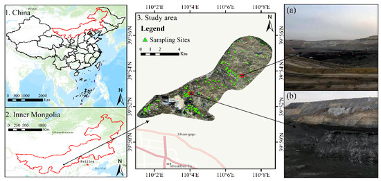
Figure 2.
The map of soil sampling sites; (a,b) show photos of the areas of the sampling field.
2.2. Soil Sample Collection and Measurement
A total of 110 soil samples, with a depth of about 20 cm, were collected in February 2020 according to the procedure listed in the FOREGS Geochemical Mapping Field Manual [40]. The soil sample sites were distributed in the farmlands of the coal mine areas to eliminate human influences and to ensure a reasonable distribution, as much as possible. Additionally, to obtain the precise geographic location of each soil sample, the global navigation satellite system (GNSS) with the real-time kinematic (RTK) method and the Continuous Operating Reference Station (CORS) signals were used to determine each sampling site’s position. The China Geodetic Coordinate System 2000 (CGCS2000) was defined as the coordinate system of the current project.
In the laboratory, the samples were first air dried. Then, the samples were ground using grinding rods, and other foreign matter was removed. Third, all soil samples were placed into an oven until dry, without changing the weight. Fourth, the samples were sieved using a 0.7 mm nylon aperture sieve and put into clean polyethylene bags for analysis [8].
For quality control and quality assurance (QC/QA), the contents of toxic metals were surveyed using a SPECTRO xSORT X-ray device. The SPECTRO xSORT had been calibrated using the geochemical reference standards and the GSS series from the GSD series (China Institute of Geophysical and Geochemical Survey, Langfang, China) to ensure that the relative standard deviation was in the range of 3% to 5% [9].
2.3. Hyperspectral Remotely Sensed Data Collection and Pretreatment
2.3.1. Acquisition and Processing of GF-5 Data
The AHSI sensor is included in the GF-5 and can be obtained at https://www.cheosgrid.org.cn/index.htm (accessed on 5 April 2020). The GF-5 image, with a spatial resolution of 30 m and a sweep width of 60 km, covers 330 wavelength bands, including the VNIR and SWIR bands regions from 390 to 2513 nm. Specifically, the spectral resolutions of the VNIR and SWIR bands were 4.28 nm and 8.42 nm, respectively, and the SNR in the VNIR and SWIR regions was about 700 and 500, respectively. Several methods, including radiometric calibration, atmospheric correction, and orthorectification, were adopted to process the GF-5 image. The spectral data of the sample sites can be extracted via ArcGIS 10.0, and detailed information in terms of GF-5 data processing was exclusively stated in the published paper [41]. Therefore, this paper does not desecribe the processes again.
2.3.2. Smoothing and Enhancing Spectra
To eliminate noise from the spectrum data, as well as to separate overlapping samples owing to the “burr” phenomenon, SG smoothing is carried out for the raw spectra. The SG method, with 21 window lengths, was selected to obtain a quadratic polynomial [42]. We have supplemented the experiment for determining the best smoothing window of SG (Figure S1). Furthermore, we have added necessary experiments for evaluating the two methods, and we found that the results for using both SG and CWT were better than those obtained using only CWT (Table S1). Thus, the SG smoothed spectra were enhanced by CWT.
The soil spectral absorption characteristics are close to the Gaussian function, so the Gaussian 4 function, with ten decomposition scales, was selected as the mother wavelet function. We used L1–L10 to represent ten decomposition scales, including 21, 22, 23, 24, 25, 26, 27, 28, 29, and 210, respectively [43].
2.4. Characteristic Bands Selection
If all hyperspectral data are directly used to fit the models, the performance of the models will be affected due to redundant data. In this paper, the CARS and Boruta algorithms are introduced to eliminate the redundancy of the hyperspectral data. CARS, which eliminates redundant and irrelevant variables while preserving informative variables, is one of the feature selection strategies employed in this study [44]. The Boruta method, which provides an intrinsic measure of each variable’s significance, known as the Z-score, was also used in this study to carry out the selection of spectral features [45]. All characteristic bands selected by the CARS and Boruta methods were tested to determine the optimal model (Figure 1). One significant point must be clearly clarified. We did not use testing data for feature selection. Only training datasets were used for feature selection in this study.
2.5. Two-Staged Schemes
The two-staged schemes, the first stage consisting of fitting the data using the random forest method to determine the optimal model, and the second stage consisting of correcting the heavy metal map obtained from the optimum model by overlaying the residual, are described as follows.
2.5.1. Random Forest (RF)
RF, one of the bagging-based integrated learning techniques, is widely used for solving classification and regression issues [46,47,48,49,50,51]. The number of decision tree classifiers (ntree), the maximum number of features (mtry), and the minimum number of samples of the leaf nodes significantly affect the model performance. In this study, a round-robin approach was used to determine the optimal mtry and ntree, and the ranges of ntree and mtry are 1 to 100 and 1 to P − 1, respectively. P is the number of independent variables, and the interval for both mtry and ntree is 1.
2.5.2. Interpolation Methods
Both the OK and the IDW models were used to spatialize the residual generated by the optimal model in the section. OK interpolation is one of the widely used kriging interpolation techniques, which assumes that every point in space has the same expected value and variance [52,53,54,55]. Meanwhile, to select the best interpolation method for estimating heavy metal contents, the IDW was also introduced to interpolate the residual, which is essentially a weighted moving average technique [56,57].
2.5.3. Overlay Methods
Firstly, we selected ten scales including 21, 22, 23, 24, 25, 26, 27, 28, 29, and 210 as wavelet scales, according to the methods used in previous studies. Secondly, we conducted feature selection using the spectra after L1-L10 wavelet transformation. Thirdly, we fitted models using the feature bands of each wavelet scale, and the precision was evaluated by R2, RMSE, and MAE. Then, the best wavelet scale with the highest precision was used in building the final model. Finally, the second stage aimed to correct the heavy metals map obtained from the optimum model by overlaying the residual map generated by the interpolation methods. The optimum model of RF, combined with OK (RFOK) and with IDW (RFIDW), was used in this study to determine the final heavy metal concentrations map [58].
2.6. Accuracy Evaluation
In this study, 70% of the samples are model calibration sets, and the other 30% are model validation sets [59]. Not all validation set samples were used in the RF model fitting. Three metrics were selected, including the coefficient of determination (R2), root-mean-square error (RMSE), and mean absolute error (MAE), to evaluate the model accuracy. The calibration sets (training dataset) were only used for model fitting and model parameter optimization. The validation sets (testing datasets) were only used for performance evaluation.
The equations corresponding to the above three metrics can be found in previous studies, so they have not been inlcuded again in this paper [60].
3. Results and Discussion
3.1. Descriptive Statistics for Heavy Metal Contents
The risk screening values for Zn and Ni are 200 mg/kg and 190 mg/kg, based on the soil environmental quality risk control standard for the soil contamination of agricultural land in China [61]. Clearly, neither Zn nor Ni’s mean value in this work surpasses the national risk screening value (Table 1). However, both Zn and Ni mean values exceed the local risk screening value. The results indicated that Zn, with a 33.14% coefficient of variation (CV), exhibits a skewed distribution, which shows that Zn has accumulated, to some extent, in the study area under the influence of long-term human activities and mining practices. However Ni, with 20.93% CV, represents a nearly normal distribution (Table 1 and Figure 3).

Table 1.
Descriptive statistics for heavy metal concentrations in the study area.
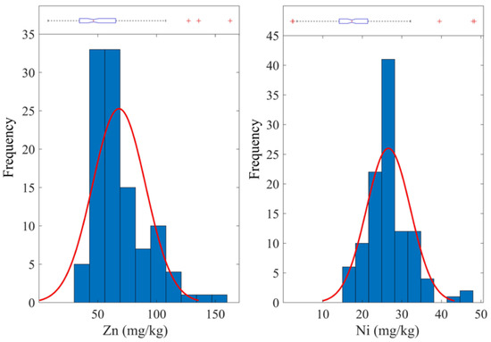
Figure 3.
Histograms and box plots of Zn and Ni concentrations (No. of samples = 110). (Note: The red curve is the fitting line; “+” denotes outliers.)
3.2. Analysis of Soil Spectral Characteristics
The original spectra for the entire 110 sample sites are shown in Figure 4a. Overall, the organic matter and iron ions lead to the soil spectral curve exhibiting an increasing trend between 350 and 1400 nm [62]. The reflection peaks caused by sensor noise are noticeable at positions between 900 and 1100 nm. Additionally, the absorption troughs at 1400, 1900, and 2200 nm are caused by the composition of water and adsorbed minerals [63]. The raw spectral reflectance was smoothed by SG smoothing, and the SG effectively eliminated noise and removed the “burr” phenomena (Figure 4b).
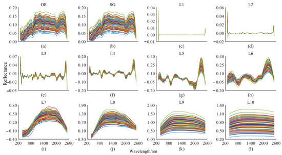
Figure 4.
Original and pretreated soil reflectance curves. (Notes: (a) OR is the original soil reflectance curve; (b) SG denotes the soil reflectance curve smoothed by SG; (c–l) L1–L10 are the reconstructed spectra using CWT at decomposition scales of 1–10).
The CWT-transformed spectra are shown in Figure 4c–l, labeled with L1–L10 for each of the 10 scales. From this figure, we can outline four general properties of wavelet spectra. The width and position of the narrow spectral features were captured in the L1–L3 spectrum, and feature identification is considerably improved using these three spectrum scales compared to the original reflectance. The L4–L6 spectrum captured properties of the continuum and retained the overall amplitude of the original reflectance spectrum. The relative strength of the features in the reflectance was preserved and enhanced in the L4–L6 spectra. In the L7–L10 spectrum, the spectral information was continuously eliminated, resulting in a flattening of the spectral curve and the loss of the majority of the spectral information [64].
In summary, it is necessary to first reduce noise from the raw spectrum data before highlighting reflection peaks and absorption valleys in the smoothed spectral data in order to gain additional spectral information. Published research has shown that the wavelet transform scale is not as broad as it could be, and as the scale increases, the spectral information gradually disappears [65,66]. As a result, the spectral curve in this study is unable to display the typical spectral features beyond the L7 scale.
3.3. Analysis of Spectral Feature Bands for Both Zn and Ni
In this work, two techniques, including the CARS and Boruta algorithms, were adopted to select the spectral feature bands. CARS uses cross-validation to choose the feature bands with the fewest root mean square errors (RMSECV), and the Boruta algorithm sieves the feature bands based on their Z-score.
The feature bands for both Zn and Ni are essentially distributed in the 300–700 nm, 1100–1400 nm, and 2300 nm ranges (Figure 5 and Figure 6). It should be noted that the distribution maps of Zn and Ni concentrations in this study were indirectly obtained from variations of SOC and clay because heavy metals have a close relationship with these types of soil.
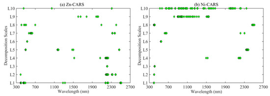
Figure 5.
The position of feature bands for Zn and Ni based on the CARS algorithm.
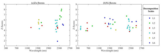
Figure 6.
The position of feature bands for Zn and Ni based on the Boruta algorithm.
For the Zn element, the feature bands were primarily located in the ranges of 400–650 nm, 1190–1520 nm, and 2340–2380 nm (Figure 5a and Figure 6a), and these results are largely in line with those of earlier investigations [67,68,69]. Zn and clay minerals exhibit a strong association, and the OH bonds in clay minerals react spectrally in this wavelength range; thus, clays have high reflection peaks around 400–600 nm, 1900 nm, and 2200 nm [70].
In contrast, Ni exhibits a significant spectral response in the region of 840–900 nm, 1330–1540 nm, and 2130–2370 nm (Figure 5b and Figure 6b). In the clay minerals, the location of these spectral feature bands is dominated by the secondary absorption peak of the Al–OH group [61,62,63,64,65,66,67,68,69,70,71,72,73]. Additionally, the organic matter exhibits a strong correlation with Ni, and the clay minerals, including kaolinite and vermiculite, also absorb Ni in this wavelength region. Clearly, spectral feature bands for both Zn and Ni demonstrate close relationships with the organic matter and clay minerals.
3.4. Prediction Model Performance Evaluation and Heavy Metal Concentrations Map Accuracy Analysis
In this study, R2, RMSE, and MAE were adopted to evaluate the RF prediction model performance, and 30% of the soil samples were defined as the validation set.
For the Zn element, the optimal RF prediction model with the highest R2 (0.4258), lowest RMSE (15.4994 mg/kg), and MAE (12.7899 mg/kg) was determined by the CARS feature selection at the L1 scale of the CWT (Figure 7a).
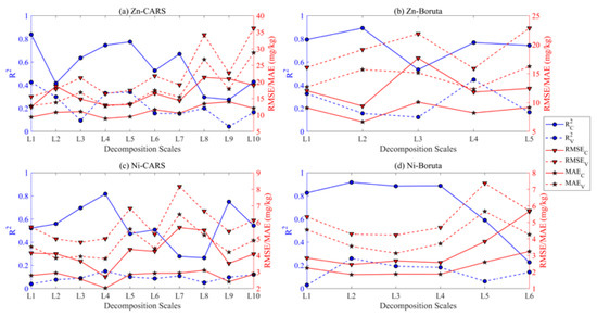
Figure 7.
Evaluating RF model performance at each decomposition scale of CWT.
For the Ni element, the best RF prediction model with the highest R2 (0.2615), lowest RMSE (4.0933 mg/kg), and MAE (3.4126 mg/kg) was determined by the Boruta feature selection at the L2 scale of the CWT (Figure 7d).
The final mapping accuracy is shown in Figure 8.
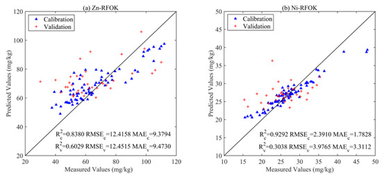
Figure 8.
Scatter plots for the optimum inversion models. (Note: (a) and (b) represent Zn and Ni, respectively.)
The heavy metal concentrations maps were generated by the optimum RF prediction model using GF-5 AHSI imagery via Matlab and ArcGIS10.0 (Figure 9a and Figure 10a). The specific processes of generating heavy metal concentrations distribution maps are expressed as follows. Firstly, the optimum model exhibiting feature bands of the best wavelet scale was determined. Secondly, the GF-5 remote sensing image was processed via SG and wavelet methods. Thirdly, the corresponding feature bands of the GF-5 remote sensing images were sieved and inputted into the optimum model to calculate the continuous distribution of heavy metal concentrations. Finally, the heavy metal concentrations map was designed and outputted based on ArcGIS 10.0. Then, the residuals obtained from the optimum RF prediction model were interpolated to heavy metal concentration residual maps by OK and IDW. Furthermore, an overlay process was conducted to obtain the RFOK and RFIDW (Figure 9b,c and Figure 10b,c) heavy metal concentration maps, based on Figure 9a and Figure 10a. Meanwhile, we also used the actual heavy metal concentrations of 70% of the soil samples to map the distribution of metals, using OK and IDW for comparison (Figure 9d,e and Figure 10d,e).
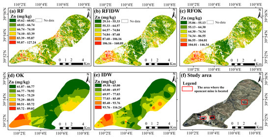
Figure 9.
Spatial distribution maps of Zn contents in the research area.
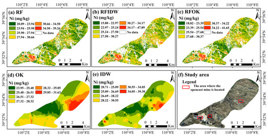
Figure 10.
Spatial distribution maps of Ni contents in the study area.
In this study, R2, RMSE, and MAE were adopted to evaluate heavy metal concentration map accuracy, and 30% of soil samples were defined as the validation sets (Table 2).
Table 2.
Heavy metal concentrations map accuracy evaluation.
Clearly, the RFOK method demonstrated the best accuracy with the highest validation R2 (0.6029 for Zn, 0.3038 for Ni) and the lowest validation RMSE (12.4515 mg/kg for Zn, 3.9765 mg/kg for Ni) and MAE (9.4730 mg/kg for Zn, 3.3112 mg/kg for Ni) for both Zn and Ni (Table 2 and Figure 8).
Hence, the RFOK was selected as the final method to map the heavy metal concentrations in this study (Figure 9c and Figure 10c).
A published study has found that several variables, including topography, human activities, and the distribution of pollution sources, may impose effects on the distribution of heavy metals [74].
Although this study only selected spectral data as the independent variables, and the impact of environmental conditions on the distribution of soil heavy metals was ignored, the two-stage scheme compensated for this flaw, to some extent.
The RF model can determine the relationship between heavy metal concentrations and spectral reflectance [75]. However, the influence of environmental factors and topography factors on the heavy metal concentrations was completely ignored by the RF model.
The geo-statistical models, such as OK and IDW, based on the first law of geography, can reflect the relationship between heavy metal contents and environmental factors.
Thus, both RF and geostatistical models were merged in this study, and the results confirmed that this two-stage scheme can be adopted to predict heavy metal concentrations.
3.5. Distribution Feature of Toxic Metals
To compare the reliability of heavy metal concentrations distribution maps, five maps generated by RF, RFIDW, RFOK, OK, and IDW, are shown simultaneously (Figure 9 and Figure 10). Figure 9f and Figure 10f are true-color GF-5 images of the study area.
As demonstrated in Figure 8 and Figure 9, the heavy metal concentrations distribution map based on five methods for both Zn and Ni are comparable, and the spatial distribution features are largely consistent.
Clearly, the concentrations for both Zn and Ni exceeded the local heavy metal concentrations background value, but were lower than the limits contained in the Chinese criteria in most locations of the study area (Figure 9 and Figure 10 and Table 1). Two hotspots for Zn and Ni were detected, respectively, in the southwest and the middle east portions of the study area because the largest opencast coal mine, as well as a number of other coal mines, are mainly distributed in the southwest and the middle east portions of the study area. These results confirmed that the development of the opencast coal mine generated obvious influences on the distribution of heavy metals in the area.
It is clear that the spatial distributions of Zn and Ni were approximately the same, while the detailed descriptions of each map vary to some extent (Figure 9 and Figure 10).
Specifically, the geographical distribution maps generated by the geostatistical models, with discontinuities in the transition zones of heavy metals, are similar (Figure 9d,e and Figure 10d,e). The spatial variability can scarcely be represented by the geographical distribution maps.
By contrast, the RF method can construct a quantitative relationship between heavy metal concentrations and spectral data, and the spatial distribution of heavy metal concentrations can be explicitly described using GF-5 images based on RF at the raster scale.
However, the influence of environmental factors such as geographical location on the predicted results were not considered by the RF. Hence, the two-staged schemes proposed by this study, integrating geostatistical methods with RF, can compensate for the disadvantage of the RF model and improve the overall precision. The distribution maps of heavy metal concentrations generated by RFOK demonstrated more objectivity than other methods, according to performance evaluation (Table 2, Figure 9c and Figure 10c).
4. Conclusions
By combining the heavy metal concentrations at the sampling sites with the GF-5 hyperspectral image, this study proposes a two-stage scheme to directly map the spatial distribution of heavy metal contents without surveying the spectral data. Heavy metal concentration maps were indirectly inferred based on the close relationship between heavy metals and SOC and clay. The findings of this study indicated that it is possible to acquire the spatial distribution of heavy metals using hyperspectral images directly based on the close relationship between heavy metals and related soil materials, such as SOC and clay, over a relatively larger area.
The average concentration of Zn and Ni are 68.07 mg/kg and 26.61 mg/kg in the study area, respectively, which are higher than the concentrations in the regional background values.
Additionally, this study integrates geostatistical methods with RF to develop a two-stage scheme for estimating heavy metal concentrations, and the prediction accuracy improved significantly because both the spectral characteristic of heavy metals and the influence of environmental factors were taken into consideration via the two-stage scheme.
The features of the distribution of the heavy metals estimated by five prediction methods were detected to be close, while exhibiting a significant difference in details. The heterogeneity of heavy metals distribution and the concentrations in the transition regions can be well described by the RFOK model. On the contrary, the capacity and accuracy of the other four methods regarding capturing the detailed spatial variability of toxic metals are relatively weak.
The mechanism of the distribution of heavy metals is quite complicated. Although the two-staged schemes can be carried out to estimate toxic metal concentrations, the inner mechanism is still uncertain. Therefore, we plan to conduct a new quantitative study to explore the sources of heavy metals and the influence of environmental factors regarding heavy metals in the coal mining areas.
Supplementary Materials
The following supporting information can be downloaded at: https://www.mdpi.com/article/10.3390/rs14225804/s1, Figure S1: Testing diagram of SG Window Length; Table S1: Accuracy evaluation of different spectra pretreatment methods.
Author Contributions
Conceptualization, B.G. and X.G.; methodology, B.G. and B.Z.; software, L.S.; validation, B.G. and X.G.; formal analysis, B.G. and L.S.; investigation, X.G. and B.Z.; resources, X.G. and B.Z.; data curation, B.G. and L.S.; writing—original draft preparation, B.G. and X.G.; writing—review and editing, X.G. and H.B.; visualization, B.G. and P.L.; supervision, X.G. and P.L.; project administration, B.G. and H.B.; funding acquisition, X.G. and H.B. All authors have read and agreed to the published version of the manuscript.
Funding
This research was funded by the Foundation of Shaanxi Key Laboratory of Land Consolidation of Chang’an University (300102352505), the Open Foundation of the State Key Laboratory of Urban and Regional Ecology of China (SKLURE 2021-2-6), and the Natural Science Foundation of Shaanxi Province (2021JM-388).
Data Availability Statement
The data presented in this study are available on request from the corresponding author. The data are not publicly available due to privacy restrictions. The code used in this study is available on request from the corresponding author.
Conflicts of Interest
The authors declare no conflict of interest. The funders had no role in the design of the study; in the collection, analysis, or interpretation of data; in the writing of the manuscript; or in the decision to publish the results.
References
- Yin, G.; Chen, X.; Zhu, H.; Chen, Z.; Su, C.; He, Z.; Qiu, J.; Wang, T. A novel interpolation method to predict soil heavy metals based on a genetic algorithm and neural network model. Sci. Total Environ. 2022, 825, 153948. [Google Scholar] [CrossRef] [PubMed]
- Fu, P.; Yang, K.; Meng, F.; Zhang, W.; Cui, Y.; Feng, F.; Yao, G. A new three-band spectral and metal element index for estimating soil arsenic content around the mining area. Process Saf. Environ. 2022, 157, 27–36. [Google Scholar] [CrossRef]
- Ou, D.; Tan, K.; Wang, X.; Wu, Z.; Li, J.; Ding, J. Modified soil scattering coefficients for organic matter inversion based on Kubelka-Munk theory. Geoderma 2022, 418, 115845. [Google Scholar] [CrossRef]
- Zhou, W.; Yang, H.; Xie, L.; Li, H.; Huang, L.; Zhao, Y.; Yue, T. Hyperspectral inversion of soil heavy metals in Three-River Source Region based on random forest model. Catena 2021, 202, 105222. [Google Scholar] [CrossRef]
- Ou, D.; Tan, K.; Lai, J.; Jia, X.; Wang, X.; Chen, Y.; Li, J. Semi-supervised DNN regression on airborne hyperspectral imagery for improved spatial soil properties prediction. Geoderma 2021, 385, 114875. [Google Scholar] [CrossRef]
- Zou, B.; Jiang, X.; Feng, H.; Tu, Y.; Tao, C. Multisource spectral-integrated estimation of cadmium concentrations in soil using a direct standardization and Spiking algorithm. Sci. Total Environ. 2020, 701, 134890. [Google Scholar] [CrossRef]
- Wang, N.; Guan, Q.; Sun, Y.; Wang, B.; Ma, Y.; Shao, W.; Li, H. Predicting the spatial pollution of soil heavy metals by using the distance determination coefficient method. Sci. Total Environ. 2021, 799, 149452. [Google Scholar] [CrossRef]
- Zhang, B.; Guo, B.; Zou, B.; Wei, W.; Lei, Y.; Li, T. Retrieving soil heavy metals concentrations based on GaoFen-5 hyperspectral satellite image at an opencast coal mine, Inner Mongolia, China. Environ. Pollut. 2022, 300, 118981. [Google Scholar] [CrossRef]
- Guo, B.; Zhang, B.; Su, Y.; Zhang, D.; Wang, Y.; Bian, Y.; Suo, L.; Guo, X.; Bai, H. Retrieving zinc concentrations in topsoil with reflectance spectroscopy at Opencast Coal Mine sites. Sci. Rep. 2021, 11, 19909. [Google Scholar] [CrossRef]
- Yin, F.; Wu, M.; Liu, L.; Zhu, Y.; Feng, J.; Yin, D.; Yin, C.; Yin, C. Predicting the abundance of copper in soil using reflectance spectroscopy and GF5 hyperspectral imagery. Int. J. Appl. Earth Obs. 2021, 102, 102420. [Google Scholar] [CrossRef]
- Xu, D.; Chen, S.; Xu, H.; Wang, N.; Zhou, Y.; Shi, Z. Data fusion for the measurement of potentially toxic elements in soil using portable spectrometers. Environ. Pollut. 2020, 263, 114649. [Google Scholar] [CrossRef] [PubMed]
- Wang, Y.; Zhang, X.; Sun, W.; Wang, J.; Ding, S.; Liu, S. Effects of hyperspectral data with different spectral resolutions on the estimation of soil heavy metal content: From ground-based and airborne data to satellite-simulated data. Sci. Total Environ. 2022, 838, 156129. [Google Scholar] [CrossRef] [PubMed]
- Hong, Y.; Chen, Y.; Shen, R.; Chen, S.; Xu, G.; Cheng, H.; Guo, L.; Wei, Z.; Yang, J.; Liu, Y.; et al. Diagnosis of cadmium contamination in urban and suburban soils using visible-to-near-infrared spectroscopy. Environ. Pollut. 2021, 291, 118128. [Google Scholar] [CrossRef]
- Guo, B.; Su, Y.; Pei, L.; Wang, X.; Zhang, B.; Zhang, D.; Wang, X. Ecological risk evaluation and source apportionment of heavy metals in park playgrounds: A case study in Xi’an, Shaanxi Province, a northwest city of China. Environ. Sci. Pollut. Res. 2020, 27, 24400–24412. [Google Scholar] [CrossRef]
- Guo, B.; Su, Y.; Pei, L.; Wang, X.; Wei, X.; Zhang, B.; Zhang, D.; Wang, X. Contamination, Distribution and Health Risk Assessment of Risk Elements in Topsoil forAmusement Parks in Xi’an, China. Pol. J. Environ. Stud. 2021, 30, 601–617. [Google Scholar] [CrossRef]
- Chen, L.; Lai, J.; Tan, K.; Wang, X.; Chen, Y.; Ding, J. Development of a soil heavy metal estimation method based on a spectral index: Combining fractional-order derivative pretreatment and the absorption mechanism. Sci. Total Environ. 2022, 813, 151882. [Google Scholar] [CrossRef]
- Han, C.; Lu, J.; Chen, S.; Xu, X.; Wang, Z.; Pei, Z.; Zhang, Y.; Li, F. Estimation of Heavy Metal(Loid) Contents in Agricultural Soil of the Suzi River Basin Using Optimal Spectral Indices. Sustainability 2021, 13, 12088. [Google Scholar] [CrossRef]
- Zhang, S.; Fei, T.; Chen, Y.; Hong, Y. Estimating cadmium-lead concentrations in rice blades through fractional order derivatives of foliar spectra. Biosyst. Eng. 2022, 219, 177–188. [Google Scholar] [CrossRef]
- Liu, W.; Yu, Q.; Niu, T.; Yang, L.; Liu, H. Inversion of Soil Heavy Metal Content Based on Spectral Characteristics of Peach Trees. Forests 2021, 12, 1208. [Google Scholar] [CrossRef]
- Meng, X.; Bao, Y.; Ye, Q.; Liu, H.; Zhang, X.; Tang, H.; Zhang, X. Soil Organic Matter Prediction Model with Satellite Hyperspectral Image Based on Optimized Denoising Method. Remote Sens. 2021, 13, 2273. [Google Scholar] [CrossRef]
- Tu, Y.; Zou, B.; Feng, H.; Zhou, M.; Yang, Z.; Xiong, Y. A Near Standard Soil Samples Spectra Enhanced Modeling Strategy for Cd Concentration Prediction. Remote Sens. 2021, 13, 2657. [Google Scholar] [CrossRef]
- Wang, Y.; Yu, T.; Yang, Z.; Bo, H.; Lin, Y.; Yang, Q.; Liu, X.; Zhang, Q.; Zhuo, X.; Wu, T. Zinc concentration prediction in rice grain using back-propagation neural network based on soil properties and safe utilization of paddy soil: A large-scale field study in Guangxi, China. Sci. Total Environ. 2021, 798, 149270. [Google Scholar] [CrossRef] [PubMed]
- Lin, D.; Li, G.; Zhu, Y.; Liu, H.; Li, L.; Fahad, S.; Zhang, X.; Wei, C.; Jiao, Q. Predicting copper content in chicory leaves using hyperspectral data with continuous wavelet transforms and partial least squares. Comput. Electron. Agric. 2021, 187, 106293. [Google Scholar] [CrossRef]
- Khosravi, V.; Ardejani, F.D.; Gholizadeh, A.; Saberioon, M. Satellite Imagery for Monitoring and Mapping Soil Chromium Pollution in a Mine Waste Dump. Remote Sens. 2021, 13, 1277. [Google Scholar] [CrossRef]
- Khosravi, V.; Doulati Ardejani, F.; Yousefi, S.; Aryafar, A. Monitoring soil lead and zinc contents via combination of spectroscopy with extreme learning machine and other data mining methods. Geoderma 2018, 318, 29–41. [Google Scholar] [CrossRef]
- Tan, K.; Ma, W.; Chen, L.; Wang, H.; Du, Q.; Du, P.; Yan, B.; Liu, R.; Li, H. Estimating the distribution trend of soil heavy metals in mining area from HyMap airborne hyperspectral imagery based on ensemble learning. J. Hazard. Mater. 2021, 401, 123288. [Google Scholar] [CrossRef]
- Jia, X.; Cao, Y.; O’Connor, D.; Zhu, J.; Tsang, D.; Zou, B.; Hou, D. Mapping soil pollution by using drone image recognition and machine learning at an arsenic-contaminated agricultural field. Environ. Pollut. 2021, 270, 116281. [Google Scholar] [CrossRef]
- Ye, B.; Tian, S.; Cheng, Q.; Ge, Y. Application of Lithological Mapping Based on Advanced Hyperspectral Imager (AHSI) Imagery Onboard Gaofen-5 (GF-5) Satellite. Remote Sens. 2020, 12, 3990. [Google Scholar] [CrossRef]
- Jiang, G.; Zhou, S.; Cui, S.; Chen, T.; Wang, J.; Chen, X.; Liao, S.; Zhou, K. Exploring the Potential of HySpex Hyperspectral Imagery for Extraction of Copper Content. Sensors 2020, 20, 6325. [Google Scholar] [CrossRef]
- Guo, B.; Zhang, D.; Zhang, D.; Su, Y.; Wang, X.; Bian, Y. Detecting Spatiotemporal Dynamic of Regional Electric Consumption Using NPP-VIIRS Nighttime Stable Light Data—A Case Study of Xi’an, China. IEEE Access 2020, 8, 171694–171702. [Google Scholar] [CrossRef]
- Jia, X.; O’Connor, D.; Shi, Z.; Hou, D. VIRS based detection in combination with machine learning for mapping soil pollution. Environ. Pollut. 2020, 268, 115845. [Google Scholar] [CrossRef] [PubMed]
- Gholizadeh, A.; Saberioon, M.; Ben-Dor, E.; Viscarra Rossel, R.A.; Borůvka, L. Modelling potentially toxic elements in forest soils with vis–NIR spectra and learning algorithms. Environ. Pollut. 2020, 267, 115574. [Google Scholar] [CrossRef]
- Shi, T.; Yang, C.; Liu, H.; Wu, C.; Wang, Z.; Li, H.; Zhang, H.; Guo, L.; Wu, G.; Su, F. Mapping lead concentrations in urban topsoil using proximal and remote sensing data and hybrid statistical approaches. Environ. Pollut. 2021, 272, 116041. [Google Scholar] [CrossRef] [PubMed]
- He, M.; Yan, P.; Yu, H.; Yang, S.; Xu, J.; Liu, X. Spatiotemporal modeling of soil heavy metals and early warnings from scenarios-based prediction. Chemosphere 2020, 255, 126908. [Google Scholar] [CrossRef] [PubMed]
- Zhang, H.; Yin, S.; Chen, Y.; Shao, S.; Wu, J.; Fan, M.; Chen, F.; Gao, C. Machine learning-based source identification and spatial prediction of heavy metals in soil in a rapid urbanization area, eastern China. J. Clean. Prod. 2020, 273, 122858. [Google Scholar] [CrossRef]
- Wu, Z.; Lei, S.; Lu, Q.; Bian, Z. Impacts of Large-Scale Open-Pit Coal Base on the Landscape Ecological Health of Semi-Arid Grasslands. Remote Sens. 2019, 11, 1820. [Google Scholar] [CrossRef]
- Ding, S.; Zhang, X.; Sun, W.; Shang, K.; Wang, Y. Estimation of soil lead content based on GF-5 hyperspectral images, considering the influence of soil environmental factors. J. Soils Sediments 2022, 22, 1431–1445. [Google Scholar] [CrossRef]
- Sun, W.; Liu, S.; Zhang, X.; Zhu, H. Performance of hyperspectral data in predicting and mapping zinc concentration in soil. Sci. Total Environ. 2022, 824, 153766. [Google Scholar] [CrossRef]
- Guo, B.; Zhang, D.; Pei, L.; Su, Y.; Wang, X.; Bian, Y.; Zhang, D.; Yao, W.; Zhou, Z.; Guo, L. Estimating PM2.5 concentrations via random forest method using satellite, auxiliary, and ground-level station dataset at multiple temporal scales across China in 2017. Sci. Total Environ. 2021, 778, 146288. [Google Scholar] [CrossRef]
- Salminen, R.; Tarvainen, T.; Demetriades, A.; Duris, M.; Fordyce, F.M.; Gregorauskiene, V.; Kahelin, H.; Kivisilla, J.; Klaver, G.; Klein, H.; et al. FOREGS Geochemical Mapping Field Manual; Opas–Geologian Tutkimuskeskus; ResearchGate: Berlin, Germany, 1998. [Google Scholar]
- Tan, K.; Wang, X.; Niu, C.; Wang, F.; Du, P.; Sun, D.; Yuan, J.; Zhang, J. Vicarious Calibration for the AHSI Instrument of Gaofen-5 with Reference to the CRCS Dunhuang Test Site. IEEE Trans. Geosci. Remote Sens. 2021, 59, 3409–3419. [Google Scholar] [CrossRef]
- Kordestani, H.; Zhang, C. Direct Use of the Savitzky–Golay Filter to Develop an Output-Only Trend Line-Based Damage Detection Method. Sensors 2020, 20, 1983. [Google Scholar] [CrossRef] [PubMed]
- Zhang, S.; Shen, Q.; Nie, C.; Huang, Y.; Wang, J.; Hu, Q.; Ding, X.; Zhou, Y.; Chen, Y. Hyperspectral inversion of heavy metal content in reclaimed soil from a mining wasteland based on different spectral transformation and modeling methods. Spectrochim. Acta Part A Mol. Biomol. Spectrosc. 2019, 211, 393–400. [Google Scholar] [CrossRef] [PubMed]
- Wu, Q.; Xu, H. Design and development of an on-line fluorescence spectroscopy system for detection of aflatoxin in pistachio nuts. Postharvest Biol. Technol. 2020, 159, 111016. [Google Scholar] [CrossRef]
- Wei, L.; Pu, H.; Wang, Z.; Yuan, Z.; Yan, X.; Cao, L. Estimation of Soil Arsenic Content with Hyperspectral Remote Sensing. Sensors 2020, 20, 4056. [Google Scholar] [CrossRef] [PubMed]
- Xu, X.; Ren, M.; Cao, J.; Wu, Q.; Liu, P.; Lv, J. Spectroscopic diagnosis of zinc contaminated soils based on competitive adaptive reweighted sampling algorithm and an improved support vector machine. Spectrosc. Lett. 2020, 53, 86–99. [Google Scholar] [CrossRef]
- Garg, S.; Kaur, K.; Batra, S.; Kaddoum, G.; Kumar, N.; Boukerche, A. A multi-stage anomaly detection scheme for augmenting the security in IoT-enabled applications. Futur. Gener. Comput. Syst. 2020, 104, 105–118. [Google Scholar] [CrossRef]
- Hasan, M.J.; Kim, J.; Kim, C.H.; Kim, J. Health State Classification of a Spherical Tank Using a Hybrid Bag of Features and K-Nearest Neighbor. Appl. Sci. 2020, 10, 2525. [Google Scholar] [CrossRef]
- Tan, K.; Wang, H.; Chen, L.; Du, Q.; Du, P.; Pan, C. Estimation of the spatial distribution of heavy metal in agricultural soils using airborne hyperspectral imaging and random forest. J. Hazard. Mater. 2020, 382, 120987. [Google Scholar] [CrossRef]
- Guo, B.; Wu, H.; Pei, L.; Zhu, X.; Zhang, D.; Wang, Y.; Luo, P. Study on the spatiotemporal dynamic of ground-level ozone concentrations on multiple scales across China during the blue sky protection campaign. Environ. Int. 2022, 170, 107606. [Google Scholar] [CrossRef]
- Meng, X.; Bao, Y.; Liu, J.; Liu, H.; Zhang, X.; Zhang, Y.; Wang, P.; Tang, H.; Kong, F. Regional soil organic carbon prediction model based on a discrete wavelet analysis of hyperspectral satellite data. Int. J. Appl. Earth Obs. 2020, 89, 102111. [Google Scholar] [CrossRef]
- Guo, B.; Bian, Y.; Zhang, D.; Su, Y.; Wang, X.; Zhang, B.; Wang, Y.; Chen, Q.; Wu, Y.; Luo, P. Estimating Socio-Economic Parameters via Machine Learning Methods Using Luojia1-01 Nighttime Light Remotely Sensed Images at Multiple Scales of China in 2018. IEEE Access 2021, 9, 34352–34365. [Google Scholar] [CrossRef]
- Hong, Y.; Guo, L.; Chen, S.; Linderman, M.; Mouazen, A.M.; Yu, L.; Chen, Y.; Liu, Y.; Liu, Y.; Cheng, H.; et al. Exploring the potential of airborne hyperspectral image for estimating topsoil organic carbon: Effects of fractional-order derivative and optimal band combination algorithm. Geoderma 2020, 365, 114228. [Google Scholar] [CrossRef]
- Wang, L.; Zhou, Y.; Liu, J.; Liu, Y.; Zuo, Q.; Li, Q. Exploring the potential of multispectral satellite images for estimating the contents of cadmium and lead in cropland: The effect of the dimidiate pixel model and random forest. J. Clean. Prod. 2022, 367, 132922. [Google Scholar] [CrossRef]
- Guo, B.; Wang, Y.; Pei, L.; Yu, Y.; Liu, F.; Zhang, D.; Wang, X.; Su, Y.; Zhang, D.; Zhang, B.; et al. Determining the effects of socioeconomic and environmental determinants on chronic obstructive pulmonary disease (COPD) mortality using geographically and temporally weighted regression model across Xi’an during 2014–2016. Sci. Total Environ. 2021, 756, 143869. [Google Scholar] [CrossRef] [PubMed]
- Guo, B.; Wang, X.; Pei, L.; Su, Y.; Zhang, D.; Wang, Y. Identifying the spatiotemporal dynamic of PM2.5 concentrations at multiple scales using geographically and temporally weighted regression model across China during 2015–2018. Sci. Total Environ. 2021, 751, 141765. [Google Scholar] [CrossRef]
- Guo, B.; Wang, X.; Zhang, D.; Pei, L.; Zhang, D.; Wang, X. A Land Use Regression Application into SimulatingSpatial Distribution Characteristics of ParticulateMatter (PM2.5) Concentration in Cityof Xi’an, China. Pol. J. Environ. Stud. 2020, 29, 4065–4076. [Google Scholar] [CrossRef]
- Golden, N.; Zhang, C.; Potito, A.; Gibson, P.J.; Bargary, N.; Morrison, L. Use of ordinary cokriging with magnetic susceptibility for mapping lead concentrations in soils of an urban contaminated site. J. Soil. Sediment. 2020, 20, 1357–1370. [Google Scholar] [CrossRef]
- Külahcı, F.; Şen, Z. Cumulative Ordinary Kriging interpolation model to forecast radioactive fallout, and its application to Chernobyl and Fukushima assessment: A new method and mini review. Environ. Sci. Pollut. Res. 2022, 29, 64298–64311. [Google Scholar] [CrossRef]
- Wang, Q.; Xiao, H.; Wu, W.; Su, F.; Zuo, X.; Yao, G.; Zheng, G. Reconstructing High-Precision Coral Reef Geomorphology from Active Remote Sensing Datasets: A Robust Spatial Variability Modified Ordinary Kriging Method. Remote Sens. 2022, 14, 253. [Google Scholar] [CrossRef]
- Qu, R.; Hou, H.; Xiao, K.; Liu, B.; Liang, S.; Hu, J.; Bian, S.; Yang, J. Prediction on the combined toxicities of stimulation-only and inhibition-only contaminants using improved inverse distance weighted interpolation. Chemosphere 2022, 287, 132045. [Google Scholar] [CrossRef] [PubMed]
- Khouni, I.; Louhichi, G.; Ghrabi, A. Use of GIS based Inverse Distance Weighted interpolation to assess surface water quality: Case of Wadi El Bey, Tunisia. Environ. Technol. Innov. 2021, 24, 101892. [Google Scholar] [CrossRef]
- Liu, G.; Zhou, X.; Li, Q.; Shi, Y.; Guo, G.; Zhao, L.; Wang, J.; Su, Y.; Zhang, C. Spatial distribution prediction of soil As in a large-scale arsenic slag contaminated site based on an integrated model and multi-source environmental data. Environ. Pollut. 2020, 267, 115631. [Google Scholar] [CrossRef]
- Lin, N.; Jiang, R.; Li, G.; Yang, Q.; Li, D.; Yang, X. Estimating the heavy metal contents in farmland soil from hyperspectral images based on Stacked AdaBoost ensemble learning. Ecol. Indic. 2022, 143, 109330. [Google Scholar] [CrossRef]
- State Environmental Protection Administration; China National Environmental Monitoring Centre. Background Values of Soil Elements in China; China Environmental Science Press: Beijing, China, 1990. [Google Scholar]
- Sun, W.; Zhang, X.; Sun, X.; Sun, Y.; Cen, Y. Predicting nickel concentration in soil using reflectance spectroscopy associated with organic matter and clay minerals. Geoderma 2018, 327, 25–35. [Google Scholar] [CrossRef]
- Lu, Q.; Wang, S.; Bai, X.; Liu, F.; Wang, M.; Wang, J.; Tian, S. Rapid inversion of heavy metal concentration in karst grain producing areas based on hyperspectral bands associated with soil components. Microchem. J. 2019, 148, 404–411. [Google Scholar] [CrossRef]
- Rivard, B.; Feng, J.; Gallie, A.; Sanchez-Azofeifa, A. Continuous wavelets for the improved use of spectral libraries and hyperspectral data. Remote Sens. Environ. 2008, 112, 2850–2862. [Google Scholar] [CrossRef]
- Song, Y.-Q.; Zhu, A.-X.; Cui, X.-S.; Liu, Y.-L.; Hu, Y.-M.; Li, B. Spatial variability of selected metals using auxiliary variables in agricultural soils. Catena 2019, 174, 499–513. [Google Scholar] [CrossRef]
- Hong, Y.; Chen, S.; Chen, Y.; Linderman, M.; Mouazen, A.M.; Liu, Y.; Guo, L.; Yu, L.; Liu, Y.; Cheng, H.; et al. Comparing laboratory and airborne hyperspectral data for the estimation and mapping of topsoil organic carbon: Feature selection coupled with random forest. Soil Tillage Res. 2020, 199, 104589. [Google Scholar] [CrossRef]
- Liu, Z.; Lu, Y.; Peng, Y.; Zhao, L.; Wang, G.; Hu, Y. Estimation of Soil Heavy Metal Content Using Hyperspectral Data. Remote Sens. 2019, 11, 1464. [Google Scholar] [CrossRef]
- Hong, Y.; Chen, S.; Liu, Y.; Zhang, Y.; Yu, L.; Chen, Y.; Liu, Y.; Cheng, H.; Liu, Y. Combination of fractional order derivative and memory-based learning algorithm to improve the estimation accuracy of soil organic matter by visible and near-infrared spectroscopy. Catena 2019, 174, 104–116. [Google Scholar] [CrossRef]
- Taghizadeh-Mehrjardi, R.; Fathizad, H.; Ali Hakimzadeh Ardakani, M.; Sodaiezadeh, H.; Kerry, R.; Heung, B.; Scholten, T. Spatio-Temporal Analysis of Heavy Metals in Arid Soils at the Catchment Scale Using Digital Soil Assessment and a Random Forest Model. Remote Sens. 2021, 13, 1698. [Google Scholar] [CrossRef]
- Sun, W.; Zhang, X. Estimating soil zinc concentrations using reflectance spectroscopy. Int. J. Appl. Earth Obs. 2017, 58, 126–133. [Google Scholar] [CrossRef]
- Cheng, Y.; Zhou, Y. Research progress and trend of hyperspectral remote sensing quantitative monitoring of soil heavy metals. Chin. J. Nonferr. Met. 2021, 11, 3450–3467. [Google Scholar]
Publisher’s Note: MDPI stays neutral with regard to jurisdictional claims in published maps and institutional affiliations. |
© 2022 by the authors. Licensee MDPI, Basel, Switzerland. This article is an open access article distributed under the terms and conditions of the Creative Commons Attribution (CC BY) license (https://creativecommons.org/licenses/by/4.0/).