
Supervised Segmentation of NO2 Plumes from Individual Ships Using TROPOMI Satellite Data

 ,
,
Abstract
1. Introduction
2. Related Work
3. Materials and Methods
3.1. Data Sources
3.1.1. TROPOMI Data
3.1.2. Wind Data
3.1.3. Ship-Related Data
3.2. Method
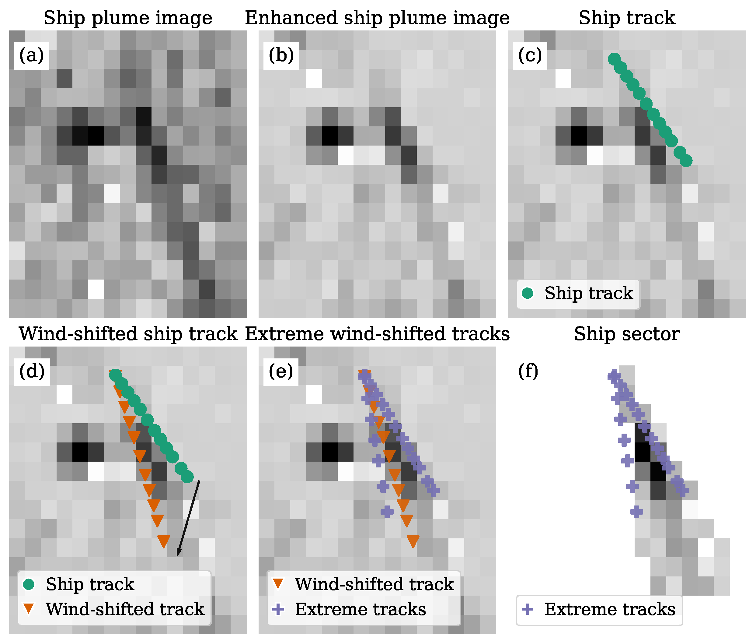
3.2.1. Ship Tracks
3.2.2. Ship Plume Image
3.2.3. Pre-Processing of a Ship Plume Image
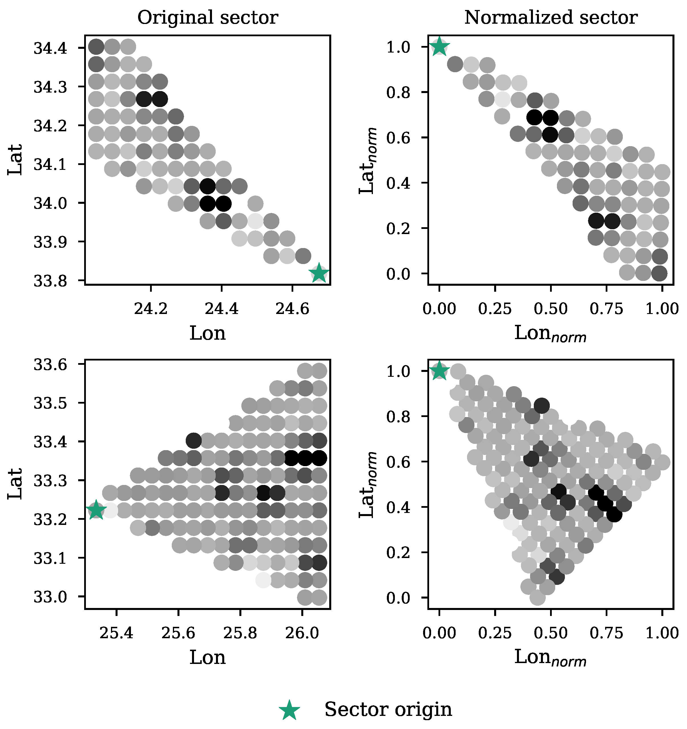
3.2.4. Ship Sector
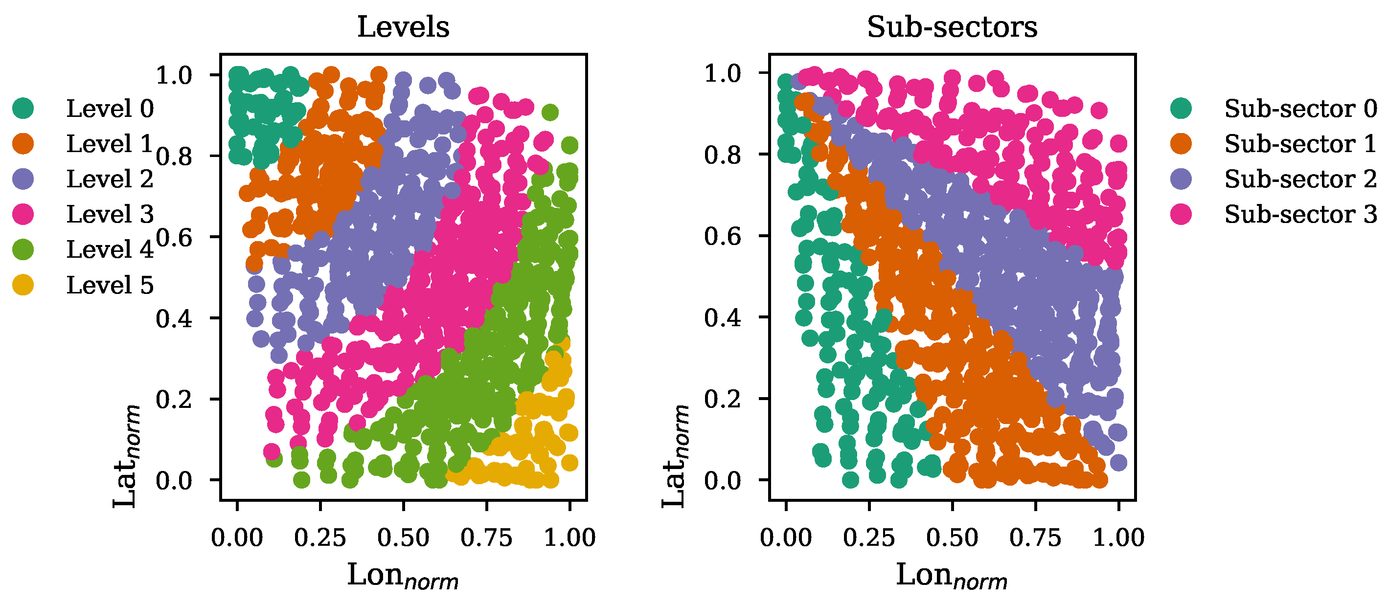
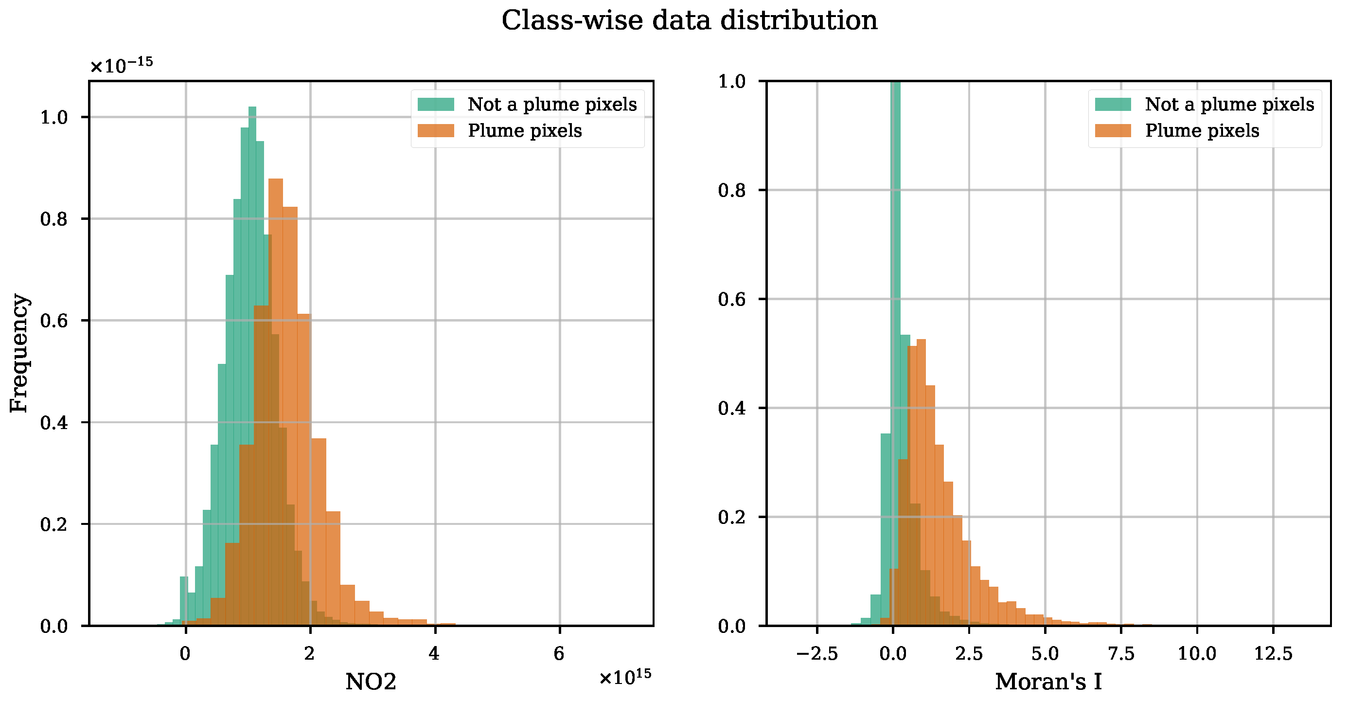
3.2.5. Feature Set Construction
3.3. Experiment Design
3.3.1. Dataset Composition
3.3.2. Multivariate Models
3.3.3. Benchmarks
3.3.4. Segmentation Validation Metrics
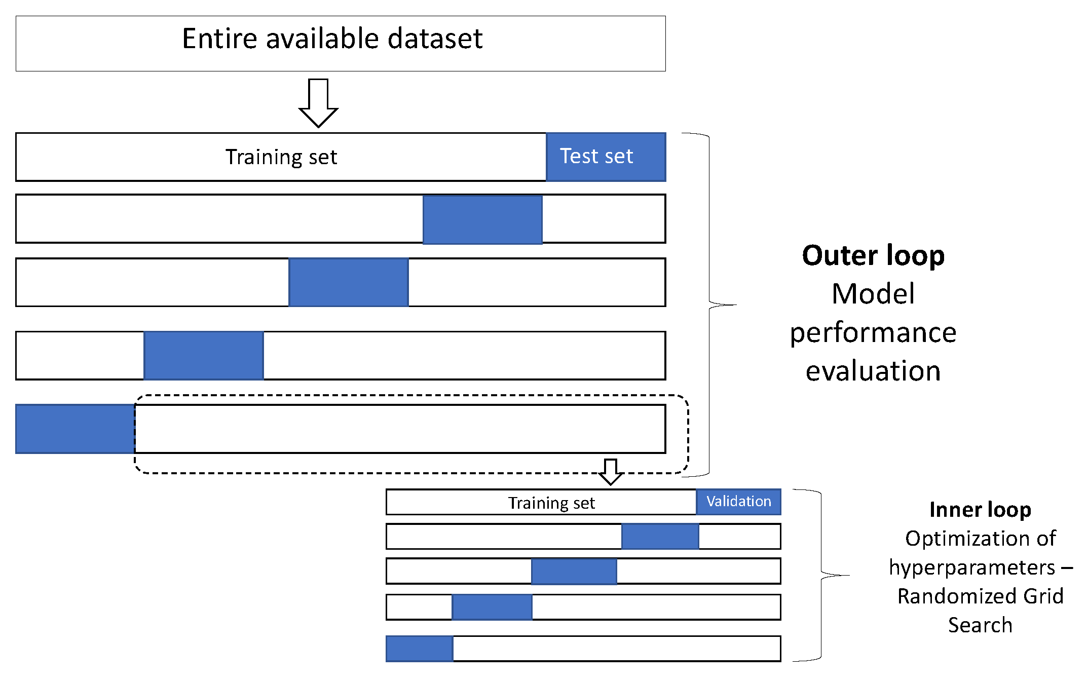
3.3.5. Cross-Validation and Parameters’ Optimization
3.3.6. Validation Metrics
4. Results
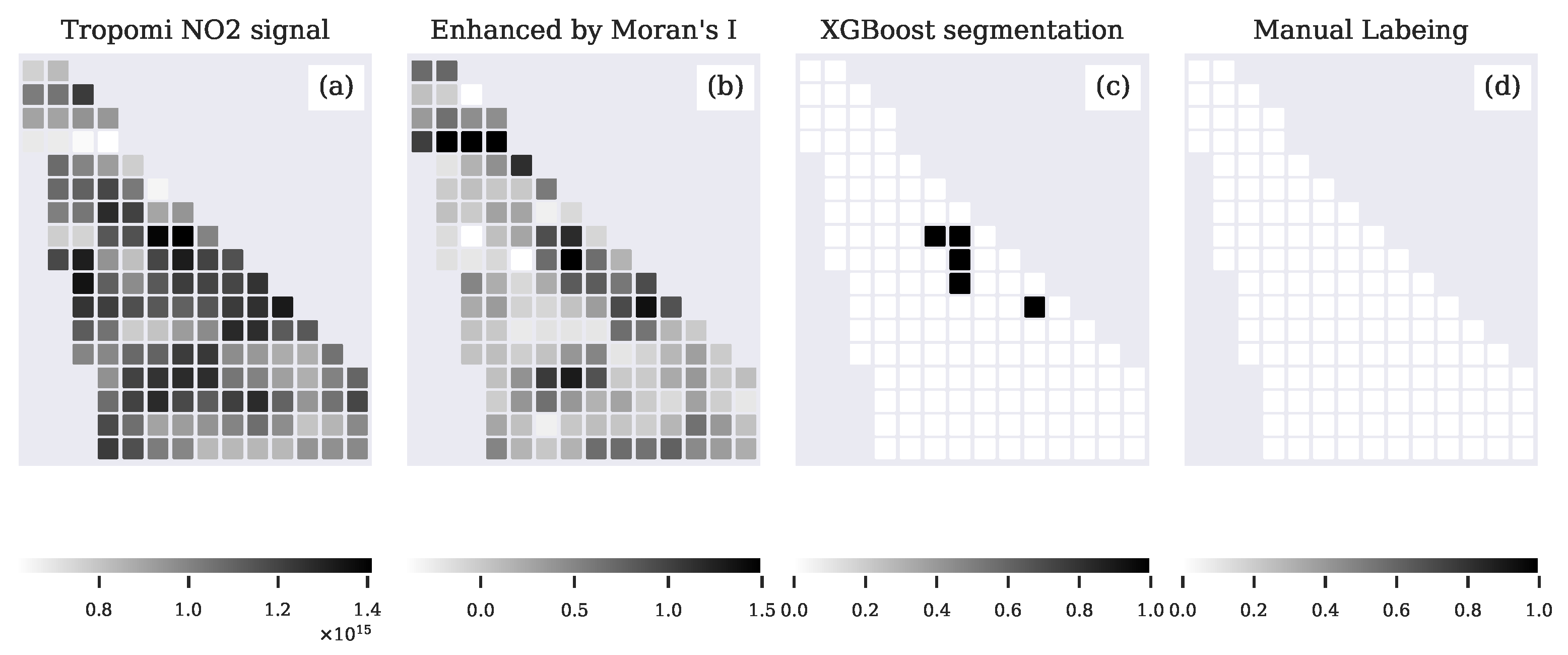
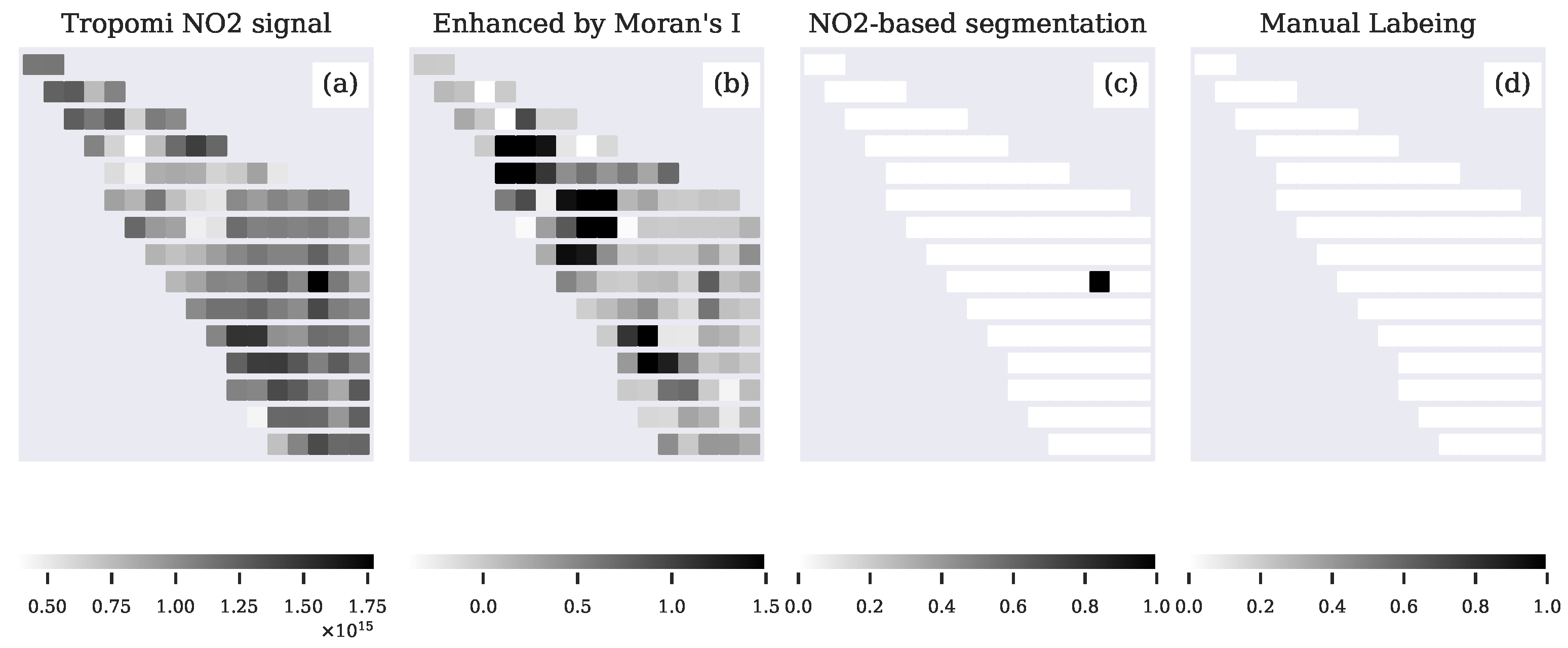
4.1. Plume Segmentation
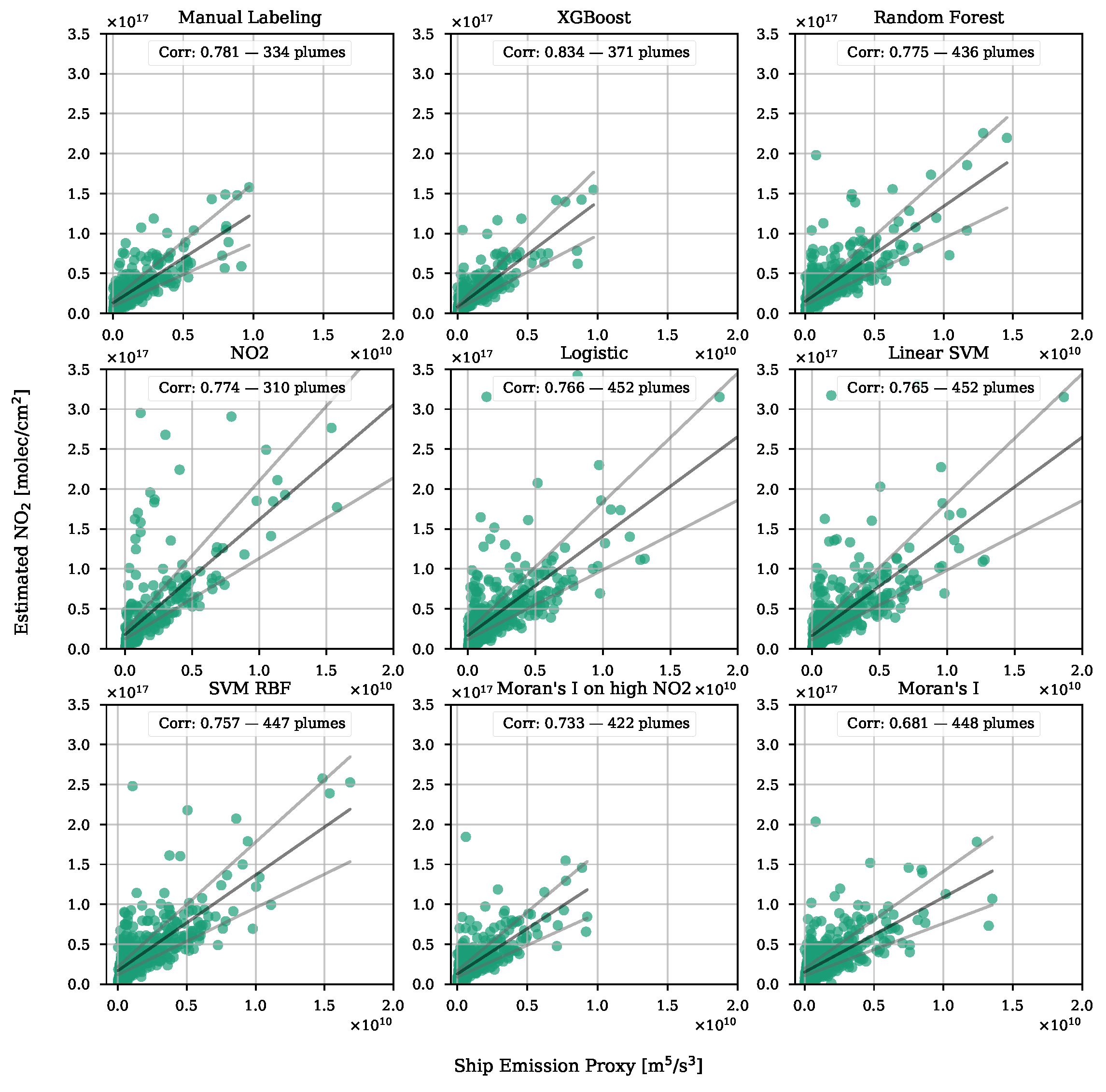
4.2. Validation with Emission Proxy
5. Conclusions
6. Discussion
Author Contributions
Funding
Data Availability Statement
Acknowledgments
Conflicts of Interest
Abbreviations
| S5P | Copernicus Sentinel 5 Precursor satellite |
| Nitrogen dioxide | |
| ECMWF | European Center for Medium-range Weather Forecast |
| AIS | Automatic Identification System |
| ILT | Human Environment and Transport Inspectorate of the Netherlands |
| ROI | Region Of Interest |
| SVM | Support Vector Machine |
| RBF SVM | Support Vector Machine with Radial Basis Kernel |
| XGBoost | Extreme Gradient Boosting |
| AP | Average Precision |
Appendix A. Hyperparameters Settings
- Linear SVM( = 0)
- -
- C: (, , , , )
- Logistic( = ‘saga’, = 0.5, = 0)
- -
- : (‘l1’, ‘l2’, ‘elasticnet’, ‘none’)
- -
- C: (0.0001, 0.001, 0.1, 1)
- -
- : (100, 120, 150)
- RBF SVM( = ‘rbf’, = ‘scale’, = 0)
- -
- C: (, , , , , , )
- Random Forest( = 500, = True,= 0)
- -
- : [2; 36]
- -
- : (‘sqrt’, 0.4, 0.5)
- -
- : (‘gini’, ‘entropy’)
- XGBoost( = ‘binary:logistic’, = ‘aucpr’,= 500, = ‘gbtree’, = 0)
- -
- : [0.05; 0.5]
- -
- : (2, 3, 5, 6)
- -
- : (2, 4, 6, 8, 10, 12)
- -
- : [0.6; 1.0]
- -
- : [0.6; 1.0]
- -
- : [0.6; 1.0]
- -
- : (0.001, 0.01, 0.1, 0.2, 0.3, 0.4)
- -
- : (0, , , , , , )
Appendix B. Hyperparameters Selected by the Optimization Process
- Linear SVM: In every iteration of the cross-validation procedure, the optimal value of parameter C was: C = 0.02.
- Logistic regression: In every iteration of the cross-validation procedure, the optimal value of parameter C was: C = 0.001.
- SVM RBF: In every iteration of the cross-validation procedure, the optimal value of parameter C was: C = 0.1.
- Random forest:
- -
- CV0: , ,
- -
- CV1: , ,
- -
- CV2: , ,
- -
- CV3: , ,
- -
- CV4: , ,
- XGBoost:
- -
- CV0: , , , , , , ,
- -
- CV1: , , , , , , ,
- -
- CV2: , , , , , , ,
- -
- CV3: , , , , , , ,
- -
- CV4: , , , , , , ,
References
- Crippa, M.; Guizzardi, D.; Muntean, M.; Schaaf, E.; Dentener, F.; Van Aardenne, J.A.; Monni, S.; Doering, U.; Olivier, J.G.; Pagliari, V.; et al. Gridded emissions of air pollutants for the period 1970–2012 within EDGAR v4. 3.2. Earth Syst. Sci. Data 2018, 10, 1987–2013. [Google Scholar] [CrossRef]
- Johansson, L.; Jalkanen, J.P.; Kukkonen, J. Global assessment of shipping emissions in 2015 on a high spatial and temporal resolution. Atmos. Environ. 2017, 167, 403–415. [Google Scholar] [CrossRef]
- Corbett, J.J.; Winebrake, J.J.; Green, E.H.; Kasibhatla, P.; Eyring, V.; Lauer, A. Mortality from ship emissions: A global assessment. Environ. Sci. Technol. 2007, 41, 8512–8518. [Google Scholar] [CrossRef]
- Boersma, K.F.; Vinken, G.C.; Tournadre, J. Ships going slow in reducing their NOx emissions: Changes in 2005–2012 ship exhaust inferred from satellite measurements over Europe. Environ. Res. Lett. 2015, 10, 074007. [Google Scholar] [CrossRef]
- IMO MARPOL ANNEX VI - Regulation 13 2020 Amendments to the Annex of the Protocol of 1978 Relating to the International Convention for the Prevention of Pollution from Ships. 1997. Available online: https://www.imo.org/en/OurWork/Environment/Pages/Nitrogen-oxides-(NOx)-%E2%80%93-Regulation-13.aspx (accessed on 29 September 2022).
- Beecken, J.; Mellqvist, J.; Salo, K.; Ekholm, J.; Jalkanen, J.P. Airborne emission measurements of SO2, NOx and particles from individual ships using a sniffer technique. Atmos. Meas. Tech. 2014, 7, 1957–1968. [Google Scholar] [CrossRef]
- McLaren, R.; Wojtal, P.; Halla, J.D.; Mihele, C.; Brook, J.R. A survey of NO2: SO2 emission ratios measured in marine vessel plumes in the Strait of Georgia. Atmos. Environ. 2012, 46, 655–658. [Google Scholar] [CrossRef]
- Agrawal, H.; Malloy, Q.G.; Welch, W.A.; Miller, J.W.; Cocker, D.R., III. In-use gaseous and particulate matter emissions from a modern ocean going container vessel. Atmos. Environ. 2008, 42, 5504–5510. [Google Scholar] [CrossRef]
- Van Roy, W.; Scheldeman, K. Results MARPOL Annex VI Monitoring Report: Belgian Sniffer Campaign 2016; MUMM: Brussel, Belgium, 2016. [Google Scholar]
- SCIPPER. Shipping Contributions to Inland Pollution Push for the Enforcement of Regulations. 2020. Available online: https://www.scipper-project.eu/ (accessed on 29 September 2022).
- Georgoulias, A.K.; Boersma, K.F.; van Vliet, J.; Zhang, X.; Zanis, P.; de Laat, J. Detection of NO2 pollution plumes from individual ships with the TROPOMI/S5P satellite sensor. Environ. Res. Lett. 2020, 15, 124037. [Google Scholar] [CrossRef]
- Kurchaba, S.; van Vliet, J.; Meulman, J.J.; Verbeek, F.J.; Veenman, C.J. Improving evaluation of NO2 emission from ships using spatial association on TROPOMI satellite data. In Proceedings of the 29th International Conference on Advances in Geographic Information Systems, Beijing, China, 2–5 November 2021; pp. 454–457. [Google Scholar] [CrossRef]
- Veefkind, J.; Aben, I.; McMullan, K.; Förster, H.; De Vries, J.; Otter, G.; Claas, J.; Eskes, H.; De Haan, J.; Kleipool, Q.; et al. TROPOMI on the ESA Sentinel-5 Precursor: A GMES mission for global observations of the atmospheric composition for climate, air quality and ozone layer applications. Remote. Sens. Environ. 2012, 120, 70–83. [Google Scholar] [CrossRef]
- Burrows, J.P.; Weber, M.; Buchwitz, M.; Rozanov, V.; Ladstätter-Weißenmayer, A.; Richter, A.; DeBeek, R.; Hoogen, R.; Bramstedt, K.; Eichmann, K.U.; et al. The global ozone monitoring experiment (GOME): Mission concept and first scientific results. J. Atmos. Sci. 1999, 56, 151–175. [Google Scholar] [CrossRef]
- Beirle, S.; Platt, U.; Von Glasow, R.; Wenig, M.; Wagner, T. Estimate of nitrogen oxide emissions from shipping by satellite remote sensing. Geophys. Res. Lett. 2004, 31, L18102. [Google Scholar] [CrossRef]
- Bovensmann, H.; Burrows, J.; Buchwitz, M.; Frerick, J.; Noel, S.; Rozanov, V.; Chance, K.; Goede, A. SCIAMACHY: Mission objectives and measurement modes. J. Atmos. Sci. 1999, 56, 127–150. [Google Scholar] [CrossRef]
- Richter, A.; Eyring, V.; Burrows, J.P.; Bovensmann, H.; Lauer, A.; Sierk, B.; Crutzen, P.J. Satellite measurements of NO2 from international shipping emissions. Geophys. Res. Lett. 2004, 31, L23110. [Google Scholar] [CrossRef]
- Levelt, P.F.; Hilsenrath, E.; Leppelmeier, G.W.; van den Oord, G.H.; Bhartia, P.K.; Tamminen, J.; de Haan, J.F.; Veefkind, J.P. Science objectives of the ozone monitoring instrument. IEEE Trans. Geosci. Remote. Sens. 2006, 44, 1199–1208. [Google Scholar] [CrossRef]
- Vinken, G.; Boersma, K.; van Donkelaar, A.; Zhang, L. Constraints on ship NOx emissions in Europe using GEOS-Chem and OMI satellite NO2 observations. Atmos. Chem. Phys. 2014, 14, 1353–1369. [Google Scholar] [CrossRef]
- Beirle, S.; Borger, C.; Dörner, S.; Li, A.; Hu, Z.; Liu, F.; Wang, Y.; Wagner, T. Pinpointing nitrogen oxide emissions from space. Sci. Adv. 2019, 5, eaax9800. [Google Scholar] [CrossRef]
- Lorente, A.; Boersma, K.; Eskes, H.; Veefkind, J.; Van Geffen, J.; De Zeeuw, M.; van der Gon, H.D.; Beirle, S.; Krol, M. Quantification of nitrogen oxides emissions from build-up of pollution over Paris with TROPOMI. Sci. Rep. 2019, 9, 20033. [Google Scholar] [CrossRef]
- Finch, D.P.; Palmer, P.I.; Zhang, T. Automated detection of atmospheric NO2 plumes from satellite data: A tool to help infer anthropogenic combustion emissions. Atmos. Meas. Tech. 2022, 15, 721–733. [Google Scholar] [CrossRef]
- Griffin, D.; Zhao, X.; McLinden, C.A.; Boersma, F.; Bourassa, A.; Dammers, E.; Degenstein, D.; Eskes, H.; Fehr, L.; Fioletov, V.; et al. High-resolution mapping of nitrogen dioxide with TROPOMI: First results and validation over the Canadian oil sands. Geophys. Res. Lett. 2019, 46, 1049–1060. [Google Scholar] [CrossRef]
- van der A, R.; de Laat, A.; Ding, J.; Eskes, H. Connecting the dots: NOx emissions along a West Siberian natural gas pipeline. NPJ Clim. Atmos. Sci. 2020, 3, 1–7. [Google Scholar] [CrossRef]
- Ding, J.; van der A, R.J.; Eskes, H.; Mijling, B.; Stavrakou, T.; Van Geffen, J.; Veefkind, J. NOx emissions reduction and rebound in China due to the COVID-19 crisis. Geophys. Res. Lett. 2020, 47, e2020GL089912. [Google Scholar] [CrossRef]
- Lary, D.J.; Alavi, A.H.; Gandomi, A.H.; Walker, A.L. Machine learning in geosciences and remote sensing. Geosci. Front. 2016, 7, 3–10. [Google Scholar] [CrossRef]
- Maxwell, A.E.; Warner, T.A.; Fang, F. Implementation of machine-learning classification in remote sensing: An applied review. Int. J. Remote. Sens. 2018, 39, 2784–2817. [Google Scholar] [CrossRef]
- Chan, K.L.; Khorsandi, E.; Liu, S.; Baier, F.; Valks, P. Estimation of surface NO2 concentrations over Germany from TROPOMI satellite observations using a machine learning method. Remote. Sens. 2021, 13, 969. [Google Scholar] [CrossRef]
- Wang, W.; Liu, X.; Bi, J.; Liu, Y. A machine learning model to estimate ground-level ozone concentrations in California using TROPOMI data and high-resolution meteorology. Environ. Int. 2022, 158, 106917. [Google Scholar] [CrossRef]
- Kang, Y.; Choi, H.; Im, J.; Park, S.; Shin, M.; Song, C.K.; Kim, S. Estimation of surface-level NO2 and O3 concentrations using TROPOMI data and machine learning over East Asia. Environ. Pollut. 2021, 288, 117711. [Google Scholar] [CrossRef]
- Sneep, M. Sentinel 5 Precursor/TROPOMI KNMI and SRON Level 2 Input Output Data Definition. Technical Report S5P-KNMI-L2-0009-SD. 2021. Available online: https://sentinel.esa.int/documents/247904/3119978/Sentinel-5P-Level-2-Input-Output-Data-Definition (accessed on 29 September 2022).
- Eskes, H.; van Geffen, J.; Boersma, F.; Eichmann, K.U.; Apituley, A.; Pedergnana, M.; Sneep, M.; Veefkind, J.P.; Loyola, D. Sentinel-5 precursor/TROPOMI Level 2 Product User Manual Nitrogendioxide; Technical Report S5P-KNMI-L2-0021-MA; Koninklijk Nederlands Meteorologisch Instituut (KNMI): De Bilt, The Netherlands, 2022. [Google Scholar]
- Mou, J.M.; Van der Tak, C.; Ligteringen, H. Study on collision avoidance in busy waterways by using AIS data. Ocean. Eng. 2010, 37, 483–490. [Google Scholar] [CrossRef]
- Anselin, L. Local indicators of spatial association—LISA. Geogr. Anal. 1995, 27, 93–115. [Google Scholar] [CrossRef]
- Getis, A.; Aldstadt, J. Constructing the spatial weights matrix using a local statistic. Geogr. Anal. 2004, 36, 90–104. [Google Scholar] [CrossRef]
- Belmonte Rivas, M.; Stoffelen, A. Characterizing ERA-Interim and ERA5 surface wind biases using ASCAT. Ocean. Sci. 2019, 15, 831–852. [Google Scholar] [CrossRef]
- Trindade, A.; Portabella, M.; Stoffelen, A.; Lin, W.; Verhoef, A. ERAstar: A high-resolution ocean forcing product. IEEE Trans. Geosci. Remote Sens. 2019, 58, 1337–1347. [Google Scholar] [CrossRef]
- Fan, R.E.; Chang, K.W.; Hsieh, C.J.; Wang, X.R.; Lin, C.J. LIBLINEAR: A library for large linear classification. J. Mach. Learn. Res. 2008, 9, 1871–1874. [Google Scholar] [CrossRef]
- Chang, C.C.; Lin, C.J. LIBSVM: A library for support vector machines. ACM Trans. Intell. Syst. Technol. (TIST) 2011, 2, 1–27. [Google Scholar] [CrossRef]
- Breiman, L. Random forests. Mach. Learn. 2001, 45, 5–32. [Google Scholar] [CrossRef]
- Pedregosa, F.; Varoquaux, G.; Gramfort, A.; Michel, V.; Thirion, B.; Grisel, O.; Blondel, M.; Prettenhofer, P.; Weiss, R.; Dubourg, V.; et al. Scikit-learn: Machine Learning in Python. J. Mach. Learn. Res. 2011, 12, 2825–2830. [Google Scholar] [CrossRef]
- Chen, T.; Guestrin, C. Xgboost: A scalable tree boosting system. In Proceedings of the 22nd Acm Sigkdd International Conference on Knowledge Discovery and Data Mining, San Francisco, CA, USA, 13–17 August 2016; pp. 785–794. [Google Scholar] [CrossRef]
- Stone, M. Cross-validation and multinomial prediction. Biometrika 1974, 61, 509–515. [Google Scholar] [CrossRef]
- Cawley, G.C.; Talbot, N.L. On over-fitting in model selection and subsequent selection bias in performance evaluation. J. Mach. Learn. Res. 2010, 11, 2079–2107. [Google Scholar] [CrossRef]
- Bergstra, J.; Bengio, Y. Random Search for Hyper-Parameter Optimization. J. Mach. Learn. Res. 2012, 13, 281–305. [Google Scholar] [CrossRef]
- Fan, Q.; Zhang, Y.; Ma, W.; Ma, H.; Feng, J.; Yu, Q.; Yang, X.; Ng, S.K.; Fu, Q.; Chen, L. Spatial and seasonal dynamics of ship emissions over the Yangtze River Delta and East China Sea and their potential environmental influence. Environ. Sci. Technol. 2016, 50, 1322–1329. [Google Scholar] [CrossRef]
- Riess, T.C.V.W.; Boersma, K.F.; Van Vliet, J.; Peters, W.; Sneep, M.; Eskes, H.; Van Geffen, J. Improved monitoring of shipping NO2 with TROPOMI: Decreasing NOx emissions in European seas during the COVID-19 pandemic. Atmos. Meas. Tech. 2022, 15, 1415–1438. [Google Scholar] [CrossRef]


| Parameter | Value |
|---|---|
| Trace track duration | 2 h |
| Wind speed uncertainty | 5 m/s |
| Wind direction uncertainty | 40 |
| No Plume | Plume | |
|---|---|---|
| Number of pixels | 68,646 | 6980 |
| Number of images | 208 | 535 |
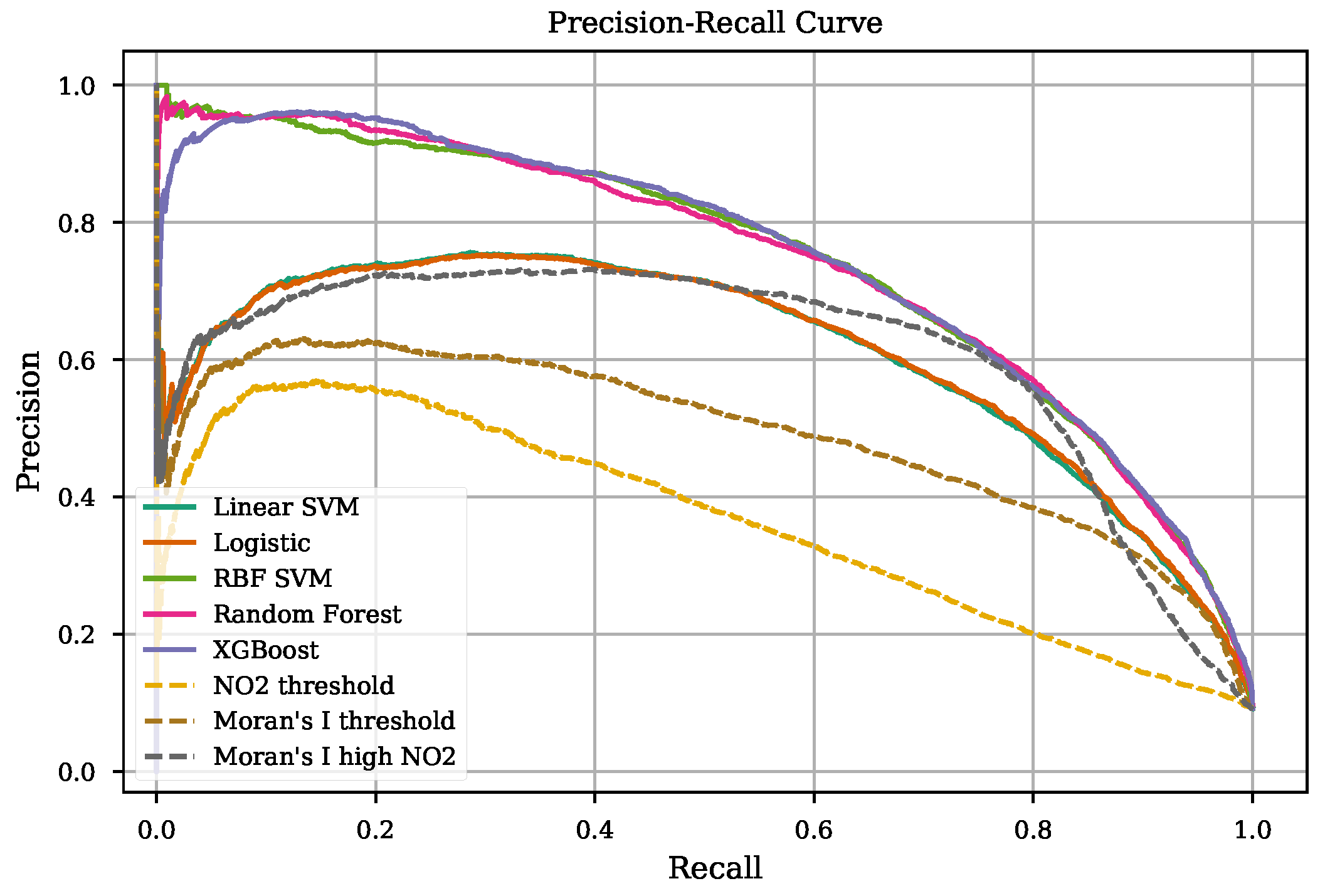
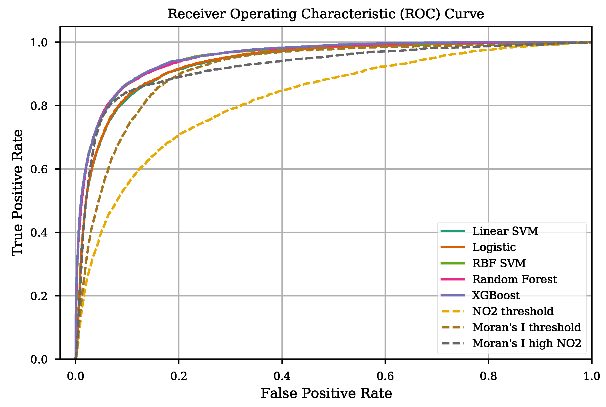
| Model | AP | ROC-AUC |
|---|---|---|
| Linear SVM | 0.609 ± 0.063 | 0.935 ± 0.009 |
| Logistic | 0.610 ± 0.064 | 0.936 ± 0.010 |
| RBF SVM | 0.742 ± 0.031 | 0.951 ± 0.008 |
| Random Forest | 0.743 ± 0.030 | 0.952 ± 0.008 |
| XGBoost | 0.745 ± 0.030 | 0.953 ± 0.007 |
| threshold | 0.375 ± 0.062 | 0.823 ± 0.017 |
| Moran’s I threshold | 0.493 ± 0.063 | 0.912 ± 0.011 |
| Moran’s I on high | 0.607 ± 0.056 | 0.922 ± 0.010 |
| Segmentation Method | Pearson Correlation | Number of Detected Plumes |
|---|---|---|
| XGBoost | 0.834 | 371 |
| Manual Labeling | 0.781 | 334 |
| Random Forest | 0.775 | 436 |
| 0.774 | 334 | |
| Logistic | 0.766 | 452 |
| Linear SVM | 0.765 | 452 |
| RBF SVM | 0.757 | 447 |
| Moran’s I on high | 0.733 | 422 |
| Moran’s I | 0.681 | 448 |
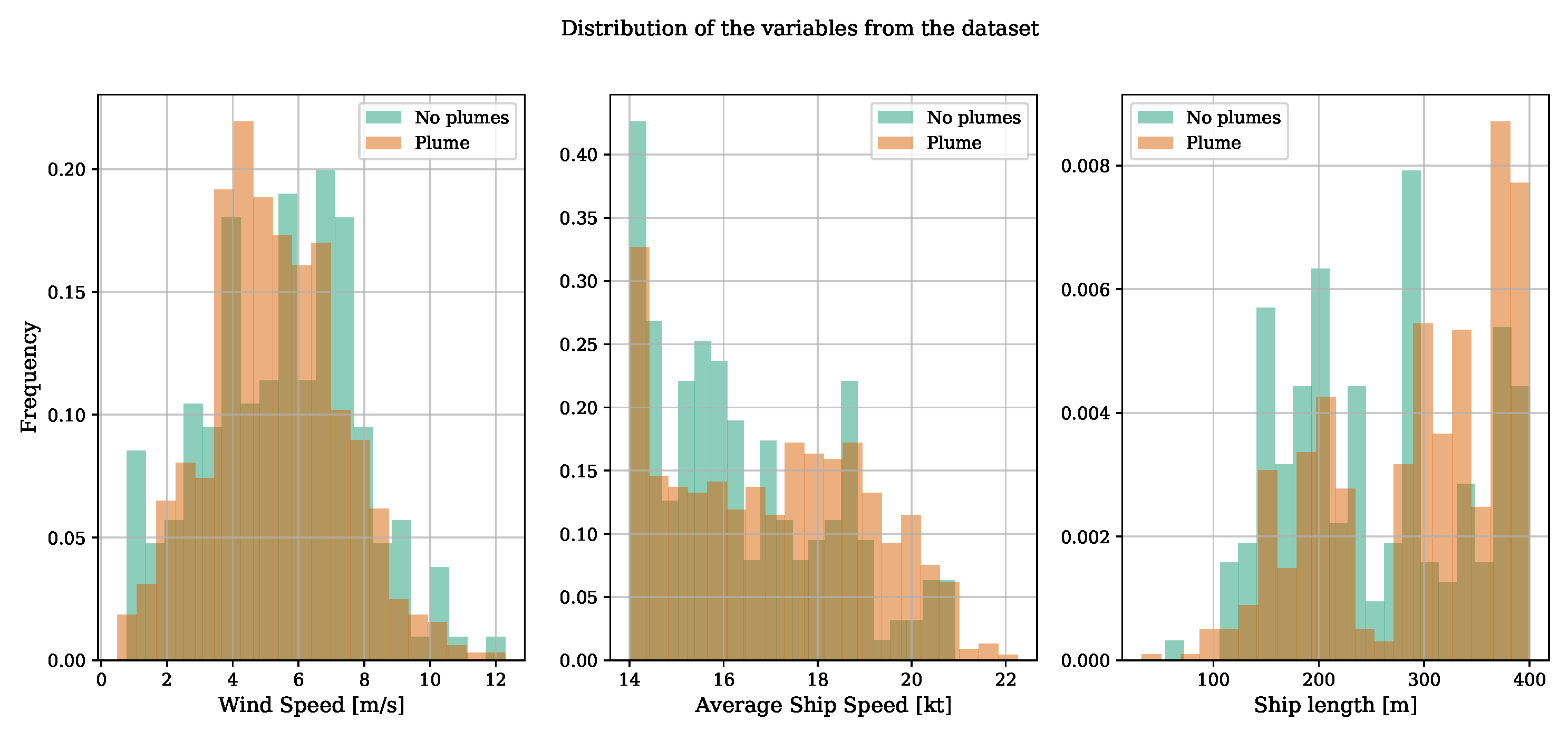
| Variable Name | No Plume Image | Image with a Plume |
|---|---|---|
| Wind speed (m/s) | 5.47 ± 2.31 | 5.27 ± 2.00 |
| Ship speed (kt) | 16.83 ± 2.01 | 17.41 ± 2.04 |
| Ship length (m) | 279.92 ± 86.64 | 303.99 ± 82.79 |
Publisher’s Note: MDPI stays neutral with regard to jurisdictional claims in published maps and institutional affiliations. |
© 2022 by the authors. Licensee MDPI, Basel, Switzerland. This article is an open access article distributed under the terms and conditions of the Creative Commons Attribution (CC BY) license (https://creativecommons.org/licenses/by/4.0/).
Share and Cite
Kurchaba, S.; van Vliet, J.; Verbeek, F.J.; Meulman, J.J.; Veenman, C.J. Supervised Segmentation of NO2 Plumes from Individual Ships Using TROPOMI Satellite Data. Remote Sens. 2022, 14, 5809. https://doi.org/10.3390/rs14225809
Kurchaba S, van Vliet J, Verbeek FJ, Meulman JJ, Veenman CJ. Supervised Segmentation of NO2 Plumes from Individual Ships Using TROPOMI Satellite Data. Remote Sensing. 2022; 14(22):5809. https://doi.org/10.3390/rs14225809
Chicago/Turabian StyleKurchaba, Solomiia, Jasper van Vliet, Fons J. Verbeek, Jacqueline J. Meulman, and Cor J. Veenman. 2022. "Supervised Segmentation of NO2 Plumes from Individual Ships Using TROPOMI Satellite Data" Remote Sensing 14, no. 22: 5809. https://doi.org/10.3390/rs14225809
APA StyleKurchaba, S., van Vliet, J., Verbeek, F. J., Meulman, J. J., & Veenman, C. J. (2022). Supervised Segmentation of NO2 Plumes from Individual Ships Using TROPOMI Satellite Data. Remote Sensing, 14(22), 5809. https://doi.org/10.3390/rs14225809