A Multibranch Crossover Feature Attention Network for Hyperspectral Image Classification

Abstract

Recently, hyperspectral image (HSI) classification methods based on convolutional neural networks (CNN) have shown impressive performance. However, HSI classification still faces two challenging problems: the first challenge is that most existing classification approaches only focus on exploiting the fixed-scale convolutional kernels to extract spectral–spatial features, which leads to underutilization of information; the second challenge is that HSI contains a large amount of redundant information and noise, to a certain extent, which influences the classification performance of CNN. In order to tackle the above problems, this article proposes a multibranch crossover feature attention network (MCFANet) for HSI classification. The MCFANet involves two primary submodules: a cross feature extraction module (CFEM) and rearranged attention module (RAM). The former is devised to capture joint spectral–spatial features at different convolutional layers, scales and branches, which can increase the diversity and complementarity of spectral–spatial features, while the latter is constructed to spontaneously concentrate on recalibrating spatial-wise and spectral-wise feature responses, meanwhile exploit the shifted cascade operation to rearrange the obtained attention-enhanced features to dispel redundant information and noise, and thus, boost the classification performance. Compared with the state-of-the-art classification methods, massive experiments on four benchmark datasets demonstrate the meliority of our presented method.

1. Introduction

Hyperspectral image (HSI), as an image-spectrum merging technology, combinates subdivisional spectroscopy with imaging technology, which contains abundant spatial distribution information of surface targets and hundreds or even thousands of contiguous narrow spectral bands [1,2]. In terms of recognition and classification, which benefit from luxuriant spatial and spectral features, HSI not only has an inherent preponderance over natural images but also can efficaciously distinguish different land-cover categories and objects. Therefore, HSI plays a crucial role in multifarious fields, such as military defense [3], atmospheric science [4], urban planning [5], vegetation ecology [6,7] and environmental monitoring [8,9]. Among the hyperspectral community, one of the most vibrant research applications is HSI classification. However, HSI classification also faces many formidable challenges, such as extensive redundant spectral information interference, available labeled samples deficiency and high intra-class variability.

Initially, traditional HSI classification methods, such as kernel-based and machine-learning approaches [10,11], are composed of two primary parts: feature extraction and classifier optimization. Representative algorithms are band selection (BS) [12], sparse representation classifier (SRC) [13], multinomial logistic regression (MLR) [14], principal components analysis (PCA) [15] and support vector machine (SVM) [16], which utilize rich spectral features to implement HSI classification. However, the above classification approaches only exploit spectral information and do not take full advantage of spatial information. In order to improve the classification performance, many spectral–spatial-based methods have been developed, which incorporate spatial context information into classifiers. For example, 3D morphological profiles [17] and 3D Gabor filters [18] were designed to obtain spectral–spatial features. Li et al. presented multiple kernel learning (MKL) to excavate spectral and spatial information of HSI [19]. Fang et al. constructed a novel local covariance matrix (CM) representation approach, which can capture the relation of spatial information and different spectral bands of HSI [20]. These conventional classification approaches depend on handcrafted features, which leads to the discriminative features’ insufficient extraction and poor robust ability.

In recent years, with the breakthrough of deep learning, HSI classification methods based on deep learning have demonstrated superior performance [21,22,23,24,25]. Chen et al. first applied a convolution neural network (CNN) to HSI classification [26]. Hu et al. raised a framework based on CNN, which comprised five convolutional layers to perform classification tasks [27]. Zhao et al. utilized a 2D CNN to obtain spatial features and then integrated them with spectral information [28]. In order to capture joint spectral–spatial information, Zou et al. constructed a 3D fully convolutional network, which can further obtain high-level semantic features [29]. In order to obtain promising information, Zhang et al. devised a diverse region-based CNN to extract semantic context-aware information [30]. Ge et al. presented a lower triangular network to fuse spectral and spatial features and thus achieved high-dimension semantic information [31]. Nie et al. proposed a multiscale spectral–spatial deformable network, which employed a spectral–spatial joint network to obtain low-level features composed of spatial and spectral information [32]. An effective and efficient CNN-based spectral partitioning residual network was built, which utilized cascaded parallel improved residual blocks to achieve spatial and spectral information [33]. A dual-path siamese CNN was designed by Huang et al., which integrated extended morphological profiles and siamese network with spectral–spatial feature fusion [34]. In order to obtain more prominent spectral–spatial information, Gao et al. designed a multiscale feature extraction module [35]. Shi et al. devised densely connected 3D convolutional layers to capture preliminary spectral–spectral features [36]. Chan et al. utilized spatial and spectral information to train a novel framework for classification [37].

The attention mechanism plays a crucial part in the HSI classification task and focuses on significant information related to the classification task [38,39,40,41,42]. Zhu et al. proposed a spatial attention block to adaptively choose a useful spatial context and a spectral attention block to emphasize necessary spectral bands [43]. In order to optimize and refine the obtained feature maps, Li et al. built a spatial attention block and a channel attention block [44]. Gao et al. proposed a channel–spectral–spatial attention block to enhance the important information and lessen unnecessary ones [45]. Xiong et al. utilized the dynamic routing between attention initiation modules to learn the proposed architecture adaptively [46]. Xi et al. constructed a hybrid residual attention module to enhance vital spatial-spectral information and suppress unimportant ones [47].

Inspired by the above successful classification methods, this article proposes a multibranch crossover feature attention network (MCFANet) for HSI classification. The MCFANet is composed of two primary submodules: a crossover feature extraction module (CFEM) and rearranged attention module (RAM). CFEM is designed to capture spectral–spatial features at different convolutional layers, scales and branches, which can boost the discriminative representations of HSI. Specifically speaking, CFEM consists of three parallel branches with multiple available, receptive fields, which can increase the diversity of spectral–spatial features. Each branch utilizes three additive link units (ALUs) to extract spectral and spatial information while introducing the cross transmission into ALU to take full advantage of spectral–spatial feature flows between different branches. Moreover, each branch also employs dense connections to combinate shallow and deep information and achieve strong related and complementary features for classification. RAM, including a spatial attention branch and a spectral attention branch, is constructed to not only adaptively pay attention to recalibrating spatial-wise and spectral-wise feature responses but also exploit the shifted cascade operation to rearrange the obtained attention-enhanced features to dispel redundant information and noise and, thus, enhance the classification accuracy. The main contributions of this article can be summarized as follows:

(1)

In order to decrease training parameters and accelerate model convergence, we designed an additive link unit (ALU) to replace the conventional 3D convolutional layer. For one, ALU utilizes the spectral feature extraction factor and spatial feature extraction factor to capture joint spectral–spatial features; for another, it also introduces the cross transmission to take full advantage of spectral–spatial feature flows between different branches;

(2)

In order to tackle the fixed-scale convolutional kernels that are difficult to sufficiently extract spectral–spatial features, a crossover feature extraction module (CFEM) was constructed, which can obtain spectral–spatial features at different convolutional scales and branches. CFEM not only utilizes three parallel branches with multiple available, receptive fields to increase the diversity of spectral–spatial features but also applies the dense connection to each branch to incorporate shallow and deep features and, thus, realize robust complementary features for classification;

(3)

In order to dispel the interference of redundant information and noise, we devised a rearranged attention module (RAM) to adaptively concentrate on recalibrating spatial-wise and spectral-wise feature response while exploiting the shifted cascade operation to realign the obtained attention-enhanced features, which are beneficial to boost the classification performance.

The remaining part of this article can be summarized as follows: Section 2 describes in detail our developed MCFANet, Section 3 provides experimental results and discussion and Section 4 gives the conclusion part of this article.

2. Methodology

The proposed MCFANet comprises two significant submodules: crossover feature extraction module (CFEM) and rearranged attention module (RAM), as shown in Figure 1. The former utilizes a multibranch intersection dense connection structure to enhance the representation ability of multiscale spectral–spatial information. The latter can not only focus on adaptively reweighting the significance of spectral-wise and spatial-wise features but also introduce the shifted cascade operation to replume the obtained attention-enhanced features to achieve more discriminative spectral–spatial features while dispelling redundant information and noise, thus, improving the classification performance.

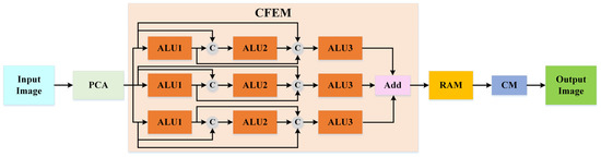
Figure 1. The overall architecture of the developed MCFANet model.

2.1. Additive Link Unit

Generally, low-level features are more concrete and include more spatial details without discrimination, while high-level features are more abstract and contain more semantic information but without a high resolution. In recent years, many studies have indicated that integrating features of different layers is helpful for HSI classification. Zhang et al. designed a deep feature aggregation network to exploit the low-, middle- and high-level features in HSI [48]. Li et al. constructed a multi-attention fusion network to obtain complementary information from different levels [49]. Ge et al. adopted the early fusion method to aggregate features from the front and middle parts of the network and then utilized the fused features to further learn high-level semantic features [31]. Inspired by the above research, we devised an innovative additive link unit (ALU), which introduces the cross transmission to integrate spectral–spatial features of different scales and branches and strengthens spectral–spatial feature representation ability. The structure of the proposed ALU is shown in Figure 2.

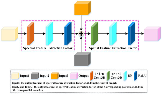
Figure 2. The structure diagram of additive link unit (ALU).

As exhibited in Figure 2, the ALU can be partitioned into three parts: spectral feature extraction factor, cross transmission and spatial feature extraction factor. In order to reduce the training parameters, we utilized the spectral feature extraction factor and spatial feature extraction factor instead of the 3D conventional convolution layer. The spectral feature extraction factor was devised to obtain spectral information, including $1\times 1\times n$ convolution operation, BN layer and Relu activation function. The spatial feature extraction factor was designed to capture spatial information, including $n\times n\times 1$ convolution operation, BN layer and Relu activation function, where $n$ represents the convolution kernel size, BN layer and Relu activation function are used to accelerate the network regularization. In addition, considering that if the three branches are independent of each other, it is difficult to exchange and fuse features at different scales. Therefore, we introduced cross transmission between the spectral feature extraction factor and spatial feature extraction factor to make it easier to achieve feature exchange at different scales and branches, thus improving the richness of spectral–spatial information. It can be calculated as follows:

$$s=\delta (w_0\ast X)$$

(1)

$$z=s+s_1+s_2$$

(2)

$$y=\delta (w_1\ast z)$$

(3)

where $X$ represents the input features of ALU; $s$, $s_1$ and $s_2$ represents the output features of spectral feature extraction factor of ALU at the same position on three branches; $z$ represents the intermediate fusion features; and $y$ represents the output features of ALU. $w_0$ and $w_1$ are the weights of spectral feature extraction factor and spatial feature extraction factor, respectively. $\delta$ is ReLU activation function.

2.2. Crossover Feature Extraction Module

Compared with single-scale feature extraction, integrating spectral–spatial information at different scales is a crucial method for enhancing HSI classification performance. Gao et al. employed mixed depthwise convolution to extract features at different scales from each feature map [50]. Xue et al. built a hierarchical residual network to capture multiscale spectral and spatial features [51]. Nie designed a multiscale spectral–spatial deformable network for HSI classification [32]. DenseNet enabled each layer to receive raw information generated by preceding layers, which was effective for the exploration of new features [52]. Inspired by the aforesaid advantages of approaches, we raised a crossover feature extraction module (CFEM), which not only adopts the multiple available, receptive fields to enrich the diversity of spectral–spatial features but also utilizes cross transmission and dense connection to explore deeper and newer features that are more conducive to HSI classification.

First, CFEM is composed of three parallel branches, and each branch contains three ALUs with diverse convolution kernels to obtain different scale spectral and spatial features of the input image, involving $1\times 1\times 3$, $3\times 3\times 1$, $1\times 1\times 5$, $5\times 5\times 1$, $1\times 1\times 7$ and $7\times 7\times 1$. The structure of each branch is shown in Figure 3. Second, the cross transmission of ALU in each branch can maximize the use of local feature flows between different scales and branches. Furthermore, to increase the complementarity of spectral–spatial features, we applied the dense connection to three ALUs at the same branch. Finally, feature information of different scales and branches was fused by element-wise addition, which can be expressed as follows:

$$\begin{array}{r}Y=add(H(X_0,X_1,\dots ,X_{i-1}),\\ H_1(X_0,X_1,\dots ,X_{i-1}),\\ H_2(X_0,X_1,\dots ,X_{i-1}))\end{array}$$

(4)

where $Y$ denotes the output features of CFEM; $add(·)$ denotes the element-wise summation; $X$ denotes the output features after fusion; and $H_1(·)$, $H_2(·)$ and $H_3(·)$ denote the output features of each branch.

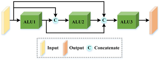
Figure 3. The structure diagram of each branch of cross feature extraction module (CFEM).

2.3. Rearranged Attention Module

The attention mechanism showed unexceptionable potential in boosting the model performance, which can focus on the information related to the current task and suppress ones. Common attention mechanisms can be divided into two categories: spectral attention mechanism and spatial attention mechanism. The former is to seek which feature map is important to learn and redistribute the weight to different channels, while the latter is to identify which area is worth paying attention to and redistribute the weight to the spatial content. Inspired by the above ideas, we designed a rearranged attention module (RAM). RAM concentrates on adaptively recalibrating spatial-wise and spectral-wise responses to obtain attention-enhanced features. Additionally, RAM utilizes the shifted cascade operation to realign the obtained attention-enhanced features to achieve more discriminative features for HSI classification while dispelling redundant information and noise, thus, promoting classification accuracy. The structure of our proposed RAM is exhibited in Figure 4.

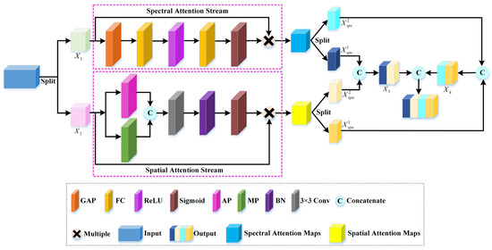
Figure 4. The structure diagram of rearranged attention module (RAM).

As shown in Figure 4, the input feature maps of RAM are indicated by $X\in R^{H\times W\times C}$, where $H$ and $W$ are the height and width of the spatial domain, and $C$ is the spectral band number. We divided the input feature maps $X$ into two sets: $X_1\in R^{H\times W\times (C/2)}$ and $X_2\in R^{H\times W\times (C/2)}$, and transmitted them to the spectral attention branch and spatial branch attention, respectively. In the spectral attention branch, first, we adopted the global average pooling layer (GAP) to transform $X_1\in R^{H\times W\times (C/2)}$ to $X_1\in R^{1\times 1\times (C/2)}$. Then, a simple squeeze-and-excitation mechanism, including two fully connected layers (FCs) with different activation functions, was utilized to calculate the weights of each spectral band and obtain the spectral-wise dependencies $F_{spe}$. Finally, the input feature maps $X_1$ were multiplied by the channel weights $F_{spe}$ to obtain the spectral attention-enhanced output feature maps $X_{spe}$, which can be expressed as follows:

$$\begin{array}{ll}{F}_{spe}& =F{C}_1(F{C}_0(GAP(X_1)))\\ & =\sigma (w_1\ast \delta (w_0\ast GAP(X_1)))\end{array}$$

(5)

$$X_{spe}=X_1\otimes F_{spe}$$

(6)

where $w_0$ and $w_1$ represent the weight matrices of two FCs, respectively; $\delta$ represents the ReLU activation function; and $\sigma$ represents the sigmoid activation function.

In the spatial attention branch, first, we used an average pooling layer (AP) and max pooling layer (MP) to transform $X_2\in R^{H\times W\times (C/2)}$ to $X_2\in R^{H\times W\times 1}$. Second, a concatenation operation was utilized to aggregate the average pooling feature and max pooling feature. Then, the aggregated features were sent to a $3\times 3$ convolution layer to calculate the weights of the spatial domain and obtain the spatial-wise dependencies $F_{spa}$. Finally, the input feature maps $X_2$ were multiplied by the spatial weights $F_{spa}$ to obtain the spatial attention-enhanced output feature maps $X_{spa}$. It can be expressed as follows:

$$F_{spa}=Conv(Concate[AP(X_2),MP(X_2)])$$

(7)

$$X_{spa}=X_2\otimes F_{spa}$$

(8)

Although the outputs of two branches make use of the desired spectral and spatial features, these features are processed over the same feature space, which may impede the information flow. Therefore, we introduce the shifted cascade operation to alleviate this problem. First, we divided the spectral attention-enhanced feature maps $X_{spe}$ and spatial attention-enhanced feature maps $X_{spa}$ into two sunsets, respectively, denoted $X_{spe}^i\in R^{H\times W\times (C/2)},i\in \{1,2\}$, $X_{spa}^j\in R^{H\times W\times (C/2)},j\in \{1,2\}$. Then, the shifted cascade operation was utilized to combine $X_{spe}^1$ with $X_{spa}^2$, and $X_{spe}^2$ with $X_{spa}^1$ to explore the new mixed features $X_3$ and $X_4$. Finally, for $X_3$ and $X_4$, we integrated them by the shifted cascade operation to obtain more conspicuous and representative features $F$ for improving the classification performance. It can be expressed as follows:

$$X_1=Concate[X_{spe}^1,X_{spa}^2]$$

(9)

$$X_2=Concate[X_{spe}^2,X_{spa}^1]$$

(10)

$$F=Concate[X_3,X_4]$$

(11)

where $Concate[]$ denotes the shifted cascade operation, which can explore some new features in other ways and enhance spectral–spatial feature representation ability.

2.4. Framework of the Proposed MCFANet

We utilized the Indian Pines dataset as an example to illustrate the developed method, as shown in Figure 5. First, HSI contains hundreds of spectral bands, and they are highly correlated with each other, leading to the existence of redundant information that is not conducive to the classification task. Therefore, we performed PCA on the raw HSI to eliminate unnecessary information and maintain 20 spectral bands that include the most important features. Second, to fully exploit the property of HSI containing both spectral and spatial data, we extracted a 3D image cube denoted by $X\in R^{11\times 11\times 20}$ as the input of our proposed MCFANet, where $11\times 11$ is the spatial size and 20 is the number of spectral bands. Third, the input data were fed into CFEM comprising three parallel branches to capture multiscale spectral–spatial features and explore deeper and newer features for classification. The branch1 uses three ALUs, which are built by the kernel size of $1\times 1\times 3\times 16$ and $3\times 3\times 1\times 16$ in series, to excavate spectral and spatial features, respectively. Three ALUs were linked to each other by dense connection. Similarly, branch2 uses three ALUs which are built by the kernel size of $1\times 1\times 5\times 16$ and $5\times 5\times 1\times 16$ in series, to excavate spectral and spatial features, respectively. Three ALUs are linked to each other by dense connection. Branch3 uses three ALUs, which are built by the kernel size of $1\times 1\times 7\times 16$ and $7\times 7\times 1\times 16$ to excavate spectral and spatial features, respectively. Three ALUs were linked to each other by dense connection. Then, we adopted the element-wise addition to integrate the output features of three branches and acquire multiscale spectral–spatial features with the size of $11\times 11\times 16$. Next, the multiscale spectral–spatial features were sent to RAM to adaptively recalibrate spatial-wise and spectral-wise responses to obtain spectral attention-enhanced features with the size of $11\times 11\times 8$ and spatial attention-enhanced features with the size of $11\times 11\times 8$. Furthermore, we adopted the shifted cascade operation to rearrange the obtained attention-enhanced features to achieve more discriminative features with the size of $11\times 11\times 16$ for HSI classification. Finally, by using global average pooling, two FC layers and two dropout layers were used to convert the feature maps into a one-dimensional matrix, and class labels were generated via the softmax function.

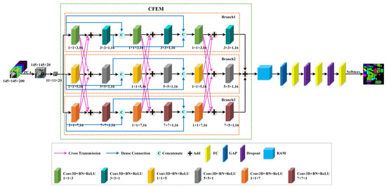
Figure 5. Overall network model.

3. Experimental Results and Discussion

This section introduces in detail the benchmark datasets used, the experimental setup, a series of parameter analyses, and the discussion of experimental results.

3.1. Datasets Description

The Pavia University (UP) dataset was gathered by the Reflective Optics Spectrographic Imaging System (ROSIS-03) sensor in 2003 during a flight campaign in Pavia, Northern Italy. The wavelength range is 0.43–0.86 μm. This dataset contained nine ground truth categories and has 610 × 340 pixels with a spatial resolution of 1.3 m. After excluding 12 bands due to noise, the remaining 103 bands are generally utilized for the experiment.

The Indian Pines (IP) dataset was collected by the airborne visible/infrared imaging spectrometer (AVIRIS) in 1992 in northwestern Indiana, USA. The wavelength range is 0.4–2.5 μm. This dataset contains 16 ground truth categories and has 145 × 145 pixels with a spatial resolution of 20 m. Since 20 bands cannot be reflected by water, the remaining 200 bands are generally utilized for the experiment.

The Salinas Valley (SA) dataset was captured by an AVIRIS sensor in 2011 for the Salinas Valley in California, USA. The wavelength range is 0.36–2.5 μm. This dataset contains 16 ground truth categories and has 512 × 217 pixels with a spatial resolution of 3.7 m. After eliminating bands that cannot be reflected by water, the remaining 204 bands are generally utilized for the experiment.

For the UP and SA datasets, we chose at random 10% labeled samples of each category for training and the remaining 90% labeled samples for testing. For the IP dataset, we select at random 20% labeled samples of each category as the training set, and the remaining 80% labeled samples as the testing set. Table 1, Table 2 and Table 3 list the land-over category details, sample numbers of three datasets and corresponding colors of each category.

Table 1. The information on UP dataset, including number of training and test samples.

No.	Color	Class	Train	Test
1		Asphalt	664	5967
2		Meadows	1865	16,784
3		Gravel	210	1889
4		Trees	307	2757
5		Metal sheets	135	1210
6		Bare Soil	503	4526
7		Bitumen	133	1197
8		Bricks	369	3313
9		Shadows	95	852
	Total		4281	38,495

Table 2. The information on IP dataset, including number of training and test samples.

No.	Color	Class	Train	Test
1		Alfalfa	10	36
2		Corn-notill	286	1142
3		Corn-mintill	166	664
4		Corn	48	189
5		Grass-pasture	97	386
6		Grass-trees	146	584
7		Grass-pasture-mowed	6	22
8		Hay-windrowed	96	382
9		Oats	4	16
10		Soybean-notill	195	777
11		Soybean-mintill	491	1964
12		Soybean-clean	119	474
13		Wheat	41	164
14		Woods	253	1012
15		Buildings-Grass-Tree	78	308
16		Stone-Steel-Towers	19	74
	Total		2055	8194

Table 3. The information of SA dataset, including number of training and test samples.

No.	Color	Class	Train	Test
1		Broccoli-green-weeds-1	201	2825
2		Broccoli-green-weeds-2	373	3353
3		Fallow	198	1178
4		Fallow-rough-plow	140	154
5		Fallow-smooth	268	2410
6		Stubble-trees	396	3563
7		Celery	358	3221
8		Grapes-untrained	1128	10,143
9		Soil-vineyard-develop	621	5582
10		Corn-senseced-green-weeds	328	2950
11		Lettuce-romaine-4 week	107	961
12		Lettuce-romaine-5 week	193	1734
13		Lettuce-romaine-6 week	92	824
14		Lettuce-romaine-7 week	107	963
15		Vineyard-untrained	727	6541
16		Vineyard-vertical-trellis	181	1626
	Total		5418	48,711

https://www.ehu.eus/ccwintco/index.php/Hyperspectral_Remote_Sensing_Scenes (access on 8 November 2022).

3.2. Experimental Setup

All experiments were conducted on a system with an NVIDIA GeForce RTX 2060 SUPER GPU and 6 GB of RAM. The software environment of the system is TensorFlow 2.3.0, Keras 2.4.3, and Python 3.6.

The batch size was set to 16, and the number of training epochs was set to 200. Moreover, we adopted the RMSprop as an optimizer to update the parameters during the training process, and the learning rate was set to 0.0005. Three evaluation indices were used to evaluate the classification performance, i.e., Kappa coefficient (Kappa), average accuracy (AA) and overall accuracy (OA). The Kappa measures the consistency between the ground truth and the classification results. The AA represents the ratio between the total sample numbers of each category and the correctly classified sample numbers. The OA is the proportion of correctly classified samples in the total samples. In theory, the closer these evaluation indices utilized in this article are to 1, the better the classification performance will be.

3.3. Parameter Analysis

In this section, we mainly discussed five vital parameters that impact the classification results of our proposed MCFANet, i.e., the spatial sizes, training sample ratios, principal component numbers, the convolution kernel numbers in additive link unit and the number of additive link units. All experiments used the control variable method to analyze the influence of the aforementioned five important parameters.

3.3.1. Effect of the Spatial Sizes

Different HSI datasets have different feature distributions, and different spatial sizes may generate different classification results. Small size results in insufficient receptive fields, whereas large size results in more noise, which is to the disadvantage of HSI classification. Therefore, we fixed other parameters and set the spatial size to $7\times 7$, $9\times 9$, $11\times 11$, $13\times 13$ and $15\times 15$ to analyze their effects on the classification results of our proposed MCFANet for three datasets. The experimental results are provided in Figure 6. According to Figure 6, for the UP and IP datasets, the optimal spatial size is $11\times 11$. For the SA dataset, as the spatial size is $13\times 13$ and $15\times 15$, three evaluation indices under the two conditions are the same. By considering the number of training parameters and time, the optimal spatial size was set to $13\times 13$ for the SA dataset.

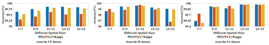
Figure 6. The effect of spatial sizes.

3.3.2. Effect of the Training Sample Ratios

The training sample ratios have a great effect on the HSI classification performance. In order to evaluate the robustness and generalization of the proposed MCFANet, we randomly choose 1%, 3%, 5%, 7%, 10%, 20% and 30% labeled samples for training and the remaining labeled samples for testing. The experimental results are provided in Figure 7. According to Figure 7, for three experimental datasets, it can be seen that as the training sample ratio is 1%, three evaluation indices are the lowest. With the increase in training sample ratios, three evaluation indices gradually improve. For the UP and SA datasets, as the training sample ratio is 10%, three evaluation indices reach a relatively stable level. For the IP dataset, as the training sample ratio is 20%, three evaluation indices reach a relatively stable level. This is because the UP and SA datasets have sufficient labeled samples, so even though the training sample ratio is small, our proposed method can still obtain high classification accuracies. In contrast, the IP dataset contains relatively small labeled samples, which means that the training ratio needs to be large for the proposed method to achieve good classification results. Therefore, the best training sample ratio for the UP and SA datasets is 10%, and the best training sample ratio for the IP dataset is 20%.

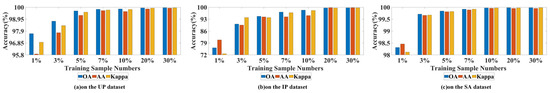
Figure 7. The effect of training sample proportions.

3.3.3. Effect of the Principal Component Numbers

HSI contains hundreds of spectral bands, and they are highly correlated with each other, leading to the existence of redundant information that is not conducive to the classification task. We performed PCA on the raw HSI dataset to reduce the training parameters of the proposed method by reducing the number of spectral bands of the original HSI dataset. We set the number of principal components to 5, 10, 20, 30 and 40 to evaluate their effects on the classification results of our proposed MCFANet for three datasets. The experimental results are provided in Figure 8. According to Figure 8, for the IP and SA datasets, as the number of the principal components is 20, three evaluation indices are obviously superior to other conditions. For the UP dataset, as the principal components numbers are 20, three evaluation indices are 99.82%, 99.62% and 99.80%. As the number of principal components is 40, three evaluation indices are 99.87%, 99.63% and 99.83%. Although the three evaluation indices of the former are 0.05%, 0.01% and 0.03% lower than those of the latter, in contrast, the former needs fewer training parameters and training time. Therefore, the optimal number of principal components for three datasets is 20.

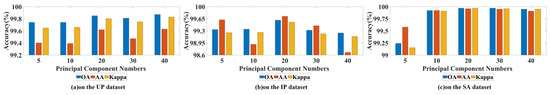
Figure 8. The effect of principal component numbers.

3.3.4. Effect of the Number of Convolutional Kernels in Additive Link Units

The ALU is composed of a spatial feature extraction factor and a spectral feature extraction factor, which are similar to traditional 3D convolutional operations. Therefore, the number of output feature maps of ALU directly impacts the complexity and classification performance of the proposed method. We set the number of convolutional kernels in ALU to 2, 4, 8, 16, 32 and 64 to evaluate their effects on the classification results for three datasets. The experimental results are provided in Figure 9. According to Figure 9, for three datasets, it is clear that as the convolutional kernel number is 16, three evaluation indices are the most advantageous, and the proposed method has the best classification performance. Hence, the optimal number of convolutional kernels for three datasets is 16.

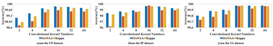
Figure 9. The effect of convolutional kernel numbers in ALU.

3.3.5. Effect of the Number of Additive Link Units

Our proposed MCFANet is composed of three parallel branches, and each branch includes multiple ALUS. A small amount of ALU leads to insufficient feature extraction, whereas too many ALUs lead to cause problems such as overfitting, a more complex structure of the model and gradient explosion, which are not conducive to HSI classification. Therefore, we set the number of ALUs to 2, 3, 4 and 5 to evaluate their effects on the classification results of our proposed MCFANet for three datasets. The experimental results are provided in Figure 10. According to Figure 10, the optimal number of ALUs for UP and SA datasets is 3. For the IP dataset, as the number of ALUs is 3, three evaluation indices are 99.61%, 99.72% and 99.55%. As the number of ALUs is 5, three evaluation indices are 99.68%, 99.69% and 99.64%. Although the OA and Kappa of the former are 0.07% and 0.09% lower than those of the latter, in contrast, the former needs fewer training parameters and training time. All things considered, the optimal number of ALUs for the IP dataset is 3.

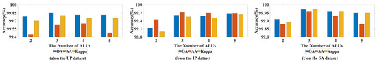
Figure 10. The effect of ALU numbers.

3.4. Ablation Study

Our presented MCFANet involves two submodules: CFEM and RAM. In order to more comprehensively prove the validity of each module, ablation studies were implemented on three benchmark datasets, i.e., not using CFEM (named Netwok1), not using RAM (named Network 2) and using the combination CFEM and RAM (named Network 3). The experimental results are provided in Figure 11. From Figure 11, it is clear that Network 1 has the worst classification accuracies. For example, for the IP dataset, three evaluation indices are 2.37%, 3.13% and 3.05% lower than those of Network 3. In contrast, the classification performance of Network 2 has remarkable improvement. For example, for the UP dataset, three evaluation indices of Network 2 are 2.02%, 3.94% and 2.69% higher than those of Network 1. By comparison, Network 3 has superior classification results, which indicates that our devised CFEM has a greater effect on the classification performance of the presented model, and RAM can further enhance the classification results.

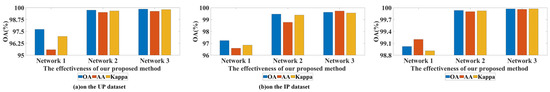
Figure 11. The classification results of ablation study.

3.5. Comparison Methods Discussion

In order to verify the performance of our presented MCFANet, we utilized eleven classical methods for comparison experiments, which can be divided into two categories. One is based on traditional machine learning: SVM, RF, KNN and GuassianNB, which take all spectral bands as input. Another is based on deep learning: spectral–spatial residual network (SSRN) [53] is a 3D CNN, which uses spatial and spectral residual blocks to capture spectral–spatial features; fast, dense spectral–spatial convolution network (FDSSC) [54] utilizes different 3D convolutional kernel sizes based on dense connection to extract spatial and spectral features separately; HybridSN [55] combines one 2D convolutional layer and three 3D convolutional layers; Hybrid 3D/2D CNN (3D_2D_CNN) [56] is similar to HybridSN, which splices together 2D CNN components with 3D CNN components; multibranch 3D-dense attention network (MBDA) [57] exploits 3D CNNs to obtain spectral–spatial information and designs spatial attention mechanisms to enhance the spatial feature representations; multiscale residual network (MSRN) [50] constructs a multiscale residual block with mixed depthwise convolution to achieve multiscale feature learning. Table 4, Table 5 and Table 6 provide the classification results of different methods on three experimental datasets.

Table 4. The classification accuracies of comparison approaches on the UP dataset.

No.	SVM	RF	KNN	GuassianNB	SSRN	FDSSC	2D_3D_CNN	HybridSN	MBDA	MSRN	MCFANet
1	76.52	91.60	89.71	96.50	99.67	98.38	97.98	98.78	99.62	98.99	99.88
2	80.59	89.08	86.46	79.14	98.89	99.77	99.29	99.97	99.83	99.94	99.94
3	81.03	80.01	68.51	30.41	96.30	85.04	97.39	93.30	100.00	99.46	99.95
4	95.85	93.32	96.33	44.02	99.72	100.00	99.47	96.55	98.99	93.16	99.53
5	99.59	99.33	99.66	79.47	99.92	100.00	99.77	95.92	99.76	40.58	99.51
6	94.25	88.88	82.82	39.15	99.72	99.36	98.85	99.96	100.00	100.00	99.91
7	0.00	84.70	76.32	38.91	85.39	100.00	96.81	97.15	100.00	33.78	99.92
8	64.73	79.05	77.29	70.03	96.07	99.97	93.83	91.51	99.26	91.38	99.67
9	99.88	100.00	100.00	100.00	96.15	100.00	99.33	99.25	95.15	74.98	99.29
OA	80.21	88.84	86.01	65.87	98.23	98.71	98.42	98.23	99.61	87.22	99.85
AA	66.47	85.35	82.34	72.57	97.89	98.29	97.43	95.80	99.15	88.86	99.62
Kappa×100	72.39	84.93	81.05	56.61	97.70	98.29	97.90	97.65	99.48	83.38	99.80
FLOPs (×106)	-	-	-	-	1.39	0.51	0.51	10.24	0.48	0.32	1.13
Test Time (s)	-	-	-	-	9.33	11.89	0.87	10.32	10.86	10.88	17.82

Table 5. The classification accuracies of comparison approaches on the IP dataset.

No.	SVM	RF	KNN	GuassianNB	SSRN	FDSSC	2D_3D_CNN	HybridSN	MBDA	MSRN	MCFANet
1	0.00	83.33	11.76	42.50	100.00	0.00	97.62	90.91	97.62	86.36	94.74
2	61.21	72.33	48.73	40.95	94.98	95.38	88.17	97.04	97.09	91.27	99.56
3	78.31	79.57	56.67	23.28	97.16	96.10	87.61	99.46	98.42	96.98	99.85
4	81.82	73.33	52.59	9.04	89.77	100.00	87.80	98.20	100.00	100.00	100.00
5	93.58	89.01	83.33	2.75	99.06	91.65	94.06	94.53	97.52	95.81	100.00
6	79.09	79.80	77.58	67.59	97.76	99.69	93.92	99.53	99.84	99.22	99.83
7	0.00	100.00	88.33	100.00	100.00	0.00	95.45	85.00	100.00	78.57	100.00
8	84.86	92.10	88.32	83.13	100.00	91.10	97.50	96.41	100.00	100.00	100.00
9	0.00	0.00	50.00	11.11	66.67	0.00	100.00	100.00	100.00	100.00	100.00
10	72.83	99.37	65.23	23.34	97.63	99.76	90.85	99.40	100.00	98.28	99.36
11	56.77	75.59	70.69	63.73	94.48	99.41	90.73	99.05	99.45	99.95	99.49
12	45.48	59.96	64.46	15.79	96.64	93.84	90.93	89.43	90.81	94.14	99.57
13	87.43	91.95	80.30	87.92	98.92	98.92	80.53	98.40	100.00	100.00	98.80
14	85.90	90.69	91.85	75.14	97.70	99.65	98.75	96.67	98.44	98.87	100.00
15	81.82	76.40	59.86	62.71	89.38	99.14	92.43	98.79	99.71	99.71	100.00
16	98.46	98.46	98.48	100.00	100.00	97.53	94.12	94.05	80.61	85.42	94.87
OA	68.89	79.00	69.45	47.84	96.04	97.45	91.65	97.45	98.21	97.27	99.61
AA	53.09	67.73	61.98	50.53	93.42	79.61	85.30	92.52	96.58	92.80	99.72
Kappa × 100	63.51	75.80	65.01	41.22	95.48	97.09	90.44	97.09	97.96	96.88	99.55
FLOPs (×106)	-	-	-	-	0.17	3.81	0.52	10.24	0.48	0.32	0.80
Test Time (s)	-	—-	-	-	2.23	5.65	0.31	2.43	7.40	0.88	6.52

Table 6. The classification accuracies of comparison approaches on the SA dataset.

No.	SVM	RF	KNN	GuassianNB	SSRN	FDSSC	2D_3D_CNN	HybridSN	MBDA	MSRN	MCFANet
1	100.00	99.89	99.83	99.87	100.00	100.00	100.00	100.00	100.00	100.00	100.00
2	99.08	99.67	99.26	99.53	99.69	100.00	99.92	100.00	100.00	100.00	100.00
3	92.14	95.05	91.06	89.46	99.57	92.60	99.95	100.00	100.00	100.00	100.00
4	97.94	98.57	97.50	97.09	99.24	98.81	97.99	99.77	96.15	90.31	99.92
5	97.87	98.96	98.26	97.28	99.21	99.96	99.41	99.84	100.00	100.00	99.92
6	99.92	99.92	100.00	99.97	100.00	100.00	100.00	100.00	100.00	100.00	100.00
7	98.02	99.57	99.16	97.78	100.00	100.00	99.85	100.00	99.97	100.00	100.00
8	70.12	77.56	72.88	74.36	99.47	99.92	97.36	99.67	99.73	98.31	100.00
9	98.78	98.87	99.09	98.90	100.00	99.58	99.81	100.00	100.00	100.00	100.00
10	87.86	93.91	89.89	59.84	99.13	99.86	98.97	100.00	100.00	97.67	99.90
11	92.96	93.68	91.81	31.16	98.02	96.75	97.00	98.16	95.56	99.31	99.38
12	94.95	96.88	95.14	91.76	99.56	99.89	99.40	100.00	99.89	99.89	100.00
13	92.50	96.83	94.45	94.62	100.00	100.00	98.31	100.00	99.89	100.00	99.88
14	97.45	97.59	96.63	67.90	99.60	100.00	100.00	99.61	95.58	96.69	100.00
15	81.99	78.56	60.28	45.88	84.27	89.34	97.39	99.71	99.83	96.56	100.00
16	98.97	98.81	99.00	85.79	99.82	100.00	100.00	100.00	100.00	99.94	100.00
OA	88.54	91.22	87.29	76.77	97.20	97.93	98.81	99.83	99.63	98.68	99.97
AA	92.60	95.16	93.13	86.26	98.75	98.99	99.11	99.87	99.63	99.04	99.96
Kappa × 100	87.18	90.21	85.85	74.46	96.89	97.70	98.67	99.82	99.58	98.53	99.97
FLOPs (×106)	-	-	-	-	4.15	3.93	0.52	10.24	0.48	0.32	1.13
Test Time (s)	-	-	-	-	16.57	25.81	4.70	15.58	12.69	14.59	30.91

First, as shown in Table 4, Table 5 and Table 6, it can be seen that our developed MCFANet achieves excellent classification performance and has the highest classification accuracies in most categories. For the UP dataset, compared with other methods, the OA, AA and Kappa of the proposed MCFANet have an increase of approximately 0.34–33.98%, 0.47–33.15% and 0.32–43.17%, respectively. For the IP dataset, the OA, AA and Kappa of the proposed MCFANet have an increase of approximately 1.4–51.77%, 3.15–49.19% and 1.5~58.33%, respectively. For the SA dataset, the OA, AA and Kappa of the proposed MCFANet have an increase of approximately 0.14–23.20%, 0.09–13.7% and 0.15–25.51%, respectively. Overall, compared with seven deep learning-based classification approaches, SVM, RF, KNN and GuassianNB have lower classification accuracies, of which GuassianNB performs the worst. This is because they only capture features in the spectral domain and neglect ample spatial features. In addition, they need to rely on the prior information of experienced experts, leading to inferior robustness and generalization ability. Due to the hierarchical structure, seven methods based on deep learning can extract low-, middle- and high-level spectral–spatial features automatically and obtain decent classification accuracies.

Second, MBDA, MSRN and our proposed MCFANet adopted the multiscale feature extraction strategy. MBDA uses three parallel branches with a convolutional kernel with different sizes to capture multiscale spectral–spatial features. MSRN utilizes a multiscale residual block to perform multiscale feature extraction, which is composed of depthwise separable convolution with mixed depthwise convolution. It is clear from Table 4, Table 5 and Table 6 of the three methods that our proposed MCFANet obtains superior classification performance. For the UP dataset, three evaluation indices of the proposed MCFANet are 0.34%, 0.47% and 0.32% higher than those of MBDA and are 12.63%, 10.76% and 16.42% higher than those of MSRN. For the IP dataset, three evaluation indices of the proposed MCFANet are 1.4%, 3.15% and 1.59% higher than those of MBDA and are 2.34%, 6.90% and 2.67% higher than those of MSRN. For the SA dataset, three evaluation indices of the proposed MCFANet are 0.34%, 0.33% and 0.39% higher than those of MBDA and are 1.29%, 0.92% and 1.44% higher than those of MSRN. This is because compared with MBDA and MSRN, our proposed MCFANet can introduce not only multiple available, receptive fields to capture multiscale spectral–spatial features but also utilize dense connection and cross transmission to aggregate spectral–spatial features from different layers and branches.

Third, according to Table 4, Table 5 and Table 6, we also can obviously see that the evaluation indices of MBDA occupy the second place. This is because MBDA builds a spatial attention module to focus on spatial features that are related to HSI classification. Our proposed MCFANet also constructs a RAM to enhance spectral–spatial features and achieve the greatest classification accuracies. These indicate that the attention mechanism can boost classification performance to a certain degree. For the UP dataset, three evaluation indices of the proposed MCFANet are 0.34%, 0.47% and 0.32% higher than those of MBDA. For the IP dataset, three evaluation indices of the proposed MCFANet are 1.4%, 3.15% and 1.59% higher than those of MBDA. For the SA dataset, three evaluation indices of the proposed MCFANet are 0.34%, 0.33% and 0.39% higher than those of MBDA. This is because our designed RAM can not only focus on adaptively reweighting the significance of spectral-wise and spatial-wise features but also introduce the shifted cascade operation to replume the obtained attention-enhanced features to achieve more discriminative spectral–spatial features while dispelling redundant information and noise and thus, improving the classification performance.

Furthermore, as shown in Table 4, Table 5 and Table 6, it is clear that compared with six DL-based classification approaches, the FLOPs and test time of our proposed MCFANet are not the least, which indicates that our presented method still has some shortcomings. This could be because our designed CFEM includes different parallel branches, and the spectral–spatial information between branches is shared with each other; the spectral–spatial features at different scales and branches are effectively integrated, but the structure of our developed model and the test time is relatively large and not superior. Therefore, how to shorten the test time and reduce the complexity of the proposed MCFANet is still a problem worth studying.

Moreover, Figure 12, Figure 13 and Figure 14 provide the classification visual result maps of eleven comparison methods on the three experimental datasets. In contrast, SVM, RF, KNN and GuassianNB have coarse classification maps and contain vast noise and high misclassification rates. The classification maps of SSRN, FDSSC, 3D_2D_CNN, HybridSN, MBAN, MSRN and MCFANet have significantly improved and become clear. By comparison, the classification maps of our developed MCFANet are smoother and more accurate and are highly consistent with the ground-truth map on the three public datasets.

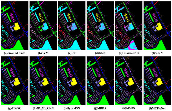
Figure 12. The visual classification maps of diverse approaches on the UP dataset.

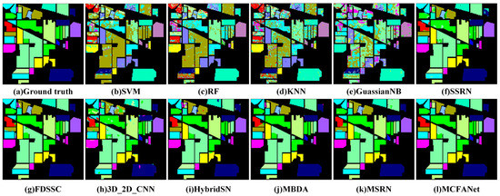
Figure 13. The visual classification maps of diverse approaches on the IP dataset.

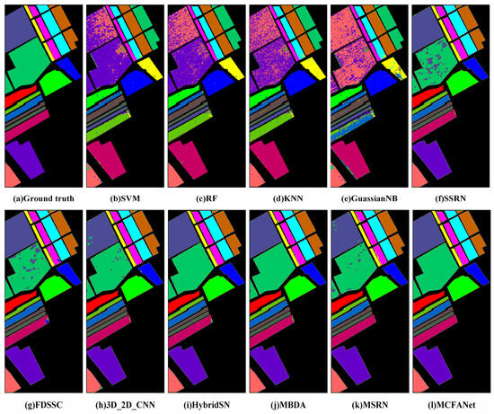
Figure 14. The visual classification maps of diverse approaches on the SA dataset.

4. Conclusions

In this article, we developed a multibranch crossover feature attention network (MCFANet) for HSI classification. The MCFANet includes two main functional submodules: a cross feature extraction module (CFEM) and rearranged attention module (RAM). The former is designed to capture spectral–spatial features at different convolutional layers, scales and branches, which can increase the diversity and complementarity of spectral–spatial information. While the latter is constructed to not only adaptively pay attention to recalibrating spatial-wise and spectral-wise feature responses but also exploit the shifted cascade operation to rearrange the obtained attention-enhanced features to dispel redundant information and noise and, thus, improve the classification accuracy. The experimental results of plentiful comparison experiments and ablation studies demonstrate that our proposed MCFANet obtains superior classification accuracies on three benchmark datasets and has robust generalization ability while it can be extended to other HSI datasets.

Labeling the HSI pixels is expensive and time-consuming, and HSI contains limited labeled samples, therefore in future work, we will apply the semi-supervised or unsupervised classification approaches and data enhancement techniques to HSI classification to deal with the above problem of lack of labeled samples.

References

- Guo, Y.; Chanussot, J.; Jia, X.; Benediktsson, J.A. Multiple Kernel learning for hyperspectral image classification: A review. IEEE Trans. Geosci. Remote Sens. 2017, 55, 6547–6565. [Google Scholar] [CrossRef]
- Li, S.; Song, W.; Fang, L.; Chen, Y.; Ghamisi, P.; Benediktsson, J.A. Deep learning for hyperspectral image classification: An overview. IEEE Trans. Geosci. Remote Sens. 2019, 57, 6690–6709. [Google Scholar] [CrossRef]
- Xu, Y.; Wu, Z.; Chanussot, J.; Wei, Z. Joint reconstruction and anomaly detection from compressive hyperspectral images using mahalanobis distance-regularized tensor RPCA. IEEE Trans. Geosci. Remote Sens. 2018, 56, 2919–2930. [Google Scholar] [CrossRef]
- Pyo, J.; Duan, H.; Ligaray, M.; Kim, M.; Baek, S.; Kwon, Y.S.; Lee, H.; Kang, T.; Kim, K.; Cha, Y.; et al. An integrative remote sensing application of stacked autoencoder for atmospheric correction and cyanobacteria estimation using hyperspectral imagery. Remote Sens. 2020, 12, 1073. [Google Scholar] [CrossRef]
- Ghamisi, P.; Dalla Mura, M.; Benediktsson, J.A. A survey on spectral classification techniques based on attribute profiles. IEEE Trans. Geosci. Remote Sens. 2015, 53, 2335–2353. [Google Scholar] [CrossRef]
- Camps-Valls, G.; Tuia, D.; Bruzzone, L.; Benediktsson, J.A. Advances in hyperspectral image classification: Earth monitoring with statistical learning methods. IEEE Signal Process. Mag. 2014, 31, 45–54. [Google Scholar] [CrossRef]
- Ghiyamat, A.; Shafri, H.Z. A review on hyperspectral remote sensing for homogeneous and heterogeneous forest biodiversity assessment. Int. J. Remote Sens. 2010, 31, 1837–1856. [Google Scholar] [CrossRef]
- Bioucas-Dias, J.M.; Plaza, A.; Camps-Valls, P.; Nasrabadi, N.; Nasrabadi, J. Hyperspectral remote sensing data analysis and future challenges. IEEE Geosci. Remote Sens. Mag. 2013, 1, 6–36. [Google Scholar] [CrossRef]
- Malthus, T.J.; Mumby, P.J. Remote sensing of the coastal zone: An overview and priorities for future research. Int. J. Remote Sens. 2003, 24, 2805–2815. [Google Scholar] [CrossRef]
- Camps-Valls, G.; Bruzzone, L. Kernel-based methods for hyperspectral image classification. IEEE Trans. Geosci. Remote Sens. 2005, 43, 1351–1362. [Google Scholar] [CrossRef]
- Gewali, U.B.; Monteiro, S.T.; Saber, E. Machine learning based hyperspectral image analysis: A survey. arXiv 2018, arXiv:1802.08701. [Google Scholar]
- Du, H.; Qi, H.; Wang, X.; Ramanath, R.; Snyder, W.E. Band selection using independent component analysis for hyperspectral image processing. In Proceedings of the 32nd Applied Imagery Pattern Recognition Workshop, Washington, DC, USA, 15–17 October 2003; pp. 93–98. [Google Scholar]
- Chen, Y.; Nasrabadi, N.M.; Tran, T.D. Hyperspectral image classification via kernel sparse representation. IEEE Trans. Geosci. Remote Sens. 2013, 51, 217–231. [Google Scholar] [CrossRef]
- Li, J.; Bioucas-Dias, J.M.; Plaza, A. Semisupervised hyperspectral image segmentation using multinomial logistic regression with active learning. IEEE Trans. Geosci. Remote Sens. 2010, 48, 4085–4098. [Google Scholar] [CrossRef]
- Kang, X.; Xiang, X.; Li, S.; Benediktsson, J.A. PCA-based edge preserving features for hyperspectral image classification. IEEE Trans. Geosci. Remote Sens. 2017, 55, 7140–7151. [Google Scholar] [CrossRef]
- Mercier, G.; Lennon, M. Support vector machines for hyperspectral image classification with spectral-based kernels. In Proceedings of the 2003 IEEE International Geoscience and Remote Sensing Symposium (IGARSS 2003), Toulouse, France, 21–25 July 2003; Volume 6, pp. 288–290. [Google Scholar]
- Zhu, J.; Hu, J.; Jia, S.; Jia, X.; Li, Q. Multiple 3-D feature fusion framework for hyperspectral image classification. IEEE Trans. Geosci. Remote Sens. 2018, 56, 1873–1886. [Google Scholar] [CrossRef]
- Huo, L.-Z.; Tang, P. Spectral and spatial classification of hyperspectral data using SVMs and Gabor textures. In Proceedings of the 2011 IEEE International Geoscience and Remote Sensing Symposium, IGARSS 2011, Vancouver, BC, Canada, 24–29 July 2011; pp. 1708–1711. [Google Scholar]
- Li, J.; Marpu, P.R.; Plaza, A.; Bioucas-Dias, J.M.; Benediktsson, J.A. Generalized composite kernel framework for hyperspectral image classification. IEEE Trans. Geosci. Remote Sens. 2013, 51, 4816–4829. [Google Scholar] [CrossRef]
- Fang, L.; He, N.; Li, S.; Plaza, A.J.; Plaza, J. A new spatial–spectral feature extraction method for hyperspectral images using local covariance matrix representation. IEEE Trans. Geosci. Remote Sens. 2018, 56, 3534–3546. [Google Scholar] [CrossRef]
- Mou, L.; Zhu, X. Learning to pay attention on spectral domain: A spectral attention module-based convolutional network for hyperspectral image classification. IEEE Trans. Geosci. Remote Sens. 2020, 58, 110–122. [Google Scholar] [CrossRef]
- He, M.; Li, B.; Chen, H. Multi-scale 3d deep convolutional neural network for hyperspectral image classification. In Proceedings of the 2017 IEEE International Conference on Image Processing (ICIP), Beijing, China, 17–20 September 2017; pp. 3904–3908. [Google Scholar]
- Sellami, A.; Farah, M.; Farah, I.R.; Solaiman, B. Hyperspectral imagery classification based on semi-supervised 3-D deep neural network and adaptive band selection. Expert Syst. Appl. 2019, 129, 246–259. [Google Scholar] [CrossRef]
- Haut, J.M.; Paoletti, M.E.; Plaza, J.; Plaza, A.; Li, J. Visual Attention-Driven Hyperspectral Image Classification. IEEE Trans. Geosci. Remote Sens. 2019, 57, 8065–8080. [Google Scholar] [CrossRef]
- Fang, B.; Li, Y.; Zhang, H.; Chan, J.C.W. Hyperspectral Images Classification Based on Dense Convolutional Networks with Spectral-Wise Attention Mechanism. Remote Sens. 2019, 11, 159. [Google Scholar] [CrossRef]
- Chen, Y.; Jiang, H.; Li, C.; Jia, X.; Ghamisi, P. Deep feature extraction and classification of hyperspectral images based on convolutional neural networks. IEEE Trans. Geosci. Remote Sens. 2016, 54, 6232–6251. [Google Scholar] [CrossRef]
- Hu, W.; Huang, Y.; Wei, L.; Zhang, F.; Li, H. Deep convolutional neural networks for hyperspectral image classification. J. Sens. 2015, 2015, 258619. [Google Scholar] [CrossRef]
- Zhao, W.; Du, S. Spectral-spatial feature extraction for hyperspectral image classification: A dimension reduction and deep learning approach. IEEE Trans. Geosci. Remote Sens. 2016, 54, 4544–4554. [Google Scholar] [CrossRef]
- Zou, L.; Zhu, X.; Wu, C.; Liu, Y.; Qu, L. Spectral–Spatial Exploration for Hyperspectral Image Classification via the Fusion of Fully Convolutional Networks. IEEE J. Sel. Top. Appl. Earth Observ. Remote Sens. 2020, 13, 659–674. [Google Scholar] [CrossRef]
- Zhang, M.; Li, W.; Du, Q. Diverse Region-Based CNN for Hyperspectral Image Classification. IEEE Trans. Geosci. Remote Sens. 2018, 27, 2623–2634. [Google Scholar] [CrossRef]
- Ge, Z.; Cao, G.; Zhang, Y.; Li, X.; Shi, H.; Fu, P. Adaptive Hash Attention and Lower Triangular Network for Hyperspectral Image Classification. IEEE Trans. Geosci. Remote Sens. 2022, 59, 5509119. [Google Scholar] [CrossRef]
- Nie, J.; Xu, Q.; Pan, J.; Guo, M. Hyperspectral Image Classification Based on Multiscale Spectral–Spatial Deformable Network. IEEE Geosci. Remote Sens. Lett. 2022, 19, 5500905. [Google Scholar] [CrossRef]
- Zhang, X.; Shang, S.; Tang, X.; Feng, J.; Jiao, L. Spectral Partitioning Residual Network with Spatial Attention Mechanism for Hyperspectral Image Classification. IEEE Trans. Geosci. Remote Sens. 2022, 60, 5507714. [Google Scholar] [CrossRef]
- Huang, L.; Chen, Y. Dual-Path Siamese CNN for Hyperspectral Image Classification with Limited Training Samples. IEEE Geosci. Remote Sens. Lett. 2021, 18, 518–522. [Google Scholar] [CrossRef]
- Gao, H.; Zhang, Y.; Chen, Z.; Li, C. A Multiscale Dual-Branch Feature Fusion and Attention Network for Hyperspectral Images Classification. IEEE J. Sel. Top. Appl. Earth Observ. Remote Sens. 2021, 13, 8180–8192. [Google Scholar] [CrossRef]
- Shi, H.; Cao, G.; Zhnag, Y.; Ge, Z.; Liu, Y.; Fu, P. H2A2Net: A Hybrid Convolution and Hybrid Resolution Network with Double Attention for Hyperspectral Image Classification. Remote Sens. 2022, 14, 4235. [Google Scholar] [CrossRef]
- Chan, R.H.; Li, R. A 3-Stage Spectral-Spatial Method for Hyperspectral Image Classification. Remote Sens. 2022, 14, 3998. [Google Scholar] [CrossRef]
- Wang, Q.; Liu, S.; Chanussot, J.; Li, X. Scene classification with recurrent attention of VHR remote sensing images. IEEE Trans. Geosci. Remote Sens. 2019, 57, 1155–1167. [Google Scholar] [CrossRef]
- Yang, K.; Sun, H.; Zou, C.; Lu, X. Cross-Attention Spectral–Spatial Network for Hyperspectral Image Classification. IEEE Trans. Geosci. Remote Sens. 2022, 60, 5518714. [Google Scholar] [CrossRef]
- Xiang, J.; Wei, C.; Wang, M.; Teng, L. End-to-End Multilevel Hybrid Attention Framework for Hyperspectral Image Classification. IEEE Geosci. Remote Sens. Lett. 2019, 57, 1155–1167. [Google Scholar] [CrossRef]
- Huang, H.; Luo, L.; Pu, C. Self-Supervised Convolutional Neural Network via Spectral Attention Module for Hyperspectral Image Classification. IEEE Geosci. Remote Sens. Lett. 2022, 19, 6006205. [Google Scholar] [CrossRef]
- Tu, B.; He, W.; He, W.; Ou, X.; Plaza, A. Hyperspectral Classification via Global-Local Hierarchical Weighting Fusion Network. IEEE J. Sel. Top. Appl. Earth Observ. Remote Sens. 2021, 15, 182–200. [Google Scholar] [CrossRef]
- Zhu, M.; Jiao, L.; Liu, F.; Yang, F.; Wang, J. Residual Spectral–Spatial Attention Network for Hyperspectral Image Classification. IEEE Trans. Geosci. Remote Sens. 2021, 59, 449–462. [Google Scholar] [CrossRef]
- Li, R.; Zheng, S.; Chen, D.; Yang, Y.; Wang, X. Classification of Hyperspectral Image Based on Double-Branch Dual-Attention Mechanism Network. Remote Sens. 2020, 12, 582. [Google Scholar] [CrossRef]
- Gao, H.; Miao, Y.; Cao, X.; Li, C. Densely Connected Multiscale Attention Network for Hyperspectral Image Classification. IEEE J. Sel. Top. Appl. Earth Observ. Remote Sens. 2021, 14, 2563–2576. [Google Scholar] [CrossRef]
- Xiong, Z.; Yuan, Y.; Wang, Q. AI-NET: Attention inception neural networks for hyperspectral image classification. In Proceedings of the IGARSS 2018—2018 IEEE International Geoscience and Remote Sensing Symposium, Valencia, Spain, 22–27 July 2018; pp. 2647–2650. [Google Scholar]
- Xi, B.; Li, J.; Li, Y.; Song, R.; Shi, Y.; Liu, S.; Du, Q. Deep Prototypical Networks with Hybrid Residual Attention for Hyperspectral Image Classification. IEEE J. Sel. Top. Appl. Earth Observ. Remote Sens. 2020, 13, 3683–3700. [Google Scholar] [CrossRef]
- Zhang, C.; Li, G.; Lei, R.; Du, S.; Zhang, X.; Zheng, H.; Wu, Z. Deep Feature Aggregation Network for Hyperspectral Remote Sensing Image Classification. IEEE J. Sel. Top. Appl. Earth Observ. Remote Sens. 2020, 13, 5314–5325. [Google Scholar] [CrossRef]
- Li, Z.; Zhao, X.; Xu, Y.; Li, W.; Zhai, L.; Fang, Z.; Shi, X. Hyperspectral Image Classification with Multiattention Fusion Network. IEEE Geosci. Remote Sens. Lett. 2022, 19, 5503305. [Google Scholar] [CrossRef]
- Gao, H.; Yang, Y.; Li, C.; Gao, L.; Zhangm, B. Multiscale Residual Network With Mixed Depthwise Convolution for Hyperspectral Image Classification. IEEE Trans. Geosci. Remote Sens. 2021, 59, 3396–3408. [Google Scholar] [CrossRef]
- Xue, X.; Yu, X.; Liu, B.; Tan, X.; Wei, X. HResNetAM: Hierarchical Residual Network With Attention Mechanism for Hyperspectral Image Classification. IEEE J. Sel. Top. Appl. Earth Observ. Remote Sens. 2021, 14, 3566–3580. [Google Scholar] [CrossRef]
- Huang, G.; Liu, Z.; Weinberger, K.Q.; van der Maaten, L. Densely connected convolutional networks. In Proceedings of the 2017 IEEE Conference on Computer Vision and Pattern Recognition (CVPR), Honolulu, HI, USA, 21–26 July 2017; pp. 4700–4708. [Google Scholar]
- Zhong, Z.; Li, J.; Luo, Z.; Chapman, M. Spectral-Spatial Residual Network for Hyperspectral Image Classification: A 3-D Deep Learning Framework. IEEE Trans. Geosci. Remote Sens. 2018, 56, 847–858. [Google Scholar] [CrossRef]
- Wu, W.; Dou, S.; Jiang, Z.; Sun, L. A Fast Dense Spectral-Spatial Convolution Network Framework for Hyperspectral Images Classification. Remote Sens. 2018, 10, 1068. [Google Scholar]
- Kumar Roy, S.; Krishna, G.; Ram Dubey, S.; Chaudhuri, B.B. HybridSN: Exploring 3-D–2-D CNN Feature Hierarchy for Hyperspectral Image Classification. IEEE Geosci. Remote Sens. Lett. 2020, 17, 277–281. [Google Scholar]
- Ahmad, M.; Shabbir, S.; Aamir Raza, P.; Mazzara, M.; Distefano, S.; Mehmood Khan, A. Hyperspectral Image Classification: Artifacts of Dimension Reduction on Hybrid CNN. arXiv 2021, arXiv:2101.10532v. [Google Scholar]
- Yin, J.; Qi, C.; Huang, W.; Chen, Q.; Qu, J. Multibranch 3D-Dense Attention Network for Hyperspectral Image Classification. IEEE Access 2022, 10, 71886–71898. [Google Scholar] [CrossRef]
Publisher’s Note: MDPI stays neutral with regard to jurisdictional claims in published maps and institutional affiliations. |
© 2022 by the authors. Licensee MDPI, Basel, Switzerland. This article is an open access article distributed under the terms and conditions of the Creative Commons Attribution (CC BY) license (https://creativecommons.org/licenses/by/4.0/).