Abstract
Greater adoption and better management of spatially complex, conservation systems such as agroforestry (AF) are dependent on determining methods suitable for delineating in-field variability. However, no work has been conducted using repeated electromagnetic induction (EMI) or apparent electrical conductivity (ECa) surveys in AF systems within the Ozark Highlands of northwest Arkansas. As a result, objectives were to (i) evaluate spatiotemporal ECa variability; (ii) identify ECa-derived soil management zones (SMZs); (iii) establish correlations among ECa survey data and in situ, soil-sensor volumetric water content, sentential site soil-sample EC, and gravimetric water content and pH; and (iv) determine the optimum frequency at which ECa surveys could be conducted to capture temporal changes in field variability. Monthly ECa surveys were conducted between August 2020 and July 2021 at a 4.25 ha AF site in Fayetteville, Arkansas. The overall mean perpendicular geometry (PRP) and horizontal coplanar geometry (HCP) ECa ranged from 1.8 to 18.0 and 3.1 to 25.8 mS m−1, respectively, and the overall mean HCP ECa was 67% greater than the mean PRP ECa. The largest measured ECa values occurred within the local drainage way or areas of potential groundwater movement, and the smallest measured ECa values occurred within areas with decreased effective soil depth and increased coarse fragments. The PRP and HCP mean ECa, standard deviation (SD), and coefficient of variation (CV) were unaffected (p > 0.05) by either the weather or growing/non-growing season. K-means clustering delineated three precision SMZs that were reflective of areas with similar ECa and ECa variability. Results from this study provided valuable information regarding the application of ECa surveys to quantify small-scale changes in soil properties and delineate SMZs in highly variable AF systems.
1. Introduction
Electromagnetic-induction (EMI)-based methods have become a common technique for characterizing site-specific soil property variations. Electromagnetic induction-based methods characterize soil property variability through proximally sensing soil apparent electrical conductivity (ECa), which is the ability of soil to conduct an electrical current. Field-measured ECa is the result from complex interactions between soil salinity, base saturation (BS), bulk density (BD), clay content and mineralogy, soil water content (SWC), soil organic matter (SOM), cation exchange capacity (CEC), and soil temperature [1,2,3]. Electromagnetic-induction measurements are non-invasive, mobile, reliable, and relatively inexpensive. Electromagnetic-induction-based methods can collect ECa measurements at very dense spatial resolutions to accurately delineate spatial changes in below-ground properties [4,5]. With proper ground-truthing, the soil characteristics that can be derived from ECa surveys include salinity, nutrients, SWC, texture, depth to sand layers or claypans, BD, and many indirect properties and processes (i.e., SOM, CEC, leaching, groundwater recharge, and soil drainage class, among others) [4]. Applications of ECa measurements largely include precision agriculture [6,7], where the collected data can be used to optimize soil sampling strategies, delineate soil management zones (SMZs), and predict yield variability [7].
Although there has been significant research conducted applying ECa surveys to assess field variability in different types of land management systems and ecosystems [5], little work has been conducted using ECa surveys to investigate field variability within agroforestry (AF) systems. Agroforestry is a conservation-oriented, land management practice that is defined as the intentional integration of agriculture and forestry to benefit from the subsequent interactive effects that are produced from growing crops and/or livestock alongside trees and/or shrubs [8]. The benefits of AF practices include soil quality enhancements, opportunities for economic diversity for the producer, and additional ecosystem services [9] such as reduced soil erosion (wind and water), water quality enhancement, increased biodiversity, elevated aesthetic value, carbon (C) sequestration, oxygen (O) production, and mitigation of greenhouse gases [10].
Because AF systems are combinations of agricultural production systems, AF systems are complex and can have more intricate management operations. The combination of trees, shrubs, pastures, crops, and/or livestock results in AF systems having increased soil property variability within smaller spatial distances, making soil property variability more difficult to characterize. Thus, the non-invasive, mobile, and measurement capability of EMI-based methods makes the application of ECa surveys to delineate soil property variations to be potentially well suited for AF systems. However, ECa surveys have not been used in AF systems to rapidly evaluate in-field variability and identify the spatiotemporal relationship between repeated ECa surveys and soil property variations in AF systems, which are needed to better inform management in the Ozark Highlands.
The Ozark Highlands is characterized by a wetter, warmer climate and gentle to steeply sloped hills with well-developed karst topography [11,12]. Many of the soils in the Ozark Highlands overlie the karst topography, exist on steep slopes, are stony (i.e., chert coarse fragments), and shallow to bedrock [11,12]. The combination of the Ozark Highlands’ features results in an increased potential for conservation issues (i.e., surface and groundwater quality degradation) [11,12], which in turn, suggests that the implementation and research of AF systems within the Ozark Highlands is particularly advantageous due to the many potential ecosystem services and benefits that AF systems offer (i.e., water quality enhancement, and reduced soil erosion and runoff). A better understanding of how AF systems affect soil properties and the suitable methods for soil variability delineation in AF systems can potentially lead to the greater adoption and better management of the conservation practice in areas prone to conservation issues.
To increase the information regarding the spatiotemporal relationship between repeated ECa surveys and soil property variations in AF systems, specifically within regions with similar features to the Ozark Highlands, and to provide spatially resolved soil data for precision soil management, the objectives of this study were to (i) use monthly ECa surveys to assess the spatiotemporal variation in measured ECa within a 20-year-old AF system within the Ozark Highlands; (ii) identify clusters of similarly behaving populations for precision SMZ delineation; (iii) identify correlations between ECa survey data and in situ, soil-sensor-measured volumetric water content (VWC) and ECa measurements at two depths, as well as benchtop-measured soil sample EC, gravimetric water content (GWC), and soil pH in two depth intervals; and (iv) determine the optimum frequency that monthly ECa surveys should be conducted to capture temporal changes in field variability within 1 year. It was hypothesized that there would be differences between the ECa mean, standard deviation (SD), and coefficient of variation (CV) of surveys that were conducted in different weather seasons and in the growing/non-growing season at a 20-year AF system within the Ozark Highlands. Furthermore, it was hypothesized that monthly ECa surveys can be grouped into similar functional populations and be made into zones for precision soil management. It was also hypothesized that monthly ECa survey data are correlated with soil-sensor-based VWC and ECa, and soil-sample-based EC, GWC, and pH. Additionally, it was hypothesized that fewer surveys than monthly could have been conducted in a 1-year period to capture the same amount of overall ECa variance as the 12 monthly ECa surveys conducted.
2. Materials and Methods
2.1. Site Description
2.1.1. Mapped Soils and Tree and Forage Establishment
This study was conducted on a 4.25 ha paddock at the University of Arkansas Milo J. Shult Agricultural Research and Extension Center (SAREC) in Fayetteville, AR (36.09°N, 94.19°W). The study site was located within the Ozark Highlands, Major Land Resource Area (MLRA) 116A [13]. The experimental area is mostly mapped as Captina silt loam (fine-silty, siliceous, active, mesic Typic Fragiudults) with some Pickwick silt loam (fine-silty, mixed, semiactive, thermic Typic Paleudults) and small areas containing Johnsburg silt loam (fine-silty, mixed, active, mesic Aquic Fragiudults), Cleora fine sandy loam (Coarse-loamy, mixed, active, thermic Fluventic Hapludolls), and Nixa cherty silt loam (loamy-skeletal, siliceous, active, mesic Glossic Fragiudults; Figure 1) [14]. The paddock also contains an inclusion that is dissimilar, lower in elevation, and consistently wetter than surrounding areas and is not captured in the soil mapping units across the site. The wetter location within the paddock was classified as fine, mixed, active, thermic Typic Endoaqualfs [15]. The elevation and slope percent of the study site ranged from 379 (south-western portions) to 387 m (north-western and -eastern portions), and from 0.0 to 9.1% (Figure 1). The study site has an annual minimum, maximum, and average air temperature of 8.7, 20.3, and 14.6 °C, respectively, and receives an annual average (30-year mean, 1981 to 2010) of 1156 mm of precipitation [16].
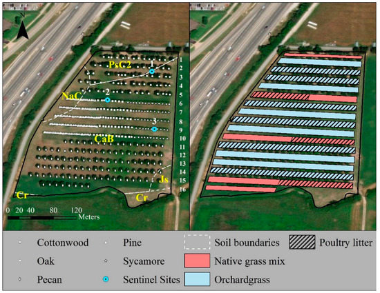
Figure 1.
Agroforestry site in Fayetteville, AR is organized into 16 rows, where Row 1 starts at the most-northern row. Rows 1–5 consist of the northern red oak; the western, central, and eastern portion of Rows 6–10 consist of the pitch/loblolly pine, cottonwood, and American Sycamore; and Rows 11–16 consist of pecan. The three sentinel site locations are located at a local summit (Sentinel Site 1), depression area (Sentinel Site 2), and mid-slope area between the summit and depression (Sentinel Site 3). The soils at the site include Captina silt loam (CaB), Pickwick silt loam (PsC2), Nixa cherty silt loam (NaC), Johnsburg silt loam (Js), and Cleora fine sandy loam (Cr; Soil Survey Staff, 2019b). The alleys between the tree rows consist of either orchardgrass or a native grass mix (big bluestem, little bluestem, and Indiangrass), where fertility treatments were fertilized with poultry litter in 2017- 2019. Maps were created in ArcGIS (ArcGISmap version 10.6.1, Esri, Redlands, CA, USA).
In 2000, sixteen rows of eastern black walnut (Juglans nigra L.), Northern red oak (Quercus rubra L.), and pecan (Carya illinoinensis Wangenh. K. Koch) were established and oriented east–west with 15 m of spacing between rows (Figure 1). The site was not ideal for growing eastern black walnut, where they grew adequately on the east end, but struggled to grow in the wet, middle portion and dry Nixa soil on the west end of the rows. As a result, the eastern black walnut trees were replaced in 2014 with rows that consisted of three different fast-growing species: American sycamore (Plantanus occidentalis L.) in the well-drained portion, cottonwood (Populus deltoides W. Bartram ex Marshall) in the poorly drained portion, and pitch/loblolly pine (Pinus rigida x Pinus taeda) in the drought-prone area of the field (Figure 1). Additionally, two forage-species treatments were established in the alleys between tree rows, including a cool-season species (orchardgrass (Dactylis glomerata L., var. Tekapo)) that was seeded in fall 2015 with 17 kg of pure live seed (PLS) ha−1 and a native warm-season mix (8:1:1 big bluestem (Andropogon gerardii Vitman), little bluestem (Schizachyrium scoparium (Michx. Nash) and indiangrass (Sorghastrum nutans L.) seeded in spring 2016 at 10 kg PLS ha−1 (Figure 1). A Haybuster 107C no-tillage drill (DuraTech, Jamestown, ND) was used to plant the alleys. Cornerstone® Plus (N-[phosphonomethyl] glycine, Winfield Solutions, St. Paul, MN, USA) was applied before establishment to rid the alleys of any existing vegetation at a 2.2 kg ha−1 rate (41% active ingredient (ai)), and alleys were treated with PlateauTM (ammonium salt of imazapic) after establishment at a 0.28 kg ha−1 rate (23.6% ai) to remove any remaining non-forage vegetation.
2.1.2. Fertilizer Applications
During every spring between 2001 and 2007, except for 2005, 3.9 to 6.7 Mg of poultry litter (PL) ha−1 was distributed via broadcast application over the eastern half of the AF site, and 50 to 76 kg nitrogen (N) ha−1—as the ammonium nitrate (NH4NO3) fertilizer—was broadcast-applied over the western half of the AF site [17]. In 2005, PL and NH4NO3 were applied at a rate of 8.9 Mg PL ha−1 and 123 kg N ha−1 in spring and fall, respectively [17]. Starting in June 2004, additional fertilizer was surface-applied to the surrounding ground near each tree as an annual application of Osmocote (The Scotts Miracle-Grow Co., Marysville, OH, USA), a slow-release fertilizer, that contained 5.6, 2.4, and 4.6 g of N, phosphorus (P), and potassium (K), respectively [17]. In 2005, both PL and NH4NO3 applications were made in the spring and fall to evaluate the impacts of nutrient source on soil physiochemical properties.
In March 2017 and 2018 and April 2019, orchardgrass and native grass treatments in the alleys between tree rows received 84 kg N ha−1 (4.94 Mg ha−1, fresh weight basis) of locally sourced PL (Figure 1). The chemical composition of the 2017 PL application was 2.7, 0.7, and 1.1% N, P, and K, respectively, and had a pH of 6.1. The 2018 PL had 2.0, 0.6, and 1.0% N, P, and K, respectively, and had a pH of 6.2. The 2019 PL had 2.5, 0.7, and 0.9 N, P, and K, respectively, and had a pH of 5.2. Additionally, the site was grazed by heifers (Bos taurus L.) at a density of 1.9 animal units (AU) ha−1 from May to June 2017, 2.2 AU ha−1 from May to July 2018, and 2.4 AU ha−1 from May to July 2019 [15,18,19]. Additionally, N, in the form of urea (46-0-0), was applied at a rate of 67.3 kg N ha−1 or 146 kg urea ha−1 on 30 March 2020 and 31 March 2021. Urea was applied to all alleys with a fertilizer spreader attached to a 3-point hookup with a spreading width of 15.2 m.
Between 2016 and 2021, the trees were annually individually fertilized in the spring/summer with variable rates and combinations of NH4NO3 or a 32-0-0 fertilizer (Oakley’s Carefully Blended 32-0-0 Fertilizer, Bruce Oakley, Inc., Little Rock, AR, USA), a 13-13-13 fertilizer (Greenkeeper’s Secret 13-13-13 Premium Fertilizer, T&M, Inc., Foristell, MO), and gypsum (CaSO4) The fertilizer combinations applied to the trees were based on fertility treatment and the tree fertilizer application rates were based on the nutrient concentrations of 2016 soil samples. Specific details on the 2016 to 2021 tree fertilizer amounts and application areas per tree species are presented on Table 1. Additional site establishment and management details have been reported [15,17,18,19,20,21,22,23,24,25,26,27,28,29,30].

Table 1.
Summary of the fertilizer types (i.e., NH4NO3, 13-13-13, gypsum (CaSO4)), amounts, and application areas of the fertilizers used to fertilize the trees (i.e., Northern red oak (Quercus rubra L.), pecan (Carya illinoinensis Wangenh. K. Koch), American sycamore (Plantanus occidentalis L.), cottonwood (Populus deltoides W. Bartram ex Marshall), and pitch/loblolly pine (Pinus rigida x Pinus taeda)) of an agroforestry site in Fayetteville, AR between 2016 to 2021.
2.2. Survey Equipment and Procedures
Geospatial, ECa measurements were obtained using a DUALEM-1S sensor (DUAL-geometry Electro-Magnetic; Dualem Inc., Milton, ON, Canada) and a Trimble R2 global positioning system (GPS) unit (Trimble Inc., Westminster, CO, USA; Figure 2). The DUALEM-1S operates at 9 kHz and has one transmitter, which uses a vertical dipole, and two receivers with different orientations [2,31]. The receiver has a 1 m separation from the transmitter and uses a vertical dipole in the horizontal coplanar geometry (HCP), which has a 1.1 m separation from the transmitter and uses a horizontal dipole in the perpendicular geometry (PRP) [2,31]. The depths of exploration (DOE) for HCP and PRP are ~1.6 and 0.5 m, respectively, where the DOE is defined as the depth to which an array accumulates 70% of its total sensitivity. Thus, HCP measures the bulk ECa of 0 to 1.6 m and the PRP measures the bulk ECa of the 0 to 0.5 m depth. The conductivity range for the DUALEM-1S is 3000 mS m−1 [2,31]. In this study, a Can-Am Side-by-Side (Defender, BRP US, Inc., Sturtevant, WI, USA) was used to power and pull the DUALEM-1S on a sled during surveying (Figure 2). Measurements from the DUALEM-1S were collected concurrently with the GPS data via a hand-held geoinformation system program (HGIS; HGIS version 10.90, StarPal Inc., Fort Collins, CO, USA) on a Trimble Yuma 2 rugged tablet computer (Trimble Inc., Westminster, CO, USA) [2,31].

Figure 2.
The apparent electrical conductivity (ECa) survey setup included a DUALEM-1S sensor (DUAL-geometry Electro-Magnetic; Dualem Inc., Milton, ON, Canada) that was suspended on a sled and tied to a Side-by-Side vehicle, and a Trimble R2 global positioning system unit (Trimble Inc., Westminster, CO, USA) mounted inside of the Side-by-Side; both the DUALEM-1S and Trimble R2 were connected to a Trimble Yuma 2 field computer inside the Side-by-Side that interpolated the data in a hand-held geoinformation system.
Monthly ECa surveys were conducted between August 2020 and July 2021 to capture the spatial and temporal ECa variability. To minimize the effects of temperature drift on the DUALEM-1S signal during surveying, surveys were conducted in the early morning and the DUALEM-1S sensor was powered on 30 min prior to each survey to allow the sensor to reach ambient temperature. For each survey, the DUALEM-1S was securely suspended on a sled, 12.7 cm above the sled bottom, and was pulled at a rate of 4.8 to 8.0 km hr−1 (Figure 2). The front of the DUALEM-1S was located 2.1 m behind the Side-by-Side and the center of the DUALEM-1S was located 4.15 m behind the Trimble R2 GPS unit (Figure 2). Each survey was conducted in a looping pattern over two alleys at a time until four parallel drive paths per alley, 2 to 5 m apart, had been achieved. During the survey period, unnecessary stops were avoided. After each survey, a calibration line was driven over all subsequent survey lines so that any drift that occurred in the DUALEM-1S’s measurement during the survey period could be monitored and accounted for. The calibration line was conducted in a “V” shape, starting in the northwest corner, ending in the southwest corner of the AF site, with the midpoint being around the eastern edge of Row 8 or 9 (Figure 1).
2.3. Weather and Soil Property Collection
Air temperature and precipitation was recorded every 30 min on a micrometeorological weather station, using a tipping bucket gauge, located 1.67 km away (36.10°N, 94.173°W) to the northeast of the northeast corner of the AF site. The recorded air temperature was averaged per day to obtain the daily average air temperature and the recorded daily precipitation was totaled to obtain the total daily precipitation. There were three sentinel sites at the study area and were located near the local summit, depression area, and a mid-slope area (Figure 1). In situ soil VWC and soil temperature were recorded every 4 h using 5TM soil moisture sensors (ECH2O 5TM Soil Moisture Sensor; METER Group, Pullman, WA, USA) at the 15 and 75 cm soil depths from the soil surface, and were logged on a Decagon EM50 data logger (METER Group, Pullman, WA, USA) at the sentinel sites (Figure 1). Additionally, ECa soil sensors were not able to be installed until 26 January 2021 at the study site; two EC sensors (Teros 12; METER Group, Pullman, WA, USA) were installed at the 15 and 50 cm depths at each of the three sentinel sites (Figure 1), where in situ soil ECa was measured every 4 h on a Decagon EM50 data logger. At the conclusion of the measurement period, VWC and soil temperature recorded between 1 August 2020 and 31 July 2021 and ECa recorded between 26 January 2021 and 31 July 2021 were averaged for each day and expressed as daily means.
During each survey, soil samples from 45 to 55 cm were collected at each sentinel site. Samples from the 0 to 15 cm soil depth were collected during each survey beginning on the 20 November 2020 ECa survey. Soil samples were placed in a plastic-lined bag and weighed in the laboratory. Afterward, samples were oven-dried in a forced-air oven at 70 °C for 48 h, re-weighed for moisture content, and then mechanically ground and sieved to <2 mm. Then, soil EC and pH were measured potentiometrically in a 2:1 water-volume-to-soil-mass slurry, where 40 g (±0.05 g) of the oven-dried, sieved soil was mixed with 40 mL of deionized water and reciprocally shook on a mechanical shaker for 1 h. The soil–water slurry was then filtered twice (No.1 filter paper, Cat No 1001 125; Whatman Cytiva, Little Chalfont, Buckinghamshire, UK) until there was 40 mL of filtrate; the filtrate was then mixed by pouring the filtrate back-and-forth between two plastic vails. Afterward, the volume of the filtrate was evenly split (20 mL) between the two plastic vials, and the pH and EC were determined by placing a pH (Orion 9107BNMD; Thermo Scientific, Waltham, MA, USA) and EC probe (Orion 013005MD; Thermo Scientific, Waltham, MA, USA) into each of the vials, whereby both were connected to a pH/Conductivity Benchtop Meter (Orion Star A215; Thermo Scientific, Waltham, MA, USA).
2.4. ECa Survey Data Processing
After collection, ECa survey data underwent data processing procedures, which included GPS coordinate adjustment, outlier removal, drift calibration, temperature adjustment, averaging of coincidental points, and universal-kriging. A spatial adjustment between the DUALEM-1S sensor and Trimble R2 GPS unit was performed to account for the 4.15 m difference between the location of the GPS unit and the sensor during data acquisition [32]. The ECa measurements were collected at an average speed of 6.4 km h−1 and the coordinates associated with each measurement were post-corrected to account for the distance between the center of the DUALEM-1S and the location of the GPS receiver. Furthermore, measurement points that had a PRP or HCP ECa measurement < 0.1 mS m−1 were removed from both the survey and calibration line, as ECa measurements < 0.01 mS m−1 were likely caused by the presence of metallic objects in the field. Additionally, measurement points that occurred within 2.0 m of soil sensor equipment at the AF site were removed to reduce the effect of magnetic interference in the ECa data [33,34]. Afterward, a Hampel filter [35] was applied to the PRP and HCP ECa data with a 10-point, half-width (i.e., 21-point moving data window) and a threshold of 3 using the pracma package [36] in R Studio (version 4.05, R Core Team, Boston, MA, USA) [37]. A Hampel filter normally replaces a determined outlier with the local median; however, in this case, any measurement point that was determined to be an outlier in the PRP and/or HCP ECa of the survey or calibration line was removed altogether to be consistent with earlier procedures.
Because internal temperatures of the DUALEM-1S increase during the survey period, ECa data can be slightly skewed and require calibration. To perform calibration, linear regression techniques were used to quantify the difference between the ECa of the survey points and the average ECa of the calibration points that occurred within 1.5 m of the survey points [32,34,37]. The projected differences between the ECa of the survey and the calibration line were subtracted from the ECa of the survey points at each time point, resulting in a drift-calibrated ECa survey dataset [32,34,37]. The calibration procedure was performed in R Studio using the geosphere package [38].
Because the ECa surveys were conducted throughout the year, the ECa of each survey occurred at a different soil temperature. As a result, it was necessary to standardize the ECa measurements to a reference temperature. The HCP and PRP ECa were both standardized to 25 °C (EC25) using the equation of Corwin and Lesch [5] (1):
where ECT (mS m−1) is the ECa at a particular soil temperature and T (°C) is the soil temperature [5]. The soil temperature used in Equation (1) was the average soil temperature of soil sensors at the three sentinel sites at the time of a particular ECa survey. Soil temperature measurements from a depth of 15 cm were used for the PRP ECa standardization, whereas measurements from 50 cm were used for HCP ECa standardization. Any measurement point that had an PRP and HCP ECa value of <0.1 mS m−1 after the EC temperature standardization Equation (1) was applied. Finally, the PRP and HCP ECa of any coincidental points were averaged, resulting in a final calibrated dataset.
After cleaning and processing, kriging methods were used to generate continuous raster layers from ECa point data. Twenty percent of the PRP and HCP ECa survey data were selected at random and set aside for model validation. The experimental semi-variogram was calculated with the remaining 80% and fitted with a nugget and exponential, spherical, Gaussian, Matern, circular, and linear models. The best model minimized the sum of square of error and was selected for universal kriging to a 5 × 5 m grid. Values from the interpolated raster were then extracted to each of the validation locations. The model residuals were calculated using Equation (2):
where is the residual value in location i, is the predicted value in location i, is the observed value in location i, and i belongs to all locations selected at random to form the validation dataset. The model error was calculated from model residuals using Equation (3):
where is the model error at location i. All interpolation procedures were conducted in R Studio using sp [39], rgdal [40], gstat [41], geodist [42], raster [43], and terra [44] packages.
2.5. Statistical Analyses
The cleaned, GPS-coordinate-adjusted, outlier-removed, drift-calibrated, temperature-adjusted, coincidental point-averaged, universally kriged PRP and HCP ECa survey datasets are hereafter referred to as PRP and HCP ECa. Multiple methods were used to accomplish Objective 1. First, the PRP and HCP ECa were used to determine the mean, SD, and CV among the 5 × 5 m pixels to assess the spatial variability of the AF site’s ECa during the 12-month study period. Furthermore, a one-factor analysis of variance (ANOVA) was conducted in R Studio to evaluate the effect of season and growing/non-growing season on PRP and HCP ECa. When main effect differences were found, the means were separated by least significant difference (LSD) at an alpha level of 0.05. The mean, SD, and CV of the PRP and HCP ECa per growing/non-growing season were determined by averaging the mean, SD, and CV for each survey that fell within the growing or non-growing season groups. The surveys that took place during the growing and non-growing season were determined using soil sensor and air temperature data recorded at or near the AF site along with guidelines provided by the NRCS’s National Water and Climate Center [45]. Table 2 summarizes each survey’s seasonal grouping (i.e., weather season and growing/non-growing season).
Table 2.
Summary of the seasonal (i.e., weather season (summer, fall, winter, and spring) and growing season (growing season and non-growing season)) groupings and the survey groupings compared against all 12 monthly conducted electromagnetic-induction (EMI) apparent electrical conductivity (ECa) surveys for the homogeneity of variance assessment. The EMI ECa surveys were conducted at an agroforestry site in Fayetteville, AR between August 2020 and July 2021.
To accomplish Objective 2, the k-means clustering algorithm [46] was used by overlaying and grouping PRP and HCP ECa surveys to generate the precision SMZs within the AF site. The optimal number of clusters used in the k-means clustering was determined using the factoextra package [47] in R Studio. Furthermore, Objective 3 was accomplished by conducting Pearson correlations among PRP and HCP ECa (independently and combined) and in situ, soil-sensor-collected VWC and ECa and benchtop-measured soil sample GWC, EC, and pH (at all depths) at an alpha level of 0.05. Additionally, to accomplish Objective 4, a Levene’s test for homogeneity of variance was conducted. The non-universally kriged PRP and HCP ECa survey datasets were used in the Levene’s test. There were five survey groupings of reduced quantity that were used to compare against the variability all 12 monthly surveys: surveys from the odd half of surveys in sequential order of conduction (H1), even half of surveys in sequential order of conduction (H2), middle of the season (MS), middle of fall and spring (MFS), middle of winter and summer (MWS). Table 2 also summarizes the survey groupings used in the Levene’s test.
3. Results
3.1. Weather, Soil Sensor, and Soil Sample Data
Temporal variations in soil properties followed temporal weather fluctuations throughout the sampling period of the study (i.e., 1 August 2020 to 31 July 2021). The AF site received a total of 818 mm of precipitation and the mean overall daily air temperatures at the AF site ranged from −18.7 to 28.3 °C. Additionally, the soil sensor daily mean soil temperature, VWC, and ECa ranged from 1.6 to 26.5 °C, from 9.9 to 57.7% (v v−1), and from 5.7 to 43.7 mS m−1, respectively (Figure 3). The soil sample GWC, EC, and pH ranged from 7.9 to 38.4% (m m−1), 6.3 to 27.9 mS m−1, and 4.6 to 6.7, respectively.
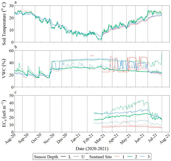
Figure 3.
The recorded daily mean soil temperature (temp; (a)), volumetric water content (VWC; (b)), and apparent electrical conductivity (ECa; (c)) for the upper (U; 15, 15, 15 cm, respectively) and lower (L; 75, 75, and 50 cm, respectively) soil sensor depths at Sentinel Site 1, 2, and 3, at the agroforestry site in Fayetteville, AR. Electromagnetic-induction ECa surveys dates are represented by the vertical dashed lines. Figures were created in R Studio (version 4.05, R Core Team, Boston, MA, USA).
3.2. ECa Survey Data
3.2.1. Monthly ECa Survey Data
The spatial pattern of the measured ECa was similar across all survey dates within both ECa configurations. For the PRP configuration, the September 2020 and June 2021 surveys had the lowest (0.2 mS m−1) and largest (29.1 mS m−1) recorded ECa values at the AF site during the sampling period, respectively (Table 3; Figure 4). The June 2021 survey had the greatest mean (8.7 mS m−1), SD (3.6 mS m−1), and range (26.4 mS m−1), and the September 2020 survey had the largest CV (48.1%) for the PRP ECa (Table 3; Figure 4). Furthermore, the September 2020 survey had the smallest mean (3.4 mS m−1), SD (1.7 mS m−1), and range (14.2 mS m−1), and the November 2020 survey had the smallest CV (32.2 %) for the PRP ECa (Table 3; Figure 4).
Table 3.
Summary of the perpendicular geometry (PRP) and horizontal coplanar geometry (HCP) apparent electrical conductivity (ECa) survey dates, number of measurements per survey, semi-variogram information (i.e., experimental model, nugget, sill, and range), and resulting summary statistics (i.e., mean, minimum (min), maximum (max), standard deviation (SD), and coefficient of variation (CV)) of each PRP and HCP ECa survey after universal kriging at an agroforestry site in Fayetteville, AR between August 2020 and July 2021.

Figure 4.
Spatial distribution of the universally kriged, perpendicular geometry (PRP) and horizontal coplanar geometry (HCP) apparent electrical conductivity (ECa) for the first (August-20), middle (January-21), and last (July-21) of the 12 monthly ECa surveys conducted between 2020 and 2021 at the agroforestry site in Fayetteville, AR. Maps were created in R Studio (version 4.05, R Core Team, Boston, MA, USA).
For the HCP configuration, the September 2020 and March 2021 surveys had the numerically smallest (0.4 mS m−1) and largest (34.2 mS m−1) recorded ECa values at AF site during the sampling period, respectively (Table 3; Figure 4). The December 2020 survey had the greatest mean (12.3 mS m−1), the June 2021 survey had the greatest SD (5.1 mS m−1), the September 2020 survey had the largest CV (61.1%), and the March and May 2021 surveys had the greatest range (29.4 mS m−1) for the HCP ECa (Table 3; Figure 4). Furthermore, the September 2020 survey had the smallest mean (6.7 mS m−1), the July 2021 survey had the smallest SD (3.9 mS m−1), the March 2021 survey had the smallest CV (35.5%), and the July 2021 survey had the smallest range (18.9 mS m−1) for the HCP ECa (Table 3; Figure 4).
3.2.2. Overall ECa Survey Data
The spatial patterns of the overall mean, SD, and CV differed greatly between PRP and HCP ECa. Averaged across all 12 surveys, the mean PRP and HCP ECa ranged from 1.8 to 18.0 mS m−1, and from 3.1 to 25.8 mS m−1, respectively (Figure 5), and shared a similar spatial pattern as the monthly surveys (Figure 4). The SD for PRP and HCP ECa ranged from 0.6 to 4.8 mS m−1 and from 1.3 to 4.9 mS m−1, respectively, across all surveys (Figure 5). Additionally, the CV for the PRP and HCP ECa ranged from 15.1 to 62.9% and from 7.3 to 54.6%, respectively, across all surveys (Figure 5). The PRP and HCP mean ECa, SD, and CV were unaffected (p > 0.05) by either the weather season or growing season.
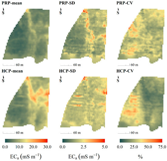
Figure 5.
The overall mean, standard deviation (SD), and coefficient of variation (CV) for all 12 universally kriged, perpendicular (PRP) and horizontal coplanar geometry (HCP) apparent electrical conductivity (ECa) surveys conducted between 2020 and 2021 at the agroforestry site in Fayetteville, AR. Maps were created in R Studio (version 4.05, R Core Team, Boston, MA, USA).
3.2.3. SMZ Delineation
Using the PRP and HCP ECa data, three precision SMZ were determined to be the optimal number of clusters at the AF site and were delineated using k-means clustering (Figure 6). The location and geospatial pattern of the SMZs were similar between the PRP and HCP (Figure 6) and both were visually similar to their respective overall means map (Figure 5). For both PRP and HCP ECa, SMZ 1, 3, and 2 (Figure 6) occurred where the recorded ECa was numerically smallest, in between, and the largest throughout the sampling period, respectively (Figure 5). With the exception of the CV, all summary statistics (i.e., mean, minimum, maximum, SD, and SE) for HCP were numerically greater than for PRP (Figure 6; Table 4). For both PRP and HCP, SMZ 2 was more variable (i.e., greater range, SD, and SE) than the other two SMZs (Figure 6; Table 4). However, when SMZs’ variability was standardized by the mean (i.e., CV), SMZ 1 had the numerically greatest variability relative to the mean compared to the other SMZs (Figure 6; Table 4). Additionally, SMZ 3 was generally the second numerically greatest occurring and second most variable (i.e., range, SD, CV, and SE; Figure 6; Table 4) among the three SMZs.
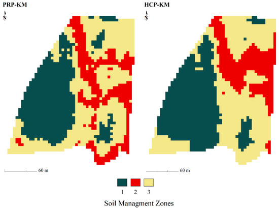
Figure 6.
Precision soil management zones (1–3) within the agroforestry site in Fayetteville, AR that were generated by the k-means (KM) clustering algorithm using all 12, perpendicular (PRP) and horizontal coplanar geometry (HCP) apparent electrical conductivity surveys. Maps were created in R Studio (version 4.05, R Core Team, Boston, MA, USA).
Table 4.
Summary of the perpendicular (PRP) and horizontal coplanar geometry (HCP) apparent electrical conductivity (ECa) for each cluster generated by the k-means clustering algorithm using 12 electromagnetic-induction ECa surveys conducted at an agroforestry site in Fayetteville AR between August 2020 and July 2021.
3.2.4. Correlations among ECa and Soil Properties
There were positive correlations between the ECa survey data (i.e., PRP, HCP, and combined (PRP and HCP)) and at least two measured soil properties (p < 0.05; Table 5). The HCP ECa and soil-sample GWC from the 45–55 cm depth interval (r = 0.71) and the PRP ECa and the soil-sample GWC in the 0–15 cm depth interval (r = 0.70) had strong, positive correlations (Table 5). The PRP ECa and the soil-sensor-measured ECa from the 15 cm soil depth (r = 0.84), the HCP ECa and the soil-sensor-measured ECa from the 50 cm soil depth (r = 0.74), and the combined ECa and the soil-sensor-measured ECa across soil depths (r = 0.65) also had strong, positive correlations (Table 5).
Table 5.
Summary of the resulting correlation coefficients (r) and p-values from Pearson linear correlations evaluating the relationship between the perpendicular (PRP), horizontal coplanar geometry (HCP), and combined (PRP and HCP) apparent electrical conductivity (ECa) and the upper, lower, and combined (upper and lower) soil-sensor-measured volumetric water content (VWC) and ECa measurements and the upper, lower, and combined soil-sample-derived gravimetric water content (GWC), electrical conductivity (EC), and pH, respectively. Electromagnetic-induction ECa survey, soil sensor, and soil sample data were collected from an agroforestry site in Fayetteville AR between August 2020 and July 2021.
The PRP ECa and the 15 cm, soil-sensor-measurement correlation was the only comparison where the soil-sensor-measured VWC was correlated to ECa survey data, but had a low correlation coefficient (r = 0.09; Table 5). Additionally, the HCP ECa and the 45–55 cm soil-sample-measurement correlation was the only comparison where the soil-sample-measured EC and pH were correlated to any ECa survey measurement. Specifically, HCP ECa and the 45–55 cm EC and pH had moderate, positive correlations (r = 0.37 and r = 0.42, respectively; Table 5).
3.2.5. Homogeneity of Variance Assessment
The homogeneity of variance was used to assess whether fewer, strategically selected ECa surveys could be conducted to capture the same amount of overall ECa variance at the AF site as the 12 monthly ECa surveys captured. The five reduced survey groupings that were used for the homogeneity of variance assessment are summarized in Table 2. For the PRP ECa, there were differences between the variance of all 12 surveys and the variance of all 5 of the reduced number of survey groupings (i.e., odd half of surveys in sequential order of conduction (H1), even half of surveys in sequential order of conduction (H2), middle of the season (MS), middle of fall and spring (MFS), middle of winter and summer (MWS); p < 0.05; Table 2 and Table 6). Except for when compared to the H1 survey group, the variance of all 12 PRP ECa surveys was greater than the variance of the other four reduced number of survey groupings (i.e., H2, MS, MFS, and MWS) for the PRP ECa (Table 6). In contrast to the PRP, for the HCP configuration, there were differences between the variance of all 12 monthly surveys and the variance of MS and MFS reduced groupings (Table 6). Specifically, the variance of all 12 monthly HCP ECa surveys was greater than the variance of both the MS and MFS groupings (Table 6). Conversely, there was no difference between the variance of all 12 monthly HCP ECa surveys and the reduced H1, H2, and MWS survey groupings (Table 6).
Table 6.
Summary of the homogeneity of variance between all 12 monthly perpendicular (PRP) and horizontal coplanar geometry (HCP) apparent electrical conductivity (ECa) surveys and five reduced survey groupings (i.e., H1, H2, MS, MFS, and MWS). Additional details of the survey groupings are presented in Table 2. Homogeneity of variance was evaluated using the Levene’s test.
4. Discussion
4.1. ECa Survey Data
4.1.1. Semi-Variogram Information
The semi-variogram range can be used to help understand the modeled variable (e.g., ECa in this study). The ranges of the PRP ECa surveys were 31 to 68% less than the ranges from the corresponding HCP ECa surveys (Table 3), which is indicative of the PRP ECa being more spatially erratic and variable than the HCP ECa [48,49]. DeCaires et al. [50] conducted repeated DUALEM-1S surveys on a 5.81 ha cacao (Theobroma cacao L.) plantation, classified as an alluvially formed silty-clay Inceptisol in Trinidad, and reported that the PRP ECa generally had a shorter range than the HCP ECa. The PRP ECa being more spatially variable than the HCP ECa is likely to be a result of the HCP measuring deeper into the soil profile than the PRP. Specifically, the PRP incorporates less of the soil profile into its measurement, and the part that is incorporated into PRP ECa measurement (i.e., 0–0.5 m) is generally much more variable in pedogenesis factors and soil properties (i.e., SWC, OM, nutrients, structure/porosity, and coarse fragments). The variations in pedogenesis and soil properties are the result of the upper portion of the soil being more exposed to surface factors that are also spatially and temporally variable, such as weather (i.e., precipitation, air temperature, wind, and sunlight), environmental processes (i.e., runoff, surface erosion/accumulation, and evapotranspiration), and land management (i.e., fertilizer/manure and type and quantity of trees/grasses/animals).
4.1.2. Monthly ECa Survey Data
Because PRP and HCP measure the bulk ECa of the 0–0.5 and 0–1.6 m soil depths, respectively, the measured PRP ECa was more likely to be a reflection of soil surface management, and the HCP ECa was more likely to be a reflection of pedogenic factors (i.e., time, parent material, organisms, topography/relief, and climate). Additionally, because different soils have varying properties, it can be expected that different mapped soils would result in varying ECa measurements across the AF site. However, based on the generated PRP and HCP ECa maps (Figure 4), soil boundaries were not detailed enough to show visual correlations with the measured ECa values for either ECa configurations. Although the soil boundary data were not detailed enough for visual correlations with the ECa data, the western portion of the AF site was still generally characterized by a shallower depth to bedrock and an increase in chert coarse fragment abundance (Figure 1). Coarse fragments have been shown to be negatively corelated with ECa [51]. Thus, the increased chert coarse fragments could have resulted in the decreased PRP and HCP ECa values in the western portion of the AF site (Figure 4).
An additional potential residual effect is that PL was applied between 2001 to 2007 and can be observed through increased ECa values occurring in the eastern half of the AF site in both ECa configurations (Figure 4). Specifically, PL and NH4NO3 were annually applied based on the annual soil total-N concentrations to the eastern and western halves of the AF site between 2001 and 2007, respectively [17]. After the PL and NH4NO3 applications, Sauer et al. [17] reported numerically larger percent changes in nutrient concentrations in 9 of the 11 soil nutrients measured (i.e., N, P, K, magnesium (Mg), sulfur (S), sodium (Na), iron (Fe), zinc (Zn), and copper (Cu)) in the soils that received PL, than the soils that received NH4NO3. Thus, increased nutrient concentrations likely remain in the soils that received PL and may be contributing to increased PRP and HCP ECa measurements (Figure 4).
In addition to PRP ECa most likely reflecting surface management, the PRP ECa likely varied overtime more than the HCP ECa due to variations in soil properties from fluctuating weather (i.e., soil moisture). Specifically, the SD for HCP ECa was generally more consistent than SD for PRP ECa (Table 3). Additionally, the SD for the PRP ECa was generally larger in the summer months than in the fall, winter, and spring (Table 3), which was most likely a reflection of increased soil moisture [48,52]. During wetter periods (i.e., fall, winter, and spring), the spatial distribution of soil moisture is heavily influenced by topography, where topography strongly controls the lateral distribution of water which increases soil moisture variability, and thus, the variability of measured ECa [48,52].
Although no surveys for either the PRP or HCP ECa were exactly alike, each survey per configuration had a similar geospatial pattern to the other (Figure 4). For both the PRP or HCP ECa, an elevated trail in ECa values can been seen starting in the northwest corner, peaking in the center (Rows 5 to 7), and trailing off to the bottom-middle of the AF site (Figure 4). This apparent pattern can be attributed to landscape properties that affect water flow and runoff accumulation and factors that affect measured ECa. Specifically, the trail of elevated ECa values occurs in the local drainage way of the AF site, where the northwest corner has the greatest elevation and the local landscape depression is in the center of Rows 5 to 7 (Figure 1 and Figure 4) [21,27]. Additionally, the runon from the surrounding, up-slope landscapes enters through a culvert in the northwest corner of the AF site (Figure 1). Overtime, overland flow results in the accumulation of water and transported nutrients, OM, and sediment in channels or low-lying areas, all of which increase measured ECa [3]. Thus, the elevated PRP and HCP ECa values in the northwest corner of the AF site towards the center of Rows 5 to 7 were most likely to be the result of greater SWC and accumulated transported materials from the local landscape, but also from the up-slope runoff entering into the northwest corner from the surrounding landscape (Figure 4).
Although more visible in HCP ECa surveys, two trails of elevated ECa values starting at the middle-eastern edge and connect to elevated ECa in the depression area can be observed in both configurations (Figure 4) [15,27]. Unlike at the local depressional area (Sentinel Site 2), no visual signs of soil wetness were observed in these areas during the duration of the study. However, the lower soil sensor at Sentinel Site 3, which was located at the more southern of the two trails of elevated ECa values, recorded similar VWC measurements as the upper soil sensor measurement at Sentinel Site 2 throughout the winter during this study (Figure 3). Additionally, Smith et al. [53] conducted ground-penetrating radar surveys at the AF site and produced measurements that potentially show groundwater movement in the same areas with elevated ECa values. Thus, the trails of elevated ECa values starting at the middle-eastern edge of the AF site are most likely due to increased SWC from a shallow groundwater table (Figure 4).
4.1.3. Overall ECa Survey Data
The mean HCP ECa being numerically greater than the mean PRP ECa was most likely a reflection of how soil properties vary with depth. Specifically, most of the AF site is classified as a Captina silt loam (Figure 1), which is characterized by a large increase in clay content with depth [14]. Additionally, fine-textured soil generally has a greater water-holding capacity and CEC than coarse-textured soil, and SWC generally increases with depth. Thus, the mean HCP ECa being numerically greater than the mean PRP ECa was most likely due to the SWC and clay content increasing with depth [3,48]. Additionally, measured soil ECa is influenced both by stable and dynamic soil properties. Numerous soil properties (i.e., soil texture, clay content, OM content, and depth to bedrock) are temporally stable within short time spans (i.e., within a year). Thus, within humid regions, including the southern Ozark Highlands, temporal fluctuations in the measured soil ECa are generally reflective of variations in SWC and water movement [48].
For both the PRP and HCP ECa, the SD was generally elevated in the NW corner and across the middle-eastern edges of the AF (Figure 5), where both were most likely a result of fluctuating SWC. The NW corner is where the runon from the surrounding, up-slope landscape enters the AF site. Therefore, runoff-producing precipitation events would cause the NW corner to have varying SWC, hence, varying ECa, throughout the year. Additionally, the elevated ECa across the middle-eastern edges of the AF site are likely to be where subsurface water movement occurs [53], and thus, fluctuation in the SWC in these areas would cause fluctuation in the measured ECa throughout the year (Figure 5). However, one major difference in the SD between the PRP and the HCP was that the PRP had elevated SD values along the drainage way at the site and the HCP did not (Figure 5) [15,21]. Elevated SD for the PRP, and not the HCP, was also likely to be from fluctuating SWCs throughout the year (Figure 5). Specifically, the PRP measures the upper 0.5 m of the soil, which is going to be more affected throughout the year by changes in weather and surface conditions (i.e., precipitation, air temperature, wind, sunlight, and evapotranspiration) than the 0–1.6 m of the soil profile which the HCP measures.
The CV of the PRP and HCP ECa generally had similar spatial patterns, where there were increased CVs in the west/southwest portion and decreased CVs occurring in the eastern portion, which slightly increase when moving towards the northeast of the AF site (Figure 5). However, the CV of the PRP ECa had a less cohesive pattern and was visually more variable across the AF site than that of the HCP ECa CV (Figure 5). The CV of the PRP ECa was visually more variable than the CV of the HCP ECa, which was potentially due to two reasons (Figure 5). First, the PRP ECa is a reflection of a smaller, upper portion of the soil profile (i.e., 0–0.5 m). Secondly, the 0–0.5 m portion of soil is generally more spatially and temporally variable in soil properties (i.e., SWC, OM, nutrients, structure/porosity, and coarse fragments) than the 0–1.6 m depth from the 0–0.5 m portion of the soil being exposed to surface factors that are also spatially and temporally variable (i.e., weather, environmental processes, and land management; Figure 5). Furthermore, the smallest CVs in the HCP ECa were generally located in wetter areas at the AF site [21], likely due to the deeper SWC in the soil profile at these locations being consistently moist-to-saturated throughout the year (Figure 5). Additionally, unlike the SD, there were no elevated CVs in the northwest corner or along the middle-eastern edges of the AF site for both ECa configurations (Figure 5). Thus, the ECa variability (i.e., SD) in the northwest corner and along the middle-eastern edges was minimal when standardized with the mean for both ECa configurations (Figure 5).
Elevated HCP, ECa, SDs, and CVs occurred under the pine tree canopies (Figure 5). There are several possible explanations for this, including a decreased water-holding capacity from a decreased effective soil depth, and an increased coarse fragment concentration in the Nixa cherty silt portion of the site (Figure 1) [22]. Additionally, it is possible that the coniferous trees may be acidifying soils relative to deciduous species at the site, thus, resulting in greater ECa, as Burgess-Conforti et al. [54] reported that coniferous was more acidic than deciduous leaf litter in northwest Arkansas.
4.1.4. Seasonal Effects on ECa
As a result of the PRP and HCP mean ECa, SD, and CV being unaffected (p > 0.05) by either weather season or growing season, there was no difference between the mean or variation (SD and CV) among surveys that were conducted in different weather seasons or surveys that were recorded in the growing season versus the non-growing season. Thus, the hypothesis that there would be significant differences between the ECa mean, SD, and CV of surveys that were conducted in different weather seasons and in the growing/non-growing season at a 20-year AF system within the Ozark Highlands was rejected. Although SWC is a major contributor to the measured ECa, other soil properties greatly contribute to the measured ECa in non-saline soil and are temporally stable (i.e., soil texture, BD, and CEC) [5], potentially helping to buffer ECa fluctuations caused by SWC variability. Thus, these results highlight that the measured ECa at the AF site was more reflective of and influenced by temporally stable soil (i.e., soil texture, clay content, OM content, BD, CEC, and depth to bedrock), vegetative (i.e., coniferous versus deciduous trees), and terrain properties than temporally variable soil properties (i.e., SWC) within short time spans (i.e., <1 year). Similar results have been reported by Harvey and Morgan [55] who conducted ECa surveys in spring 2005, fall 2005, and spring 2006 across four different fields in north-central Texas that primarily consisted of the Miles (Typic Paleustalfs) and Abilene (Pachic Argiustolls) soil series, and had been intensively cultivated with cotton (Gossypium hirsutum L.) and wheat (Triticum aestivum L.). Although the effect of season on the mean ECa or SD was not formally evaluated, Harvey and Morgan [55] reported relatively similar mean ECa and SD values for seasonal surveys. Additionally, Harvey and Morgan [55] also reported visual similarities among the kriged maps for the three surveys.
4.1.5. SMZ Delineation
Although SMZ 2 had greater numeric variability in the SD, SE, and range, SMZ 1 had the numerically greatest variability relative to the mean (i.e., CV) for both the PRP and HCP ECa (Figure 6; Table 4). However, SMZ 1’s numerically largest CV was more likely a result of the PRP and HCP mean ECa being 42 to 60% and 46 to 66%, respectively, than the other two SMZs, rather than a soil property or terrain attribute causing variability in the measured ECa within SMZ 1 (Figure 6; Table 4). Except for the CV, SMZ 2 had the numerically greatest mean and variability (i.e., range, SD, and SE) in the PRP and HCP ECa, which was most likely due to the accumulation of ECa-contributing soil constituents (i.e., OM, nutrients/salinity, clay, and water) and the largest SWC fluctuations of the three SMZs, from SMZ 2 encompassing the local drainage way and areas of potential subsurface water movement (Figure 6) [21,27,56]. Furthermore, SMZ 1 had the numerically smallest mean and variability in three out of four variability statistics (i.e., range, SD, and SE) in the PRP and HCP ECa, and was most likely due to SMZ 1 encompassing the area of a shallower depth to bedrock and increased coarse fragment abundance, and SMZ 1 not being a zone of accumulation (Figure 6) [21,26]. Although no soil sensor or sample data were collected from this area, SMZ 1 likely had the smallest VWC among the three SMZs for several reasons. First, SMZ 1 is not an area of water accumulation, thus, soil constituents (i.e., sediment, OM, and nutrients) have been eroded and less water is able to infiltrate into the soil, resulting in decreased SWC and SWC variability than in SMZ 2. Secondly, increased coarse fragments increases soil BD, which, in turn, decreases porosity, soil water-holding capacity, CEC, and VWC [57], and thus, ECa.
Zhu et al. [48] and Brevik et al. [58] reported larger soil ECa responses to SWC fluctuations at wetter positions in the landscape than in drier locations, suggesting that soil ECa is less dependent on SWC in drier locations than in wetter locations. Zhu et al. [48] also reported that at drier landscape positions or during drier time periods, the influence of water flow paths and SWC were masked by other soil and terrain attributes. Thus, the ECa values that resulted in the delineation of SMZ 1 and 2 could have been primarily influenced by SWC in SMZ 2, and primarily influenced by soil and terrain properties in SMZ 1 (Figure 6). Additionally, because measured ECa reflects the complex interaction of soil properties, terrain attributes, and vegetation, and the effects of different soil properties and terrain attributes were potentially able to be observed in each SMZ, the hypothesis that the monthly ECa surveys at a 20-year-old AF system within the Ozark Highlands could be grouped into similar functional populations and delineated into zones for precision soil management was confirmed.
The ECa-derived SMZs were produced in order to delineate soils with similar properties for precision/site-specific soil management. Adhikari et al. [21] created four topographical functional units (TFUs) at the AF site from a principal component analysis and k-means clustering of 13 terrain attributes (i.e., flow accumulation, slope length factor, mid-slope position, multi-resolution ridge top flatness index, multi-resolution valley bottom flatness index, normalized height, slope percent, slope height, system for automated geoscientific analysis wetness index, valley depth, and altitude above channel network). However, the four-terrain attribute-derived TFUs of Adhikari et al. [21] did not show any major visual similarities with the three ECa-derived SMZs created in this study (Figure 6). Additionally, for the actual management of this 4.25 ha AF site, the grid size would likely need to be increased from the current 5 × 5 m grid to perhaps a 10 × 10 m grid in order to improve the manageability of the AF site and its SMZs. As the topsoil is the layer that agricultural production is most concerned with, the PRP ECa configuration would be most beneficial to use when creating SMZs for precision soil management.
4.1.6. Correlations among ECa and Soil Properties
As a result of correlations between measured soil sensor/sample properties and measured ECa (Table 5), the hypothesis that monthly ECa surveys were correlated with soil-sensor- and/or soil-sample-based soil properties at a 20-year-old AF system within the Ozark Highlands was supported for some, but not all, soil parameters. With the exception of the sensor-measured ECa, GWC had the strongest correlation with ECa survey data in the PRP, HCP, and combined ECa datasets (Table 5). Thus, of the measured soil properties, GWC most likely contributed to the greatest extent of the measured ECa variability for both the PRP and HCP configurations (Table 5). Additionally, PRP and HCP ECa correlations were likely due to different soil properties (i.e., pH and EC) contributing varying degrees to ECa variability for PRP and HCP (Table 5).
The resulting ECa and soil property correlations were similar to previous results. Abdu et al. [2], Martini et al. [34], and Zhu et al. [48] conducted repeated ECa surveys with SMC measurements at fixed locations across each of their fields. Abdu et al. [2] conducted their study in north-central Utah over a soil of the Millville soil series (Typic Haploxerolls), Martini et al. [34] conducted their study in central Germany over soils primarily consisting of Cambisols, Luvisols, and Gleyols [59], and Zhu et al. [48] conducted their study in central Pennsylvania on Hagerstown (Typic Hapludalfs), Opequon (Lithic Hapludalfs), Murrill (Typic Hapludults), Nolin (Dystric Fluventic Eutrudepts), and Melvin (Fluvaquentic Endoaquepts) series. Similar to the results of this study, Abdu et al. [2], Martini et al. [34], and Zhu et al. [48] reported positive relationships between ECa and SMC. Using a Spearman rank correlation, DeCaires et al. [50] also conducted repeated ECa surveys and random soil sample measurements on a 5.81 ha cacao plantation with silty-clay Inceptisol soil in Trinidad and reported a strong positive relationship between both the PRP and HCP ECa and soil EC. Additionally, DeCaires et al. [50] reported significant relationships between PRP and HCP ECa and soil pH, and a weak, but significant, positive correlation between the PRP and HCP ECa and GWC. Furthermore, Corwin et al. [60] conducted one ECa survey and collected multi-depth soil sample measurements at a site classified as Panoche silty clay (Thermic Xerorthents) located within the San Joaquin Valley in central California. Corwin et al. [60] collected ECa and soil sample measurements for mapping and correlating ECa and soil properties to cotton yield variations and reported positive relationships between ECa at 0–1.5 m and 0–1.5 m GWC, EC, and pH.
4.1.7. Homogeneity of Variance Assessment
Similar ECa variances between groupings of ECa surveys with different quantities of surveys have implications on the quantity of ECa surveys necessary to capture the total temporal ECa variance of a study site. The variance of all 12 surveys being greater than the variance of the H2, MS, MFS, and MWS survey groupings for the PRP ECa is indicative that ECa surveys conducted every month for one year captured more numerical ECa variability than conducting six, four, or two evenly temporally spaced ECa surveys within a year (Table 6). Additionally, it is not clear why the H1 grouping for the PRP ECa had greater ECa variance than all 12 surveys combined; however, perhaps the greater ECa variance in the H1 grouping was potentially due to the H1 grouping dataset having fewer observations than the 12-survey dataset (Table 6). Alternatively for the HCP ECa, the variance of all 12 monthly surveys was greater than the variance of both the MS and MFS groupings, which is an indication that only conducting four HCP ECa surveys in the middle of the weather seasons (i.e., summer, fall, winter, and spring) or two HCP ECa surveys in the middle of fall and spring at this AF site would potentially result in not capturing all of the ECa variability within one year (Table 6). However, there was no difference between the variance of all 12 monthly HCP ECa surveys and the reduced H1, H2, and MWS survey groupings, which is an indication that only conducting six evenly temporally spaced HCP ECa surveys within a one-year period, or one HCP ECa survey in the middle of winter and summer, would be necessary in order to obtain the same amount of numerical ECa variability as 12 monthly HCP ECa surveys (Table 6). As a result, the hypothesis that fewer ECa surveys could have been conducted in one year to capture the same amount of overall ECa variance as the 12 monthly ECa surveys was supported for the HCP ECa, but not for the PRP ECa.
5. Implications
These results provide support for the applicability and ability of ECa surveys to look at in-field variability across agricultural systems and ecosystems. A better understanding of the tools and methods (i.e., EMI equipment and ECa surveys) that can be used to accurately assess soil property variability in spatially complex systems, such as AF, can improve the management and adoption of these conservation practices in areas prone to conservation issues (i.e., Ozark Highlands). Furthermore, ECa measurements and/or ECa-derived SMZs can be used as a blueprint for where to collect future soil samples, referred to as ECa-directed soil sampling [5,6,56]. Because ECa-derived SMZs delineate areas of potential differing soil properties, ECa-directed soil sampling can reduce the degree of soil surface disturbance and the quantity of necessary soil samples, and thus, time, energy, and cost spent on soil sampling compared to traditional grid soil sampling schemes [3,4,6,61]. Additionally, collecting soil samples and soil property data from each SMZ allows for the characterization of the most spatially and temporally influential soil properties affecting the measured ECa within each SMZ.
Apparent EC measurements and ECa-derived SMZs can also be used to explain crop yield variability. Specifically, the ECa-directed soil sampling method may be used to help characterize soil properties that are causing crop [4,60], forage, and/or tree growth variations. Through establishing SMZs and identifying soil properties that are most affecting their crop yield, producers have the potential to spatially and temporally target fertilizer, pesticide, and irrigation. As a result, SMZ-targeted resource applications have the potential to increase resource-use efficiency, yield, and profits, while reducing excess resource applications, loss of applied nutrients and pesticides, unintended environmental damage (i.e., surface and groundwater degradation), labor, and producer costs [62]. Additionally, establishing ECa-derived SMZs with soil property data before the establishment of an agricultural system can allow the producer to not only decide what type of crops to use and where to plant them, but also what type of agricultural system to establish in order to have the most productive agricultural system based on the present soil and land properties.
The ability to conduct fewer ECa surveys would be beneficial for researchers, agricultural consultants, and producers. Specifically, multiple surveys are necessary to assess the spatiotemporal variability of ECa measurements or soil properties, requiring additional soil surface traffic and time and resources spent collecting measurements. Thus, the ability to capture the same amount of ECa variability with fewer surveys would be beneficial for researchers, agricultural consultants, and producers due to the reduced time and energy spent collecting and processing the data; in addition, it would reduce surface traffic, which could positively contribute to maintaining soil surface health.
6. Conclusions
Identifying in-field variability and suitable methods to delineate soil property variations in AF systems may lead to greater adoption and better management in areas prone to conservation issues (i.e., Ozark Highlands). Previously, ECa surveys have been minimally applied in AF systems; thus, there is little information regarding the spatiotemporal relationship between repeated ECa surveys and soil property variations in AF systems, let alone AF systems within regions with similar features or conservation issues to the Ozark Highlands. Results of this study did not support the hypothesis that there would be differences between the ECa mean, SD, and CV of surveys that were conducted during different weather and growing/non-growing seasons. These results demonstrated that repeated ECa surveys can be used to assess the spatiotemporal pixel variation of the measured ECa of a 20-year-old AF system within the Ozark Highlands.
Results of this study supported the hypothesis that monthly ECa surveys can be grouped into similar functional populations and can be made into zones for precision soil management. Results of this study partially supported the hypothesis that monthly ECa survey data are correlated with soil-sensor-based VWC and ECa and soil-sample-based EC, GWC, and pH. Results of this study also partially supported the hypothesis that fewer, strategically timed, and evenly spaced ECa surveys could be conducted to capture the same amount of overall ECa variance at the AF site as the 12 monthly ECa surveys conducted. It is recommended that monthly ECa surveys are necessary to capture the full ECa variance at the 0–0.5 m soil depth within a 1-year period. However, to capture the full ECa variance in the 0–1.6 m soil depth of AF site within a 1-year period, it is recommended to conduct either ECa surveys every other month or one ECa survey in the middle of winter and summer to limit soil surface disturbance and to save resources. This study presents novel ECa surveys for use in precision management in a long-term AF system.
Results of this study provided beneficial and valuable insights on the spatial and temporal variability of ECa over time. Results demonstrated that a variety of methods can be used to assess spatial and temporal changes in measured ECa, and that the effects of pedogenic and anthropogenic factors on measured ECa can be observed in an AF system. Results of this study also demonstrated that ECa survey data are correlated to multiple soil properties and are used to create precision SMZs in an AF system within the Ozark Highlands. Thus, results of this study provide further evidence of the potential versatility, applicability, and ability of ECa surveys to quickly and accurately delineate in-field variability in different landscapes with different land uses and management systems.
Author Contributions
S.Y. conducted the ECa surveys, data processing, data analyses, and prepared the manuscript. A.J.A. and P.R.O. were responsible for conception of the research, securing and allocating funds in support of this research. H.S. and A.M.P. provided support in the use of R and GIS programs and in data processing procedures and analyses. K.R.B., A.J.A. and P.R.O. provided essential support, guidance, and consultation at each stage of this research. K.R.B., A.J.A., P.R.O. and A.M.P. reviewed and edited the manuscript. All authors have read and agreed to the published version of the manuscript.
Funding
Funding was provided by Foundation for Food and Agriculture Research (Grant No. 0000000025).
Data Availability Statement
The data presented in this study are available on request from the author.
Acknowledgments
Authors are grateful to Taylor Adams with the USDA-ARS for laboratory and field assistance and Watson Dunn for coding assistance. The mention of trade names or commercial products in this publication is solely for the purpose of providing specific information and does not imply recommendation or endorsement by the US Department of Agriculture.
Conflicts of Interest
The authors declare no conflict of interest.
References
- Garcia-Tomillo, A.; Miras-Avalos, J.; Dafonte-Dafonte, J.; Paz-Gonzalez, A. Mapping Soil Texture Using Geostatistical Interpolation Combined with Electromagnetic Induction Measurements. Soil Sci. 2017, 182, 278–284. [Google Scholar] [CrossRef]
- Abdu, H.; Robinson, D.A.; Boettinger, J.; Jones, S.B. Electromagnetic Induction Mapping at Varied Soil Moisture Reveals Field-Scale Soil Textural Patterns and Gravel Lenses. Front. Agric. Sci. Eng. 2017, 4, 135–145. [Google Scholar]
- Corwin, D.L.; Scudiero, E. Field-Scale Apparent Soil Electrical Conductivity. In Methods of Soil Analysis; Logsdon, S., Ed.; Soil Science Society of America: Madison, WI, USA, 2017; Volume 1, pp. 1–29. [Google Scholar]
- Corwin, D.L.; Lesch, S.M. Characterizing Soil Spatial Variability with Apparent Soil Electrical Conductivity—Survey Protocols. Comput. Electron. Agric. 2005, 46, 103–133. [Google Scholar] [CrossRef]
- Corwin, D.L.; Lesch, S.M. Apparent Soil Electrical Conductivity Measurements in Agriculture. Comput. Electron. Agric. 2005, 46, 11–43. [Google Scholar] [CrossRef]
- Johnson, C.K.; Doran, J.W.; Duke, H.R.; Wienhold, B.J.; Eskridge, K.M.; Shanahan, J.F. Field-scale Electrical Conductivity Mapping for Delineating Soil Condition. Soil Sci. Soc. Am. J. 2001, 65, 1829–1837. [Google Scholar]
- Heil, K.; Schmidhalter, U. The Application of EM38: Determination of Soil Parameters, Selection of Soil Sampling Points and Use in Agriculture and Archaeology. Sensors 2017, 17, 2540. [Google Scholar] [CrossRef]
- Agroforestry Practices. Available online: https://www.fs.usda.gov/nac/practices/index.shtml (accessed on 29 June 2022).
- Dollinger, J.; Jose, S. Agroforestry for Soil Health. Agrofor. Syst. 2018, 92, 213–219. [Google Scholar]
- Jose, S. Agroforestry for Ecosystem Services and Environmental Benefits: An Overview. Agrofor. Syst. 2009, 76, 1–10. [Google Scholar] [CrossRef]
- Brye, K.R.; West, C.P. Grassland Management Effects on Soil Surface Properties in the Ozark Highlands. Soil Sci. 2005, 170, 63–73. [Google Scholar] [CrossRef]
- Natural Resources Conservation Service. Land Resource Regions and Major Land Resource Areas of the United States, the Caribbean, and the Pacific Basin. In USDA Handbook 296; Government Printing Office: Washington, DC, USA, 2006; pp. 373–375. [Google Scholar]
- Major Land Resource Areas. Available online: https://data.nal.usda.gov/dataset/major-land-resource-areas-mlra (accessed on 23 June 2022).
- Web Soil Survey. Available online: https://websoilsurvey.sc.egov.usda.gov/App/WebSoilSurvey.aspx (accessed on 23 June 2022).
- Ashworth, A.J.; Adams, T.C.; Kharel, T.; Philip, D.; Owens, P.R.; Sauer, T. Root Decomposition in Silvopastures Is Influenced by Grazing, Fertility, and Grass Species. Agrosyst. Geosci. Environ. 2021, 4, e20190. [Google Scholar] [CrossRef]
- Data Tools: 1981–2010 Normals. Fayetteville Experimental Station, AR USA. Available online: https://www.ncei.noaa.gov/access/us-climate-normals/#dataset=normals-monthly&timeframe=81 (accessed on 23 June 2022).
- Sauer, T.J.; Coblentz, W.K.; Thomas, A.L.; Brye, K.R.; Brauer, D.K.; Skinner, J.V.; Brahana, J.V.; DeFauw, S.L.; Hays, P.D.; Moffit, D.C.; et al. Nutrient Cycling in an Agroforestry Alley Cropping System Receiving Poultry Litter or Nitrogen Fertilizer. Nutr. Cycl. Agroecosyst. 2014, 101, 167–179. [Google Scholar] [CrossRef]
- Niyigena, V.; Ashworth, A.J.; Nieman, C.; Acharya, M.; Coffey, K.P.; Philipp, D.; Meadors, L.; Sauer, T.J. Factors Affecting Sugar Accumulation and Fluxes in Warm- and Cool-Season Forages Grown in a Silvopastoral System. Agronomy 2021, 11, 354. [Google Scholar] [CrossRef]
- Gurmessa, B.; Ashworth, A.J.; Yang, Y.; Adhikari, K.; Savin, M.; Owens, P.R.; Sauer, T.J.; Pedretti, E.F.; Cocco, S.; Corti, G. Soil Bacterial Diversity Based on Management and Topography in a Silvopastoral System. Appl. Soil Ecol. 2021, 163, 103918. [Google Scholar] [CrossRef]
- Adams, T.; Ashworth, A.J.; Sauer, T. Soil CO2 Evolution Is Driven by Forage Species, Soil Moisture, Grazing Pressure, Poultry Litter Fertilization, and Seasonality in Silvopastures. Agrosyst. Geosci. Environ. 2021, 4, e20179. [Google Scholar] [CrossRef]
- Adhikari, K.; Owens, P.R.; Ashworth, A.J.; Sauer, T.J.; Libohova, Z.; Miller, D.M. Topographic Controls on Soil Nutrient Variations in a Silvopasture System. Agrosyst. Geosci. Environ. 2018, 1, 1–15. [Google Scholar] [CrossRef]
- Amorim, H.C.S.; Ashworth, A.J.; Sauer, T.J.; Zinn, Y.L. Soil Organic Carbon and Fertility Based on Tree Species and Management in a 17-Year Agroforestry Site. Agronomy 2022, 12, 1–13. [Google Scholar]
- Ashworth, A.J.; Kharel, T.; Sauer, T.; Adams, T.C.; Philip, D.; Thomas, A.L.; Owens, P.R. Spatial Monitoring Technologies for Coupling the Soil Plant Water Animal Nexus. Sci. Rep. 2022, 12, 3508. [Google Scholar] [CrossRef]
- DeFauw, S.L.; Brye, K.R.; Sauer, T.J.; Hays, P. Hydraulic and Physiochemical Properties of a Hillslope Soil Assemblage in the Ozark Highlands. Soil Sci. 2014, 179, 107–117. [Google Scholar] [CrossRef]
- Dold, C.; Thomas, A.L.; Ashworth, A.J.; Philipp, D.; Brauer, D.K.; Sauer, T.J. Carbon Sequestration and Nitrogen Uptake in a Temperate Silvopasture System. Nutr. Cycl. Agroecosyst. 2019, 114, 85–98. [Google Scholar] [CrossRef]
- Jiang, Z.-D.; Owens, P.R.; Ashworth, A.J.; Ponce, B.F.; Thomas, A.L.; Sauer, T. Evaluating Tree Growth Factors into Species-Specific Functional Soil Maps for Improved Agroforestry System Efficiency. Agrofor. Syst. 2021, 96, 479–490. [Google Scholar] [CrossRef]
- Kharel, T.P.; Ashworth, A.J.; Owens, P.R.; Philipp, D.; Thomas, A.L.; Sauer, T. Teasing Apart Silvopasture System Components Using Machine Learning for Optimization. Soil Syst. 2021, 5, 41. [Google Scholar] [CrossRef]
- O’Brien, P.L.; Thomas, A.L.; Sauer, T.J.; Brauer, D.K. Foliar Nutrient Concentrations of Three Economically Important Tree Species in an Alley-cropping System. J. Plant Nutr. 2020, 43, 2557–2568. [Google Scholar] [CrossRef]
- Thomas, A.L.; Brauer, D.K.; Sauer, T.J.; Coggeshall, M.V.; Ellersieck, M.R. Cultivar Influences Early Rootstock and Scion Survival of Grafted Black Walnut. J. Am. Pomol. Soc. 2008, 62, 3–12. [Google Scholar]
- Ylagan, S.; Amorim, H.C.S.; Ashworth, A.J.; Sauer, T.; Wienhold, B.J.; Owens, P.R.; Zinn, Y.L.; Brye, K.R. Soil Quality Assessment of an Agroforestry System Following Long-Term Management in the Ozark Highlands. Agrosyst. Geosci. Environ. 2021, 4, e20194. [Google Scholar] [CrossRef]
- Abdu, H.; Robinson, D.; Jones, S. Comparing Bulk Soil Electrical Conductivity Determination Using the DUALEM-1S and EM38-DD Electromagnetic Induction Instruments. Soil Sci. Soc. Am. J. 2007, 71, 189–196. [Google Scholar] [CrossRef]
- Simpson, D.; Lehouck, A.; Verdonck, L.; Vermeersch, H.; Meirvenne, M.; Bourgeois, J.; Thoen, E.; Docter, R. Comparison between Electromagnetic Induction and Fluxgate Gradiometer Measurements on the Buried Remains of a 17th Century Castle. J. Appl. Geophys. 2009, 68, 294–300. [Google Scholar] [CrossRef]
- Rudolph, S.; Wongleecharoen, C.; Lark, R.M.; Marchant, B.P.; Garré, S.; Herbst, M.; Vereecken, H.; Weihermüller, L. Soil Apparent Conductivity Measurements for Planning and Analysis of Agricultural Experiments: A Case Study from Western-Thailand. Geoderma 2016, 267, 220–229. [Google Scholar] [CrossRef]
- Martini, E.; Werban, U.; Zacharias, S.; Pohle, M.; Dietrich, P.; Wollschläger, U. Repeated Electromagnetic Induction Measurements for Mapping Soil Moisture at the Field Scale: Validation with Data from a Wireless Soil Moisture Monitoring Network. Hydrol. Earth Syst. Sci. 2017, 21, 495–513. [Google Scholar] [CrossRef]
- Pearson, R.K.; Neuvo, Y.; Astola, J.; Gabbouj, M. Generalized Hampel Filters. EURASIP J. Adv. Signal Process. 2016, 87, 1–18. [Google Scholar] [CrossRef]
- Borchers, H.W. Pracma: Practical Numerical Math Functions. R Package Version 2.3.3. 2021. Available online: https://rdrr.io/cran/pracma/ (accessed on 13 October 2022).
- Delefortrie, S.; Smedt, P.; Saey, T.; Vijver, E.; Meirvenne, M. An Efficient Calibration Procedure for Correction of Drift in EMI Survey Data. J. Appl. Geophys. 2014, 110, 115–125. [Google Scholar] [CrossRef]
- Hijmans, R.J. Geosphere: Spherical Trigonometry. R Package Version 1.5.10. 2019. Available online: https://rdrr.io/cran/geosphere/ (accessed on 13 October 2022).
- Pebesma, E.; Bivand, R.; Rowlingson, B.; Gomez-Rubio, V. Sp: Package Providing Classes and Methods for Spatial Data: Points, Lines, Polygons and Grids. R Package Version 2.0.7. 2005. Available online: https://rsbivand.github.io/sp/reference/00sp.html (accessed on 13 October 2022).
- Bivand, R.; Keitt, T.; Rowlingson, B. Rgdal: Bindings for the “Geospatial” Data Abstraction Library. R Package Version 1.5.23. 2021. Available online: https://www.rdocumentation.org/packages/rgdal/versions/1.5-32 (accessed on 13 October 2022).
- Pebesma, E.J. Gstat: Multivariable Geostatisitcs in S. R Package Version 2.0.8. 2004. Available online: https://www.rdocumentation.org/packages/gstat/versions/2.1-0 (accessed on 13 October 2022).
- Padgham, M.; Sumner, M.D. Geodist: Fast, Dependency-Free Geodesic Distance Calculations. R Package Version 0.0.7. 2021. Available online: https://hypertidy.github.io/geodist/ (accessed on 13 October 2022).
- Hijmans, R.J. Raster: Geographic Data Analysis and Modeling. R Package Version 3.4.10. 2021. Available online: https://rdrr.io/cran/raster/#:~:text=raster%3A%20Geographic%20Data%20Analysis%20and%20Modeling%20Reading%2C%20writing%2C,and%20for%20vector%20data%20operations%20such%20as%20intersections (accessed on 13 October 2022).
- Hijmans, R.J. Terra: Spatial Data Analysis. R Package Version 1.2.10. 2021. Available online: https://rdrr.io/cran/terra/ (accessed on 13 October 2022).
- Growing Season Dates and Length. Available online: https://www.nrcs.usda.gov/wps/portal/wcc/home/climateSupport/wetlandsClimateTables/growingSeasonDatesLength/ (accessed on 23 June 2022).
- Hartigan, J.A. Clustering Algorithms; John Wiley & Sons: Hoboken, NJ, USA, 1975; pp. 1–351. [Google Scholar]
- Kassambara, A.; Mundt, F. Factoextra: Extract and Visualize the Results of Multivariate Data Analyses. R Package Version 1.0.7. 2020. Available online: https://cran.r-project.org/web/packages/factoextra/readme/README.html (accessed on 13 October 2022).
- Zhu, Q.; Lin, H.; Doolittle, J. Repeated Electromagnetic Induction Surveys for Determining Subsurface Hydrologic Dynamics in an Agricultural Landscape. Soil Sci. Soc. Am. J. 2010, 74, 1750–1762. [Google Scholar] [CrossRef]
- Skøien, J.O.; Blöschl, G. Scale Effects in Estimating the Variogram and Implications for Soil Hydrology. Vadose Zone J. 2006, 5, 153–167. [Google Scholar] [CrossRef]
- DeCaires, S.A.; Wuddivira, M.N.; Bekele, I. Assessing the Temporal Stability of Spatial Patterns of Soil Apparent Electrical Conductivity Using Geophysical Methods. Int. Agrophys. 2014, 28, 423–433. [Google Scholar]
- Khakural, B.R.; Robert, P.C.; Hugins, D.R. Use of Non-contacting Electromagnetic Inductive Method for Estimating Soil Moisture Across a Landscape. Commun. Soil Sci. Plant Anal. 1998, 29, 2055–2065. [Google Scholar] [CrossRef]
- Western, A.W.; Blöschl, G.; Grayson, R.B. Geostatistical Characterization of Soil Moisture Patterns in the Tarrawarra Catchment. J. Hydrol. 1998, 205, 20–37. [Google Scholar] [CrossRef]
- Smith, H.; Ashworth, A.J.; Owens, P.R. Applications and Analytical Methods of Ground Penetrating Radar for Soil Characterization in a Silvopastoral System. J. Environ. Eng. Geophys. 2022. accepted. [Google Scholar]
- Burgess-Conforti, J.R.; Moore, P.A.; Owens, P.R.; Miller, D.M.; Ashworth, A.J.; Hays, P.D.; Evans-White, M.A.; Anderson, K.R. Are Soils beneath Coniferous Tree Stands More Acidic than Soils beneath Deciduous Tree Stands? Environ. Sci. Pollut. Res. 2019, 26, 14920–14929. [Google Scholar] [CrossRef]
- Harvey, O.R.; Morgan, C.L.S. Predicting Regional-Scale Soil Variability Using a Single Calibrated Apparent Soil Electrical Conductivity Model. Soil Sci. Soc. Am. J. 2009, 73, 164–169. [Google Scholar] [CrossRef]
- Corwin, D.L.; Scudiero, E. Mapping Soil Spatial Variability with Apparent Soil Electrical Conductivity (ECa) Directed Soil Sampling. Soil Sci. Soc. Am. J. 2019, 83, 3–4. [Google Scholar] [CrossRef]
- Chow, T.L.; Rees, H.W.; Monteith, J.O.; Toner, P.; Lavoie, J. Effects of Coarse Fragment Content on Soil Physical Properties, Soil Erosion and Potato Production. Can. J. Soil Sci. 2007, 87, 565–577. [Google Scholar] [CrossRef]
- Brevik, E.C.; Fenton, T.E.; Lazari, A. Soil Electrical Conductivity as a Function of Soil Water Content and Implications for Soil Mapping. Precis. Agric. 2006, 7, 393–404. [Google Scholar] [CrossRef]
- Food Agriculture Organization. FAO/Unesco Soil Map of the World, Revised Legend, with Corrections and Updates (Technical paper 20); FAO: Rome, Italy, 1988; pp. 1–146. [Google Scholar]
- Corwin, D.L.; Lesch, S.M.; Shouse, P.J.; Soppe, R.; Ayars, J.E. Identifying Soil Properties That Influence Cotton Yield Using Soil Sampling Directed by Apparent Soil Electrical Conductivity. Agron. J. 2003, 95, 352–364. [Google Scholar] [CrossRef]
- Johnson, C.K.; Mortensen, D.A.; Wienhold, B.J.; Shanahan, J.F.; Doran, J.W. Site-Specific Management Zones Based on Soil Electrical Conductivity in a Semiarid Cropping System. Agron. J. 2003, 95, 303–315. [Google Scholar] [CrossRef]
- Bongiovanni, R.; Lowenberg-Deboer, J. Precision Agriculture and Sustainability. Precis. Agric. 2004, 5, 359–387. [Google Scholar] [CrossRef]
Publisher’s Note: MDPI stays neutral with regard to jurisdictional claims in published maps and institutional affiliations. |
© 2022 by the authors. Licensee MDPI, Basel, Switzerland. This article is an open access article distributed under the terms and conditions of the Creative Commons Attribution (CC BY) license (https://creativecommons.org/licenses/by/4.0/).