1. Introduction
Since the onset of the Fast Track Land Reform (FTLRP) program in Zimbabwe and the subsequent redistribution and resizing of large-scale land holdings in the year 2000, plantation forests within and around the neighborhood of resettlement areas continuously faced physical distress [
1]. Zimbabwe lost close to 224,000 ha of tree cover, which is equivalent to a forest degradation of 17% and 88 Mt of CO
2 emissions from 2000 to 2021 [
2]. The steady decline of land under forest over the years has therefore been mainly driven by the activities of the year 2000 taking place on resettled land, which included wildfires, illegal logging, mining, and agriculture expansion. Yet the amount of additional biomass that can be accumulated in these areas depends much on the forest condition and land management practices.
A number of studies modeling the relationship between C stock and remote sensing-derived information adopt a standard approach where the effects of independent variables, including vegetation indices on C stock, remain constant over space in the model [
3,
4]. Given the history of Zimbabwe’s land reform program, it is well known that management and conservation practices of plantation forests have been changing over the years, particularly since the adoption of the program in the year 2000. Greater portions of formally designated commercial plantation forests were occupied and replaced by subsistence farmers across the country. It is upon this premise that it cannot be assumed that the impact of covariates on C stock is constant in these ecosystems. The carbon sequestration potential in various regions of the occupied forest plantations, therefore, remains unknown as the management and conservation practices of the managed ecosystems have been largely modified and altered [
5]. Yet government and other stakeholders in the timber industry are obliged under the 2015 Paris climate agreement to provide accurate accounts of the country’s carbon sequestration potential for managed and natural forest ecosystems.
The literature proffers methods used in the estimation of AGB, either as direct or indirect approaches from forest inventory data. These methods either use allometric equations, conversion factors such as wood density, or biomass expansion factors (BEF) [
1]. In spite of the advantages of using conventional methods given in [
6,
7] as generally providing accurate AGB estimates, these techniques are also regarded as time-consuming and environmentally unfriendly. The inaccessibility of some areas due to complicated topography and forest conditions also makes conventional methods less attractive to AGB estimation, especially in extensive areas [
8]. However, remote sensing is emerging as a promising technique free of the aforementioned limitations as it offers cost-effective methods of AGB monitoring through stratification of canopy density and forest types. Repeated application of remote sensing leads to the generation of historical data critical for change detection analysis and incorporation into a Geographic Information System (GIS) for integration with other datasets [
9]. However, remote sensing methods are also not immune from limitations as they usually face limitations in areas of bad weather conditions, especially in areas with cloud cover, and require a certain level of training for effective use and application [
7].
Remote sensing C stock data derived from satellite imagery has significantly grown over the years. This data has been the basis for informing international policy agreements associated with CO
2 emissions into the atmosphere, mainly from deforestation and other land use land cover changes (LULCC) [
10]. Remote sensing is regarded as a powerful tool for deriving AGB and forest structure as it offers practical means of acquiring spatially-distributed forest carbon from local, continental, and global scales [
5,
11]. Forest biomass can generally be measured from three broad categories of remote sensing (RS) data, namely, passive optical remote sensing, radio detection and ranging, microwave (radar), and light detection and ranging (LiDAR) [
8,
10]. Passive optical spectral reflectance is responsive to vegetation structural attributes (tree density, leaf area index, and crown size), shadow, and texture [
8,
12]. Crown size, tree density, and leaf area index (LAI) are strongly correlated with AGB. Radar remote sensing measure geometrical and dielectric attributes of forests. LiDAR RS methods of biomass measurement characterise forest vertical structure and height. Remote sensing (RS) and ancillary technologies such as Geographical Information System (GIS) are practical and cost-time effective, allowing for imaging and research on extensive and inaccessible areas.
The estimation of plantation forest C stock, together with other structural parameters using new regeneration multispectral remote sensing data, is a relatively new ground in the climate change and carbon monitoring arena. Research in this field has demonstrated the potential for remote sensing data as tools for developing estimates of forest attributes, amongst them, being Above Ground Biomass (AGB), either as a standalone or coupled with other earth observation techniques [
11,
13]. Spatial regression models applied in mapping C or biomass using new-generation multispectral remote sensing data may fail to clearly make room for residual spatial dependence [
14,
15]. Modeling of natural resource variables without explicitly accommodating spatial variation can be justified if covariates can account for all the spatially structured dependence. Such assumptions do not hold in many practical applications involving georeferenced data.
Failure to account for spatial dependence in the modeling of regionalized variables can lead to inaccurate model parameters and incorrect predictions [
9]. Subsequently, disregarding spatial correlation in electing model choices can result in higher prediction uncertainty for inference of the outcome variable. In addition to the drawbacks highlighted in the foregoing, non-Bayesian spatial modeling can further lead to underestimation of uncertainty [
9,
16] as traditional spatial regression estimation methods assume stationarity of the covariance matrix,
. The ultimate effect is the derivation of standard error estimates that are unable to take all the uncertainties in the parameters into account. Checking for spatially correlated residuals when spatial data are employed in the modeling of above-ground biomass is therefore critical.
Some attention has been given to spatially varying coefficient (SVC) models in the literature [
17,
18,
19]. The Bayesian framework of statistical inference is the bedrock of SVC models in which analyses make use of samples derived from Markov Chain Monte Carlo (MCMC) techniques from the posterior distribution of model parameters [
20]. What makes Spatially Varying Intercept (SVI) and SVC models unique in applied geostatistical and the remote sensing literature is their ability to consider the residual spatial dependence and the non-homogeneity in model parameters differently than ordinary geostatistical approaches. SVI models assume the model intercept is spatially varying, whilst the SVC models assume all the model regression coefficients to be spatially varying [
21]. A number of applications and methodologies utilizing spatially varying coefficient models are documented in the literature. Amongst them are the geographically-weighted regression (GWR) by [
21], who employed the technique of canopy height prediction using remote sensing data. Application of these models resulted in significant improvement in model fit. On the other hand, [
22] made provisions for spatial dependence and parameter non-homogeneity by exploring geostatistical kriging variants for forest canopy height prediction. Co-kriging and regression kriging models resulted in significant improvements in model fit.
However, it has been shown in recent times that GWR might not be robust to correlation among predictors and can potentially lead to inaccurate results when complex correlation structures are involved [
18,
23]. Again, from an inferential viewpoint, GWR can present problems when drawing inferences regarding prediction uncertainty and model parameters. The lack of valid underlying probability models in GWR makes prediction uncertainty, and standard parameter error estimates difficult to justify. For instance, uncertainty maps produced from kriging and co-kriging techniques make no consideration of the uncertainty in the variogram-based spatial covariance parameters. This is an established and common weakness encountered when using these geostatistical approaches [
24]. It is possible to estimate spatial covariance parameters within the SVC and SVI models using a Bayesian hierarchical construction. Such an approach allows the propagation of uncertainty to the prediction of the response variable [
25]. In such scenarios, a better and statistically defendable map of uncertainty can be produced than would else be produced when GWR or traditional kriging methods are utilized.
Landsat-8 and Sentinel-2 are multispectral platforms categorized as new generation remote sensing sensors with enhanced spectral and spatial properties than previous missions of the Landsat series. It is this perceived improvement in earth observation properties that we expect to give a dividend to C stock predictive models for applications in carbon accounting and inventorying under the United Nations Framework Convention on Climate Change (UNFCC) [
8]. We employed a Bayesian hierarchical framework with spatially varying coefficients (SVC) using predictor information derived from the aforementioned sensors for predicting C stock. The modeling framework considered the non-stationarity and residual spatial dependence of model covariates through the inclusion of spatial random effects into the SVC models. We, therefore, developed and compared the performance of C stock predictive models under spatially varying regression coefficients derived from Landsat-8 and Sentinel-2 predictors. Prediction accuracy and uncertainty quantification for the REDD collaborative program in the developing world is a critical aspect of the Carbon Measurement, Reporting, and Verification Systems (MRVs) of the United Nations (UN-REDD, 2009; CMS, 2014). Thus, in this paper, we explored how spatially varying coefficient models constructed using a Bayesian hierarchical set-up with aiding information from Landsat-8 and Sentinel-2 multispectral sensors and implemented through Markov Chain Monte Carlo (MCMC), perform in C stock prediction in plantation forest ecosystems.
2. Materials and Methods
2.1. Study Area
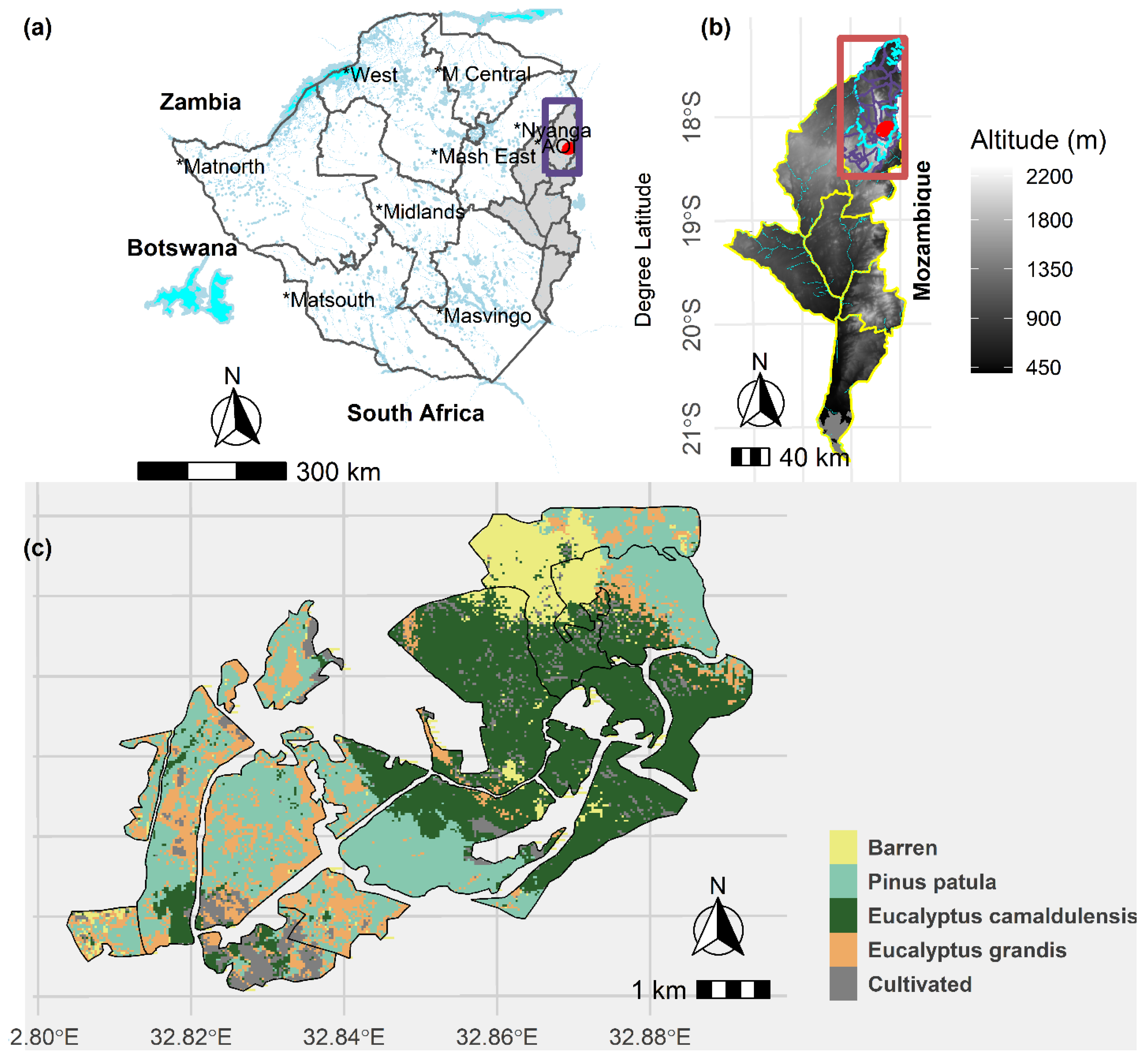
The study was carried out at lot 75 A of Nyanga Downs in Nyanga district in the Eastern Highlands of Zimbabwe (
Figure 1). The study area is dominated by
Eucalyptus grandis,
Eucalyptus camaldulensis, and
Pinus patula plantation forest species which have some of its patches being used for agriculture, grazing, and gold panning and is located between latitude 32°40′E and 32°54′E and 18°10′12″S and 18°25′4″S longitude as illustrated in
Figure 1 [
5,
26]. Grazing, agriculture, and gold panning activities came after part of the commercially owned plantation forests were redistributed to small and medium-sized indigenous farmers in 2000. This development has increased the interface between settlements and timber plantations in all forests originally designated under forest plantations in Zimbabwe. The study area covers an area of approximately 2766 ha. Rainfall amounts are varied, with a mean annual precipitation range of 741 mm to 2997 mm. Annual mean temperatures range from a minimum of 9 °C to 12 °C to a maximum of 25 °C to 28 °C. The weather is very hot, and extensive wildfires occur in the high-elevation grasslands from August to November when the grasses are dry [
26].
As illustrated in
Figure 1c,
Eucalyptus camaldulensis and
Pinus patula are the most dominant species in the study area. Pockets of cultivated land within the plantations are evident and are partly responsible for the present biomass density in the sampled region. Greater portions of former plantation vegetation have been cleared by pockets of resettled small-scale and medium-scale farmers venturing into coffee and tea plantations and, in some cases, for dairy farming. Patches of unprotected forest plantations are still present but remain vulnerable to attack for agriculture by settled farmers in the area.
2.2. Sampling Design
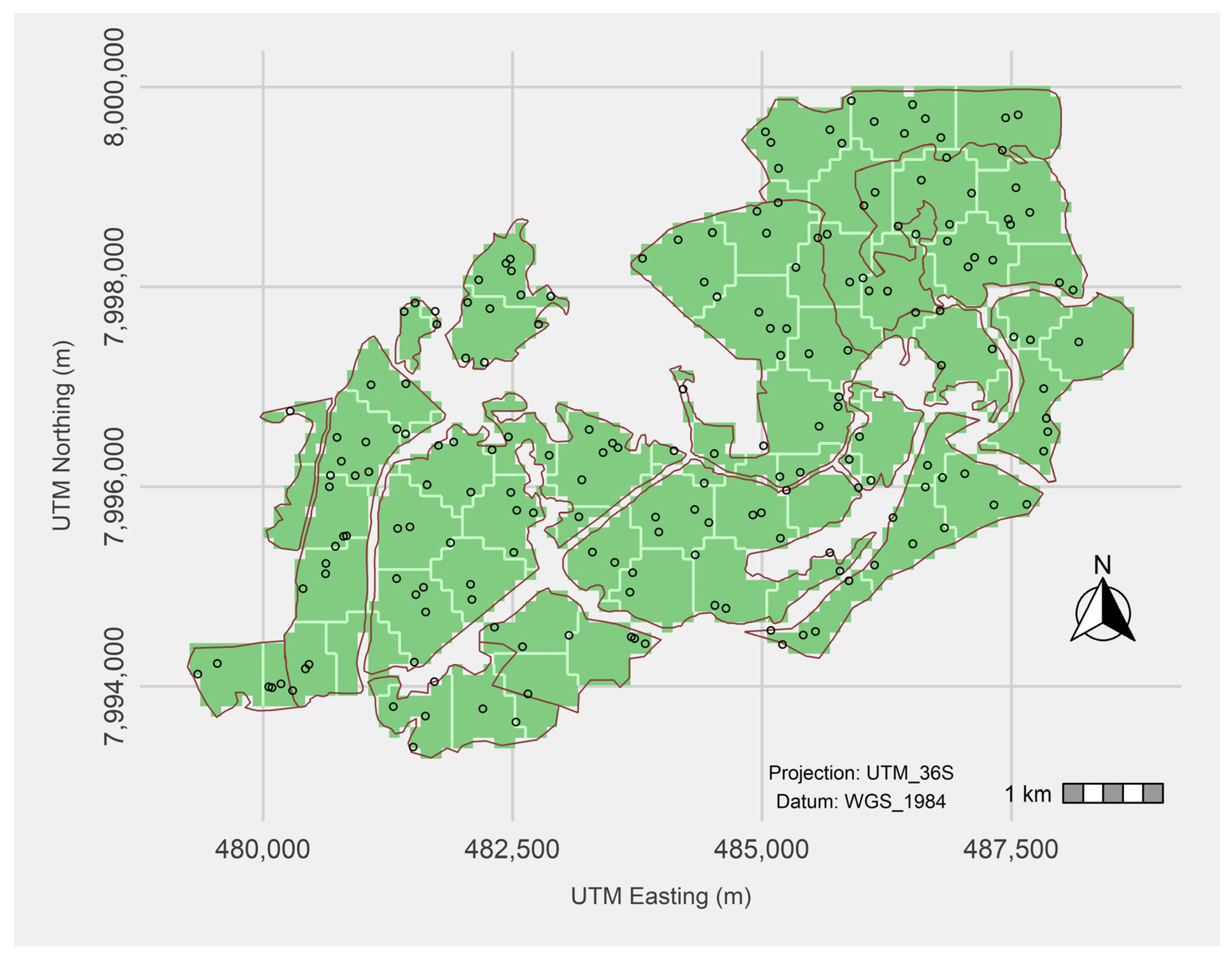
We employed the spatial coverage sampling scheme that exploits the Mean Squared Shortest Distance (MSSD) for the optimization of data locations in the study domain. The k-means clustering scheme for equal area coverage was therefore used [
27] for obtaining a representative sample from the studied region. The work of [
28] demonstrated how the mapping and estimation of mean spatial problems could be resolved through the employment of a uniform coverage sampling scheme. MSSD is particularly suited for areas where sampling campaigns cannot be extended beyond a single phase. As illustrated in
Figure 2, the smallest separation distance between samples was approximately 8 m whilst the largest separation distance between samples was 2500 m.
2.3. Above-Ground Biomass Measurements and C Stock Derivation
We sampled and collected measurements of Diameter at Breast Height (DBH) for Above Ground Biomass (AGB) estimation for all trees with a DBH of more than 10 cm (1.3 m) using 500 m
2 circular plots from the 19 September 2021 to 24 October 2021 in Manicaland Province of Zimbabwe as illustrated in
Figure 1. The sampling program meant to measure DBH for subsequent AGB and C stock estimation utilized the MSSD optimization function, resulting in 191 sampling plots being measured from the study area. The 191 sample plot measurements of DBH were then transformed into per plot C stock data using allometric equations of [
4] for the Pinus species, whilst the allometric equations of [
10] were used for deriving C stock for the Eucalyptus species. The aforementioned allometric equations were also applied by [
26].
Allometric equations shown in Equations (1) and (2) were used for the calculation of Above Ground Biomass (AGB) for the
Pinus patula and the Eucalyptus grandis and
Eucalyptus camaldulensis species, respectively [
1]. A default conversion factor of 0.47 used by the IPCC was applied to derive AGB to C stock.
2.4. Modelling Framework
It is a common geostatistical practice to assume at location
where
is a vector of observed
coordinates within the domain
. A Gaussian response variable
is therefore modeled through the regression model as in Equation (3):
denotes a set of covariates in the model. In this case, the linear mean structure accounting for wide-scale variation in the response is comprised of vectors of which include an intercept and spatially varying georeferenced predictors together with an associated column vector of model coefficients . The in the model represents a vector accommodating the intercept and those predictors from whose impact on the response is assumed to vary spatially. The space-varying impact is obtained from the vector of spatial random effects . The specification of different combinations of and the associated leads to the formation of different sub-models. We model as an independent white noise process that takes care of the micro-scale (measurement error) variation. As such, with the collection of C stock locations, , we assume the ’s are independent and identically distributed () as provided by where is the nugget.
The spatial structure of this model is generally introduced by way of a multivariate Gaussian process (GP) [
24,
25,
29] in which a cross-covariance function clearly models the covariance of
within and among data points. The added flexibility in this model is documented in the literature [
17,
30]. We assume in this study that elements of
emanate from
independent univariate GPs. Precisely, the process associated with the
prediction is
where
is a valid spatial covariance function modelling the covariance related to a pair of observations
and
. The process outcomes are gathered into an
vector, say
which permits a multivariate normal distribution
, in which
is an
covariance matrix of
with the
element provided by
. Evidently,
cannot just be a function, but guarantees that the resulting
matrix is positive definite and symmetric. Functions of this type are regarded as positive definite and are referred to as the characteristic function of a symmetric stochastic variable [
24,
25,
31].
We denote with to be a valid spatial correlation function in which computes the correlation decay rate and . We assumed for all the accompanying analyses an exponential correlation function , where represents the Euclidean distance between location and location . Completion of the Bayesian modeling framework requires specification and assignment of prior distributions to the parameters of the model, where inference proceeds by sampling from the posterior distribution of the modeled parameters. As standard practice, we assume prior where and , whilst the spatial variance components ’s and the measurement error variance are designated inverse-Gamma, priors. The spatial decay parameters with the lower and upper bounds of the distribution covering the geographic domain of the sampled study region.
Applying notation similar to the ones used by [
32], we can specify the model parameter posterior distribution as
where:
and is proportional to:
An effective Markov Chain Monte Carlo (MCMC) function for the estimation of Equation (4) is derived through updating of
from its full conditional and utilizing Metropolis procedures for the remainder of the parameters. Reparameterization of the model is an alternative way of ensuring the spatial random effects
do not require direct sampling [
33]. The spatial random effects could represent other independent variables that are spatially structured and not taken into consideration in the current modeling approach. Nonetheless, the MCMC process produces posterior samples of the parameter space,
.
From a prediction point of view, if
is a set of
new sites, the spatial random effects posterior predictive distribution corresponding to the
regression coefficient is provided by:
where
.
Since we are making use of MCMC sample-based inference, the integral in Equation (5) does not need to be evaluated precisely. Instead, given
posterior samples for the parameter space (
), that is,
, composition sampling can be used to derive this distribution [
33] by first drawing
followed by
for each
from
. The last distribution is multivariate normal as it is a derivative of a conditional distribution from a multivariate normal distribution. More specifically, the process realizations over the new sites are conditionally independent of the measured outcomes given the values over the sampled locations and the process parameters. Expressed differently,
is a multivariate distribution with mean and variance given by
and
where
is an
matrix with
element specified as
and
is an
n x n matrix with
element provided by
. Repetition of the same procedure results in the generation of samples for all the
’s. Lastly, for a set of predictors at unsampled locations
, posterior predictive distribution samples regarding the outcome variable
, are derived from
for
.
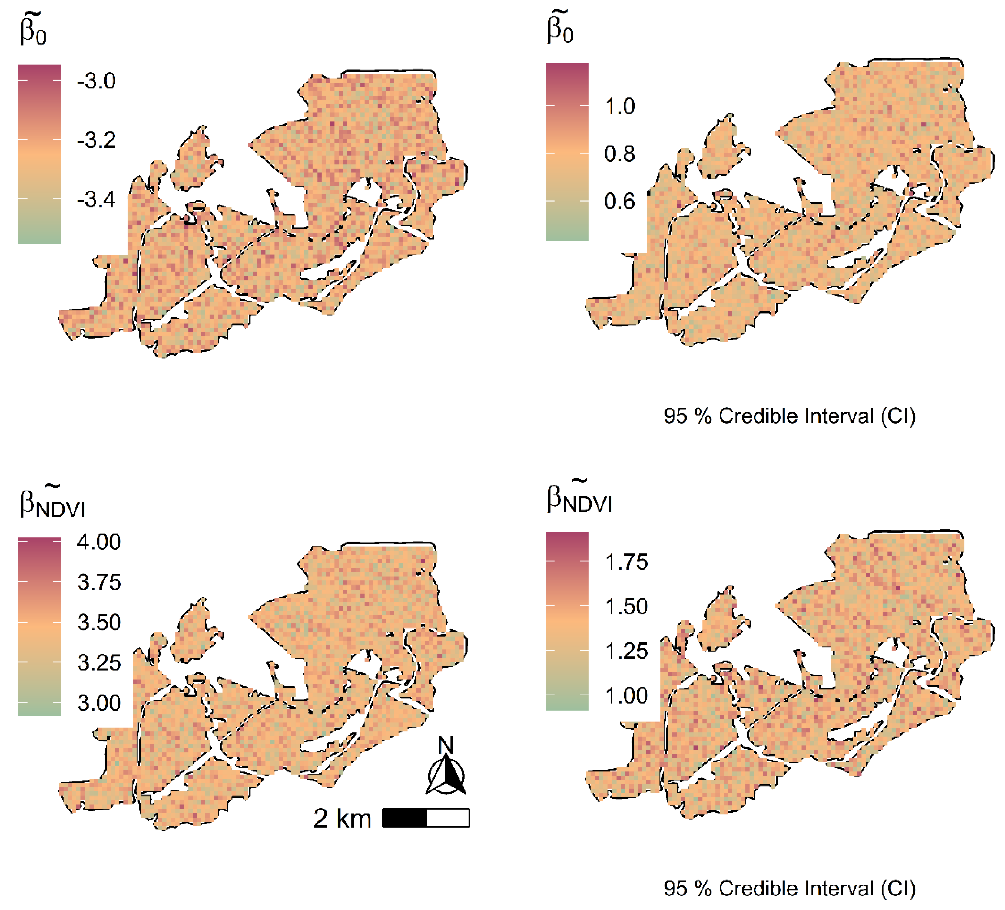
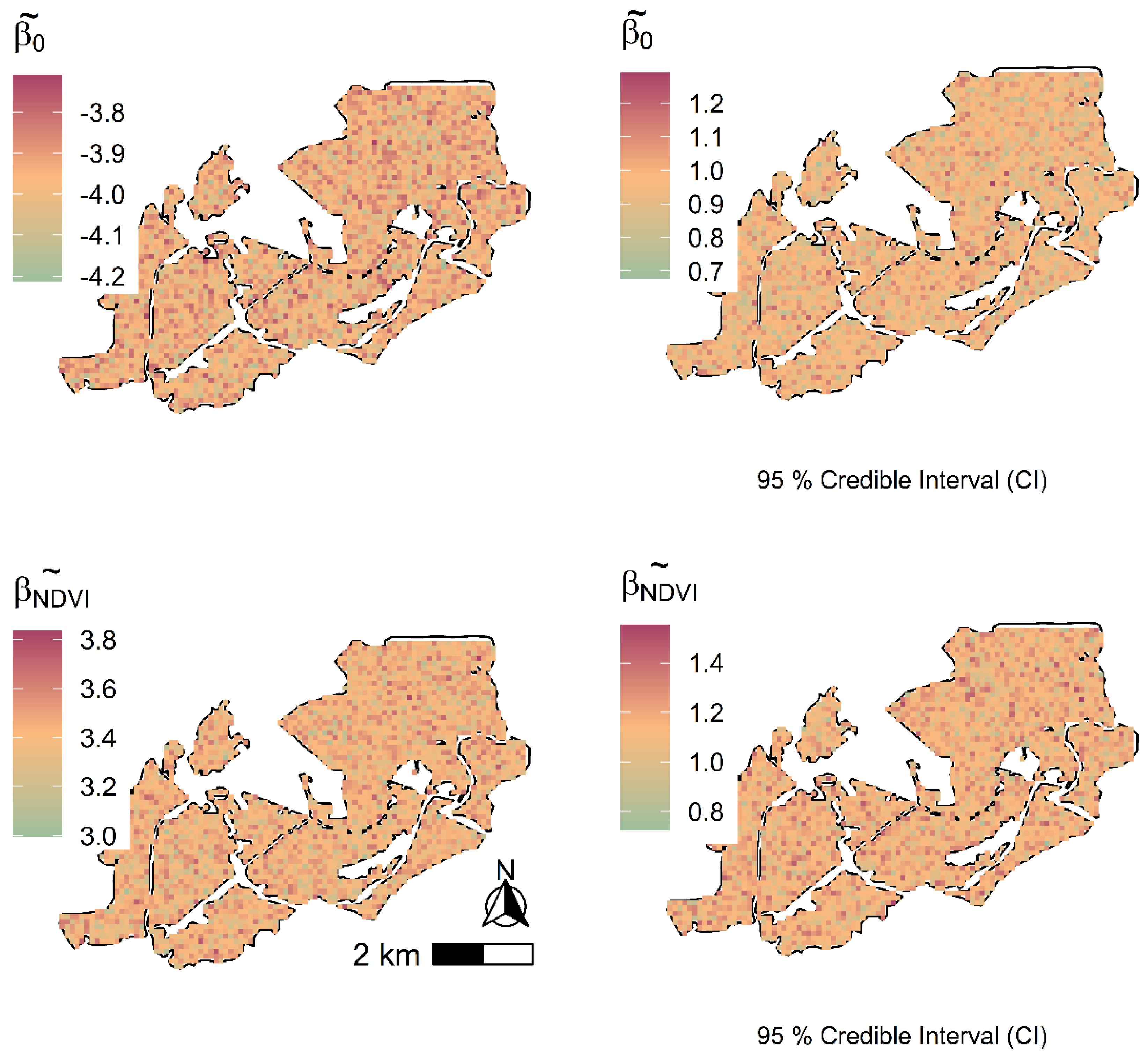
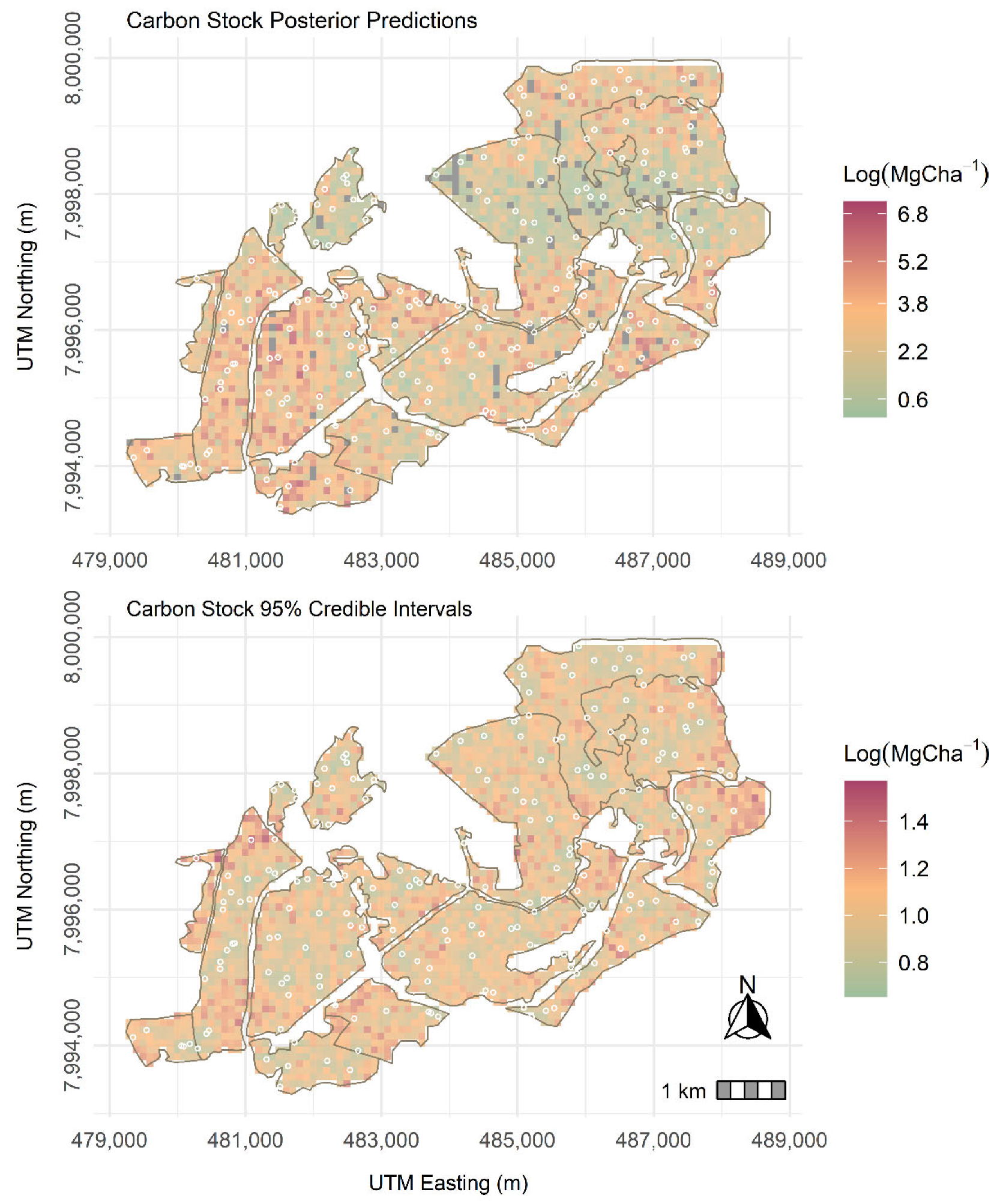
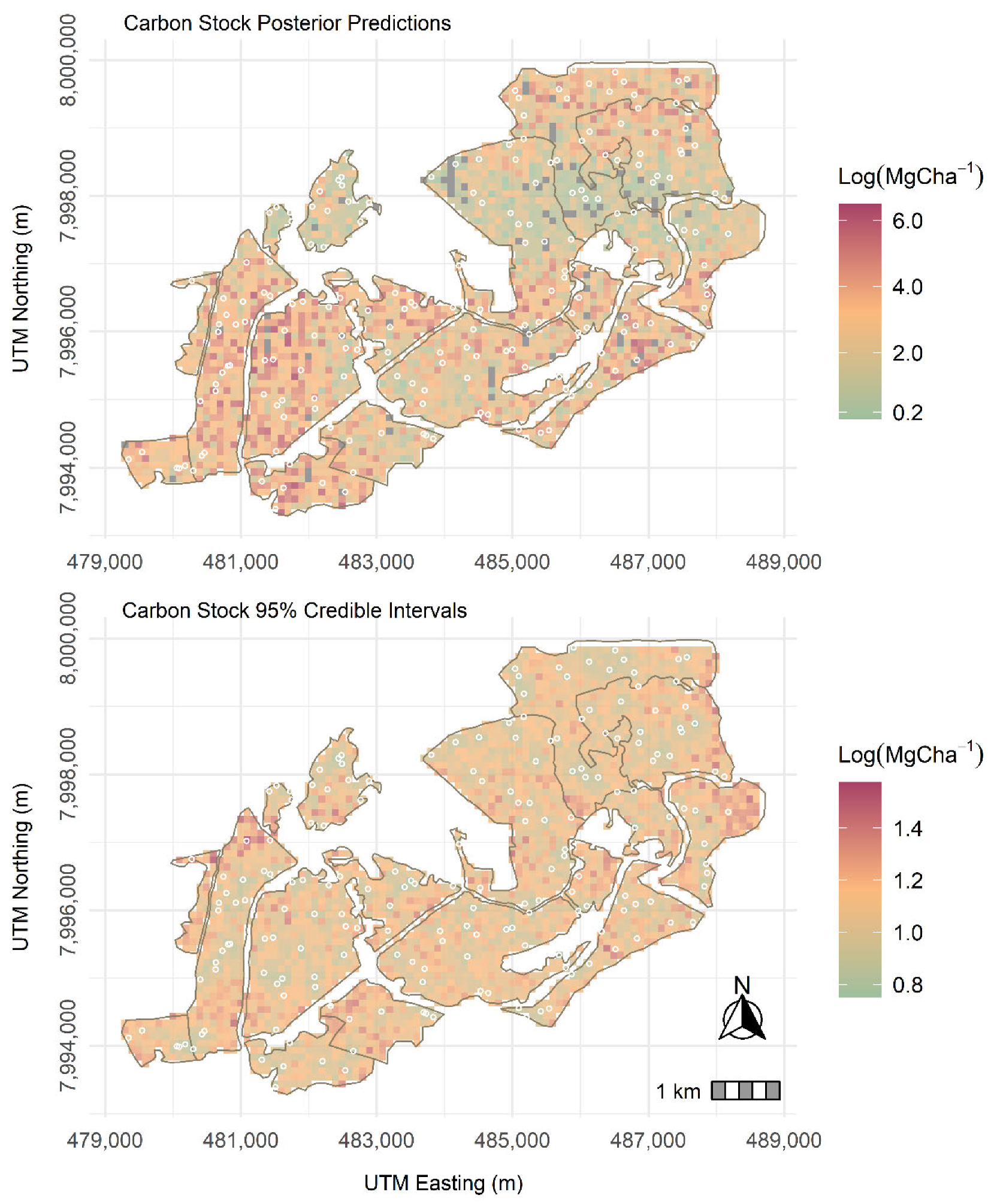
We evaluated 95% credible interval widths () using the posterior predictive distribution of Landsat-8 and Sentinel-2 C stock models by calculating the difference between the 2.5% and the 97.5% quantile bounds. The 95% were therefore used as summaries of the C stock prediction uncertainty for the Landsat-8 and Sentinel-2 C stock-based spatially varying coefficient models.
2.5. Competing Models
We derived five candidate models for each of the two multispectral remote sensing-based C stock models using Equation (1) using
and
as predictors of C stock [
34]. The models included the non-spatial where
’s is fixed to zero; the spatially varying intercept (
) in which we only included the spatial random effects related to the model intercept; the complete
model in which all predictors have associated spatial random effects; the
which included the spatial random effects for the intercept and
predictor variables and the
which included the spatial random effects for the intercept.
We utilized empirical semivariograms modeled for the residuals of the independent error model as guidelines for candidate model
and
hyperprior specifications. Precisely, for the variance parameters, the Inverse Gamma hyperprior
was set equal to
, which would result in a mean prior distribution equal to
and infinite variance [
35]. To add on, the models’
hyperpriors for the
and
’s were calibrated in accordance with the sample variograms of the simple linear regression model residuals derived from Landsat-8 and Sentinel-2 sensor’s nugget and partial sill. We programmed the prior for the spatial decay parameter
’s to
which, adopting the exponential covariance function, equates to support an effective range spanning between
and
. We define the effective spatial range as the distance where the correlation equals 0.05 [
18].
Three Markov Chain Monte Carlo (MCMC) chains were run for 20,000 iterations, each with the computationally demanding model requiring approximately 30 min to complete a single MCMC chain. We diagnosed convergence using the CODA library in the R Statistical and Computing environment by monitoring the mixing of chains and the Gelman–Rubin statistic [
36]. Acceptable convergence was established within 10,000 iterations for all the models. The posterior inference was premised on a post-burn-in subsample of 15,000 iterations, that is, every third sample from the last 15,000 iterations of each chain. SVC and SVI models were fit using the spBayes R Statistical and Computing Library version 0.4.3. We, therefore, utilized the spBayes R statistical package for fitting all the predictive models for both Landsat-8 and Sentinel-2 SVC models.
2.6. Landsat OLI and Sentinel-2 MSI Imagery Derived Covariates
Landsat-8 has a revisit period of 16 days and offers nine spectral bands with a spatial resolution of 30 m for Bands 1 to 7 and 9 [
6,
37]. The panchromatic band, Band 8, has a spatial resolution of 15 m. On the other hand, Sentinel-2 has thirteen spectral bands where four bands are configured at 10 m spatial resolution, six bands at 20 m, and three bands at 60 m spatial resolution [
37]. Common vegetation indices utilized in the estimation of biophysical variables of Absorbed photosynthetically active radiation (APAR), Leaf Area Index (LAI), and biomass are Normalised Difference Vegetation Index (NDVI), Enhanced Vegetation Index (EVI) and Soil Adjusted Vegetation Index (SAVI) [
5]. We utilized the same Vegetation Indices (VIs) in this study. Readily available and cost-effective new-generation sensors (Landsat-8 and Sentinel-2) with improved spectral and spatial resolution were therefore utilized in the modeling of C stock under the spatially varying coefficients assumption.
We obtained Landsat 8 imagery from the United States Geological Survey Earth Explorer (
http://earthexplorer.usgs.gov) as data ready for analysis (ARDs) on the 20 of September 2020. All the datasets were riddled with cloud cover and shadow cloud cover limits set to smaller than 10%. We acquired Sentinel-2 cloud-free images on 20 September 2020 at the same time as the Landsat 8 OLI data collection covering the entire area coinciding with the dates Landsat-8 OLI was collected covering the domain of interest. The multispectral instrument is the main imaging instrument used for Sentinel-2, a push broom scanner that measures the terrestrial Top of the Atmosphere (TOA) reflectance in thirteen spectral bands, that is, 443 nm to 2190 nm. We derived Sentinel-2 spectral data as level-1C 12-bit automated TOA reflectance values. Orthorectification and pre-processing of the TOA-derived products were performed using the sen2r package of the R Statistical and Computing environment [
38].
Soil Adjusted Vegetation Index (
), Enhanced Vegetation Index (
), and Normalized Difference Vegetation Index (
were used as Landsat-8 and Sentinel-2 derived covariates for C stock prediction in the plantation forest of the eastern highlands of Zimbabwe. The literature is replete with studies that have utilized the aforementioned vegetation indices [
3,
39] as ABG predictors in biomass estimation. In this study, predictor variables supplied by both Landsat-8 and Sentinel-2 are used specifically for comparing SVC Bayesian hierarchical geostatistical models predicting C stock in a disturbed environment in Zimbabwe. Given information regarding C stock distribution at each location, we fit the model in Equation (1)
with
. Hence, we have two processes, an intercept and one slope process relating to
.
2.7. Model Fit and Prediction Accuracy Evaluation
We assessed the performance of the models using the commonly used Deviance Information Criterion (DIC) to categorize models in terms of how well they fit the data [
40]. The sum of the Bayesian Deviance and the effective number of model parameters make up the DIC criterion. The Bayesian deviance measurement, which assesses model goodness of fit, and the effective number of model parameters which penalizes model complexity, are measured by D and pD, respectively. Attractive models have lower DIC values.
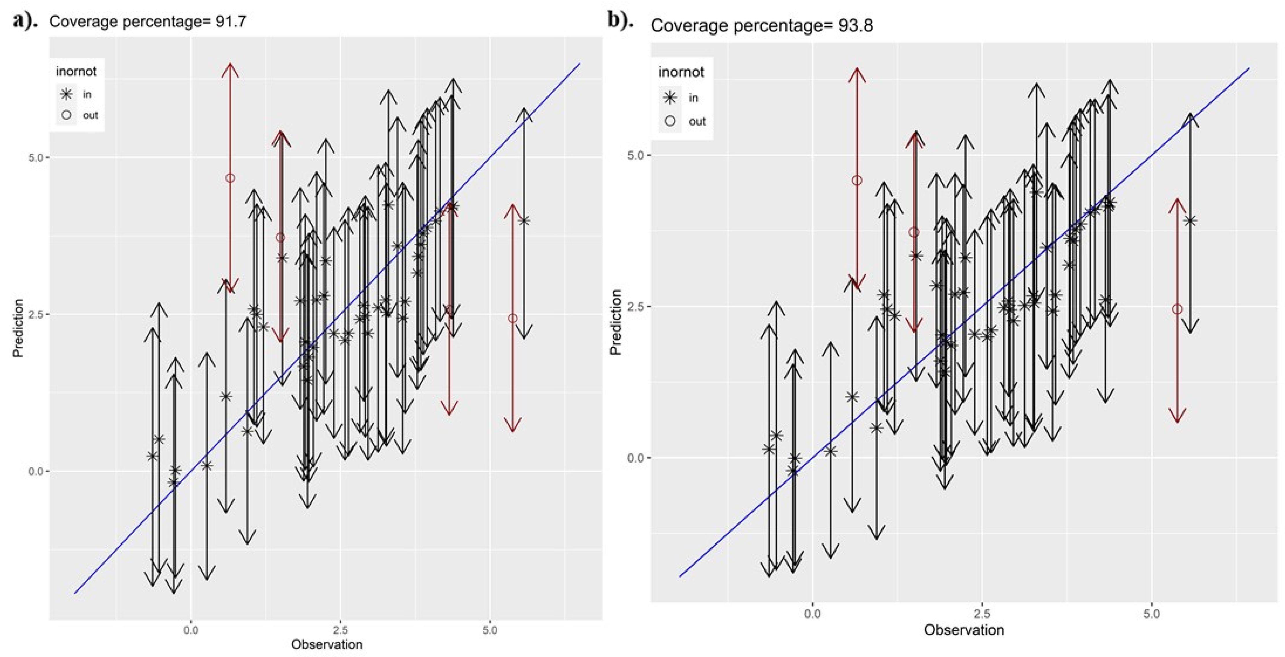
Predictive performance was evaluated through a cross-validation technique. C stock was predicted from observations within each subset, given the estimated parameters from the remaining subsets. We employed the Root Mean Squared Prediction Error (RMSPE) as a metric from the R Statistical and Computing environment to calculate the sampled C stock data values and the accompanying median of the posterior predictive distribution (PPD). Models with lower RMSPE signify more accurate C stock predictions.
4. Discussion
Space varying coefficient models constructed from different but related new-generation multispectral remote sensing platforms were used to predict C stock in a managed plantation forest ecosystem in Zimbabwe. The RMSPE is marginally higher in Sentinel-2-based C stock SVC model than in the Landsat-8-based SVC counterpart. Our findings with regard to the performance of Landsat-8 and Sentinel-2 sensors are also congruent with the work of [
12,
37]. SVC models for both new-generation remote sensing-derived predictors showed preference over the error-independent models. However, estimates from the two data sources were marginally different from each other on the prediction of C stock, as illustrated in validation diagnostics [
42]. The adaptable structure of the SVC permitted the residuals spatial variability to be apportioned between the random slope and the random intercept. This provided additional benefits not available in the SVI models from the two predictor sources. The SVC permitted reconnaissance of the C stock observations and the
predictor. Furthermore, the SVC models in both multispectral data sources had better representation of the processes thereby yielding C stock predictions with reduced variance.
Evaluation of the models utilizing predictors from both remote sensing data sources showed SVC to fit the data better than the SVI models. Kriged maps for C stock using Landsat-8 and Sentinel-2 data were not significantly different from each other, with the Landsat-8 SVC displaying a slightly wider 95% CI compared to the Sentinel-2-based SVC model. Again, this is partly because the study employed conventional bands (indices) that are calculated in a similar fashion in both Landsat-8 and Sentinel-2, and hence, the differences in prediction only emanated from the spatial resolutions. Explicit accommodation of residual spatial dependence through spatially correlated random effects gathered better predictions as the SVC models using the two data sources as regression coefficients borrowed additional information from neighboring C stock observations [
43,
44]. Precise estimates of covariance parameters are not easy to derive with small inventory sample sizes [
45]. Consequently, we might anticipate some impact on the accuracy of the predictions when uncertainty in the covariance ensues to the posterior predictive distributions. Predictions had limited information to borrow from because of the sparsity of C stock inventory observations. This was further worsened by the reduction in the overall sample size through cross-validation.
Similar to previous studies predicting ABG and C stock, our findings establish Sentinel-2 as a better source of RS data for predicting C stock in disturbed environments [
37] compared Sentinel-2 and Landsat-8 imagery for forest biomass prediction and showed Sentinel-2 outperforms Landsat-8 because of the enhanced spatial resolution in the former in comparison to Landsat-8. Most studies comparing Sentinel-2 and Landsat-8 for predicting AGB prefer Sentinel-2 over Landsat-8. This is further justified by the work of [
13], who compared Worldview-3, Sentinel-2, and Landsat-8 for representing AGB in a forest environment in Thailand and demonstrated Worldview-3 and Sentinel-2 as better data sources and, therefore, predictors than Landsat-8 due to the red-edge and the improved spatial and spectral properties of Worldview-3 and Sentinel-2. Furthermore, [
16] utilized LiDAR derived covariates from establishing the prediction performance of SVC models using forest inventory data in North America. The researchers established significant improvement in biomass prediction accuracy in the presence of residual spatial dependence deriving from the finer resolution LiDAR covariates. In most cases, the effectiveness of SVC models in these studies is usually strengthened by the solid non-stationary relationships between the response variable and the predictor variables influenced by unobserved ecological factors operating at broad geographical scales. Such ecological factors were also seen in the present study as NDVI was established to be a statistically significant predictors of C stock in the studied region. The biggest drivers to these factors are the presumed activities of forest disturbance due to human encroachment into plantation forests that subsequently impact the density and distribution of ABG biomass.
4.1. Limitations of the Study
Apart from the vegetation indices influencing the spatial distribution and density of AGB employed in this study, it is also known and acknowledged in the literature that climate and topographic variables play a part in the distribution of C stock. For example, [
37,
38] have shown elevation and aspect accounting for the bigger portion of the spatial variability of C stock in a mountainous region of Nepal. As such, the limitation of our study is the application of vegetation indices as predictors of C stock, and this may, therefore, not be representative of the general C stock dynamics in the studied region. We, therefore, recommend the integration of topo-climatic factors with new generation remote sensing-derived vegetation indices for future research in order to obtain a more accurate global overview of the C stock density and distribution in the studied region.
4.2. Conclusions
The study presented a hierarchical Bayesian geostatistical spatially varying coefficient model for determining the relationship between sampled C stock data and multispectral remote sensing derived predictors. There was a marginal improvement in model fit, and prediction accuracy in both Landsat-8 and Sentinel-2-based SVC models in comparison to the error-independent models. The SVC model permitted exploration of the observed C stock locations where the models performed well or poorly, which was missing in the SVI models. This provided an understanding of the performance of the multispectral remote sensing derived predictors for modeling C stock and hence, sets the foundation for the updating of the carbon forest plantation database for forest practitioners in the country and utilized as a monitoring tool in the long term. The Sentinel-2-based SVC model was preferred for prediction in the plantation forest ecosystems as its model provided tighter credible intervals compared to the Landsat-8-based C stock SVC model.
The small sample size of the data utilized in the present research enabled the modeling approach to be computationally feasible. When inventory plots are comprised of bigger sample sizes, the matrix operations of immense dimensions are needed for computing model parameter estimates of higher magnitude and may not be achievable through ordinary PCs. Our future work is therefore aimed at exploring algorithms for resolving the dimensionality curse when fitting spatially varying coefficient models. The problem of dimensionality can also get complicated if many predictors are involved in the SVC modeling framework. Resolving dimensionality issues is needed as forest C stock is typically modeled with predictors from many data sources, chief amongst them being topographic, bioclimatic, and anthropogenic variables.


