Communication

Global Terrestrial Water Storage Reconstruction Using Cyclostationary Empirical Orthogonal Functions (1979–2020)

by
Hrishikesh A. Chandanpurkar
1,2,3,*,
Benjamin D. Hamlington
1 and
John T. Reager
1
1
Jet Propulsion Laboratory, California Institute of Technology, Pasadena, CA 91109, USA
2
Global Institute for Water Security, University of Saskatchewan, Saskatoon, SK S7N 3H5, Canada
3
Centre for Sustainability, Environment, and Climate Change, FLAME University, Pune 412115, India
*
Author to whom correspondence should be addressed.
Remote Sens. 2022, 14(22), 5677; https://doi.org/10.3390/rs14225677
Submission received: 16 August 2022 / Revised: 26 September 2022 / Accepted: 2 October 2022 / Published: 10 November 2022
(This article belongs to the Special Issue Remote Sensing of Water Cycle: Recent Developments and New Insights)

Abstract

:
Terrestrial water storage (TWS) anomalies derived from the Gravity Recovery and Climate Experiment (GRACE) mission have been useful for several earth science applications, ranging from global earth system science studies to regional water management. However, the relatively short record of GRACE has limited its use in understanding the climate-driven interannual-to-decadal variability in TWS. Targeting these timescales, we used the novel method of cyclostationary empirical orthogonal functions (CSEOFs) and the common modes of variability of TWS with precipitation and temperature to reconstruct the TWS record of 1979–2020. Using the same common modes of variability, we also provide a realistic, time-varying uncertainty estimate of the reconstructed TWS. The interannual variability in the resulting TWS record is consistent in space and time, and links the global variations in TWS to the regional ones. In particular, we highlight improvements in the representation of ENSO variability when compared to other available TWS reconstructions.

1. Introduction

Terrestrial water storage (TWS), as observed by NASA’s Gravity Recovery and Climate Experiment (GRACE) [1] and GRACE Follow On (GRACE-FO) missions [2], represents vertically integrated water storage systems over global landmass (excluding ice sheets) and includes water stored in vegetation canopies, rivers and lakes (surface water), snow, soil (also called soil moisture), and groundwater. While little is known about the absolute amount of TWS, it is the spatio-temporal variability in TWS that directly relates to water availability (or a lack of thereof) for human and ecosystem use, and hence is of interest to a range of local-to-regional scale water resource researchers and managers. As TWS is a net residual of the terrestrial water balance between precipitation, evaporation, and runoff, its variability describes the changes in the overall water cycle. TWS change is also indicative of changes in the energy budget, since water and energy budgets are tightly coupled through changes in phase [3,4]. TWS, through soil moisture, is also closely linked with the carbon cycle [5]. Finally, changes in TWS directly correspond to the movement of water mass between land and ocean and are the dominant cause of interannual variability in global mean sea level (GMSL) (e.g., [6]).
While TWS has traditionally been a difficult state variable to measure globally, monthly global observations of TWS change have been made possible by the GRACE mission since 2002. GRACE can measure gravity anomalies for areas larger than about 200,000 km2, and at monthly to interannual time scales, these anomalies largely represent changes in water mass. GRACE ceased operations in mid-2017, and the GRACE-FO mission was launched in early 2018 to continue providing global TWS anomalies fields. GRACE data have been widely used in hydrology research from a regional to global scale on topics such as hydrologic extremes; human water management; analyzing changes in surface water, lakes and reservoirs, and groundwater; and better understanding of the natural and forced variability in storage at multiple timescales, including annual/seasonal variability, interannual variability—including that associated with the El Nino–Southern Oscillation (ENSO), and longer-term variability possibly associated with secular changes (see [1] for the wide range of GRACE application studies in earth sciences). However, compared to other terrestrial water cycle variables, such as precipitation, TWS data from GRACE still cover a relatively short period for attempts to robustly investigate interannual-to-decadal changes in terrestrial hydrology.
In recognition of the value of TWS observations and in an attempt to overcome the challenges presented by the relatively short satellite-measured record of TWS, increased focus has been put on extending the GRACE/GRACE-FO record back in time. A number of recent publications have tackled this topic using an array of approaches (e.g., [7,8,9,10,11,12,13]). The resultant reconstructions of TWS display a range of strengths and weaknesses, owing largely to the variability that is targeted or signal(s) of interest in each study. Providing direct comparisons between the datasets is then a challenge and can lead to conclusions assigned to a particular study that are outside of the original intent or objectives. Rather than introduce another technique to be evaluated broadly, we focused on establishing and implementing an approach that is targeted at interannual-to-decadal variability, and specifically the variability on those timescales that is driven by large-scale climate signals. Past studies have identified large shifts in global and regional TWS on these timescales and further connected these variations to ENSO (e.g., [6,14,15,16,17]).
In this study, we use a reconstruction technique based on cyclostationary empirical orthogonal functions (CSEOFs; [18]) to extend the GRACE record of TWS back to 1979. CSEOFs can be thought of as a special case of empirical orthogonal function (EOF) analysis where, unlike the standard EOF analysis, the eigenvectors (the spatial patterns commonly called EOFs) are not time-invariant and are allowed to vary within a specified period, commonly referred to as the “nested period.” This enables enhanced capturing of the quasi-periodicity of the natural climate variability modes within fewer modes than the traditional EOF analysis method. For example, in the standard EOF analysis, it is common to find that several modes together depict the annual cycle. In CSEOF analysis, these would get combined together as a single mode, allowing for a cleaner interpretation of the annual cycle. Kim et al., in 1996 [19], introduced CSEOFs specifically to capture the time-varying spatial patterns and longer-timescale fluctuations present in geophysical signals. Since then, CSEOFs have been used extensively to reconstruct historical regional and global sea-level variability based on relationships between tide gauges and satellite altimetry (e.g., [20,21]) as well as in multi-variate climate reconstructions [6,22]. The method has also been used to analyze spatio-temporal variability in TWS [16,23]. Recently, Hamlington et al. [6] applied the CSEOF method to reconstruct steric (ocean temperature) and barystatic (global TWS) components of the global mean sea-level budget and investigated the budget closure across a range of timescales (interannual to decadal).
Here, we extend and improve upon the CSEOF application in Hamlington et al. [6] to produce a reconstruction of TWS based on its common variability with precipitation and temperature. The improvements center on capturing regional-level variations while maintaining consistency with the global-level variations, ensuring orthogonality between the precipitation- and temperature-driven TWS patterns, and providing a time-varying estimate of uncertainty. The use of CSEOFs provides advantages by leveraging large-scale space-time patterns that serve as the basis for the reconstructed dataset. This yields estimates of interannual variability in TWS that are consistent in space and time and that link the global variations in TWS to those that occur on regional scales. In particular, we highlight improvements in the representation of ENSO variability in the resulting TWS record when compared to other available TWS reconstructions.

2. Data and Methods

2.1. Data

JPL GRACE/GRACE-FO Mascon Release 6 Version 2 (https://grace.jpl.nasa.gov/data/get-data/jpl_global_mascons/, accessed on 12 February 2021) was used for TWS training observations in this study. The data consist of monthly gravity field variations in terms of 4551 equal-area 3 spherical cap mascons [24,25]. While gain factors are included with the datasets which scale the intra-mascon variability of the mass changes, the gain factors were not applied in this study, since we were interested in the large-scale (beyond 3°) mass changes. We did use a version of the mascon dataset that includes a coastline resolution improvement (CRI) filter to separate land and ocean portions of water mass within each land/ocean mascon.
Terrestrial precipitation from Global Precipitation Climatology Project version 2.3 (GPCP, [26]) and 2 m temperature fields from the European Centre for Medium-Range Weather Forecasts (ECMWF) Reanalysis v5, commonly known as the ERA5 reanalysis [27], were used to identify relationships with GRACE TWS anomalies and for the reconstruction. While not pure observations, GPCP and ERA5 represent the widely used and most recent representations of the variables that are spatially and temporally consistent, have global coverage, and extend back considerably longer than GRACE. Hence, in this study they were used as proxies for observed precipitation and temperature. The backward extension of TWS anomalies is hence bounded by the start date of GPCP precipitation, 1/1979. While there are other precipitation products that have longer record lengths that also cover the pre-satellite era, we focus on the satellite era for consistency.
Additionally, the Multivariate ENSO Index (MEI) [28] was used for global-scale comparison and evaluation. TWS estimates from Global Land Data Assimilation System V2 (GLDAS V2, NOAH model) [29] and two other TWS reconstructions—one by Humphrey and Gudmundsson, 2019 [7] (hereafter referred to as HG2019), and the other by Li et al., 2021 [8] (hereafter referred to as Li2021)—were used for regional-scale comparisons.

2.2. Methods

Precipitation and temperature datasets were interpolated to the 0.5 × 0.5° resolution of the GRACE mascon solution using bilinear interpolation, and the global ocean and the two ice sheets were masked out. All data were trimmed to the overlapping GRACE duration and were normalized by their variance in order to be unitless. Below are the steps involved in the reconstruction algorithm.

2.2.1. TWS Reconstruction Algorithm

Step 1. Joint CSEOF decomposition was performed on GRACE TWS and GRACE-era precipitation (2002–2020) following Hamlington et al. [6] and using a nested period of 12 months to obtain dominant modes that are common between TWS and precipitation. A schematic showing the major steps involved in a typical CSEOF-based data extension can be found in Figure 1 in Hamlington et al. [6].
Step 2. Ten most dominant modes that explained about 95% of the variance in TWS and precipitation were identified.
Step 3. These modes were then extended using the entire duration of precipitation (1979–2020) to obtain a reconstruction of TWS (1979–2020), following [6].
Step 4. This reconstruction was then subtracted from GRACE observations to obtain a residual TWS for the GRACE-era.
Step 5. Steps 1–3 were repeated but with temperature instead of precipitation, and with residual TWS instead of GRACE TWS.
Step 6. The TWS reconstruction output from steps 3 and 5 were added together to create a final reconstruction of TWS.
The algorithm thus computed TWS reconstructions twice, once based on the common modes between TWS and precipitation alone (Steps 1–3), and once using the common modes between residual TWS and temperature (Step 5). Subtracting the precipitation-based TWS reconstruction from the observed TWS (Step 3) and using it as an input for temperature-based reconstruction ensured orthogonality between precipitation- and temperature-driven TWS patterns. In the following sections, the reconstructed TWS time series is referred to as TWS_CSEOF.

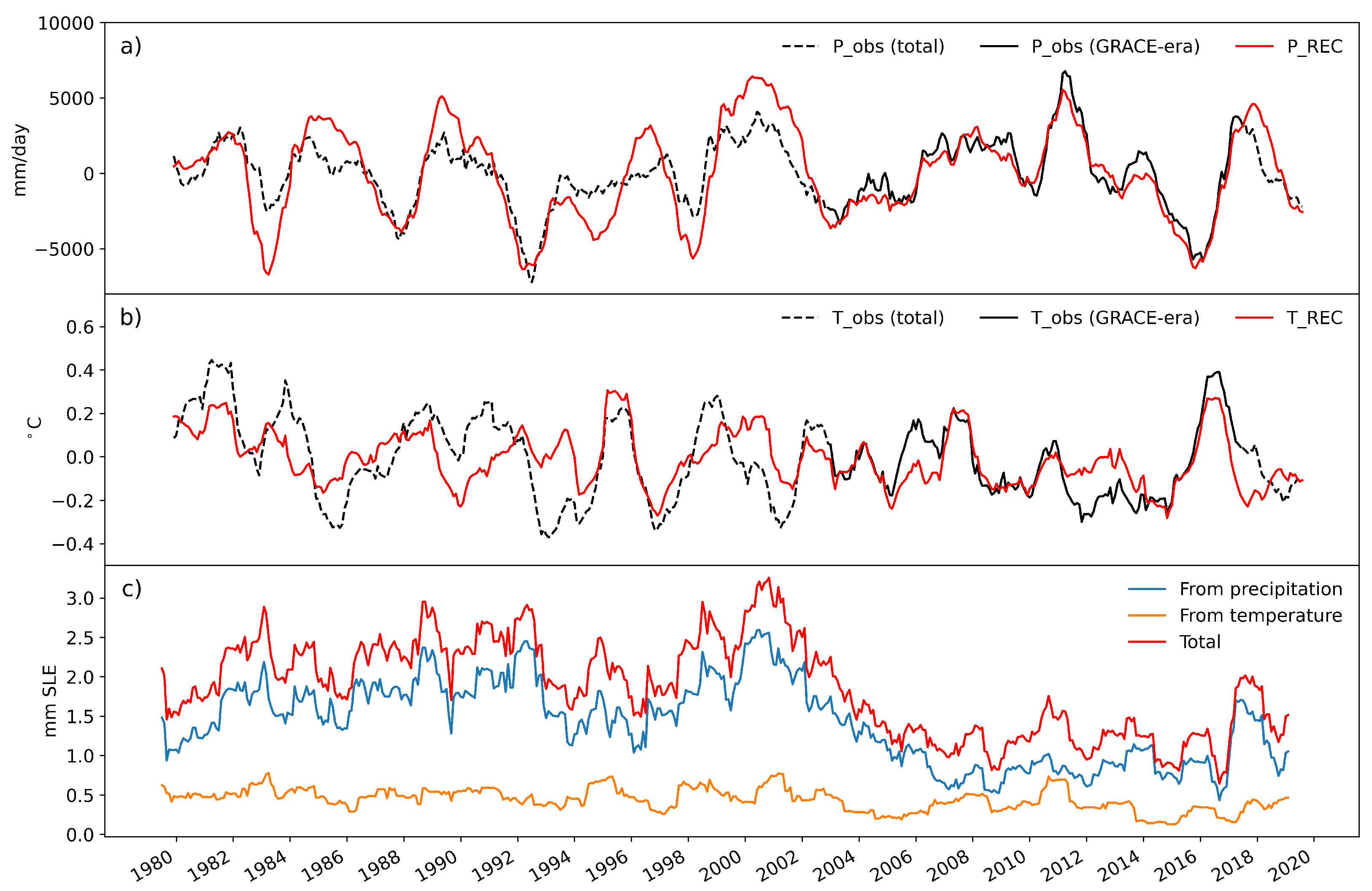
2.2.2. Reconstruction of Precipitation and Temperature Fields

In order to evaluate the consistency during the GRACE era with the pre-GRACE-era, we also reconstructed precipitation using the common modes in Section 2.2.1 Steps 1–3, and temperature following Step 5.

2.2.3. Uncertainty Estimation

Since GRACE was the first-ever and is still the only satellite mission to provide TWS estimates, there are no remote sensing-based observations to compare the TWS reconstructions. Large-scale in situ observations of TWS do not exist. Additionally, while land surface models have made considerable progress in recent years, they still have inadequate representations of TWS, and their TWS estimates are not quite reliable [30]. Considering all this, validating the TWS reconstruction for the pre-GRACE era is difficult.
Along with reconstruction of TWS, it is possible to use the common modes TWS shares with precipitation and temperature to reconstruct the latter two variables. In other words, exactly the same modes (or the physical processes that the modes represent) that were used for the TWS reconstruction could be also used in precipitation and temperature reconstructions. This provided a novel opportunity to validate the reconstructed modes: by comparing reconstructed precipitation and temperature data with their observational counterparts. Doing this gave a direct insight into how well could we expect the TWS reconstruction to behave for the pre-GRACE era.
The steps to compute uncertainty on the TWS reconstruction based on the above concept are as follows:
Step 1. Precipitation and temperature data were reconstructed following Section 2.2.2.
Step 2. A 12-month rolling root mean-square error (RMSE) was computed between the reconstructed precipitation and observed GPCP precipitation throughout the entire time duration (1979–2020).
Step 3. The resultant RMSE time series was then normalized by the average RMSE between reconstructed precipitation and observed precipitation during the the GRACE era.
Step 4. Average RMSE was computed between GRACE and the TWS reconstructed from common modes with precipitation (Step 3 from the Section 2.2.1).
Step 5. The average RMSE was then scaled to the normalized rolling RMSE time series from Step 3, to provide an estimate of the uncertainty on TWS reconstructed from precipitation (the blue curve in Figure 1c).
Step 6. Steps 2–5 were repeated for the reconstructed temperature data from Step 1, and an uncertainty estimate for the TWS reconstructed from temperature was obtained (the yellow curve in Figure 1c).
Step 7. The RMSE values from Steps 5 and 6 were added together to provide a total RMSE estimate for the reconstructed TWS.

3. Results

3.1. Uncertainty of the TWS Reconstruction

Figure 1a,b show global precipitation and temperature time series from observations and their reconstruction using the steps mentioned in Section 2.2.1 and Section 2.2.2. GRACE-era correlation coefficients ( ρ ) were 0.96 and 0.78 for precipitation and temperature model-observation comparisons, respectively. These correlations degraded by about 0.11 and 0.21 in the pre-GRACE era, with ρ being 0.85 and 0.57 for precipitation and temperature, respectively. This relative change in the model’s performance from the GRACE-era to the pre-GRACE era was used to estimate the uncertainty in the TWS reconstruction.
As can be seen in Figure 1c, the RMSE values of TWS reconstructed using precipitation are lowest during the GRACE era, and then increase as we go away from the GRACE era. The RMSE values, however, do not continue to increase as we go back in time, but decrease pre-2000 and become somewhat stable during 1981–1993. This is consistent with model-observation comparisons in Figure 1a,b. The reason behind this behavior is the contribution of the reconstructed modes to the total variance in observed precipitation. For example, in years where the RMSE is high, such as 2000–2002, precipitation is likely governed by some other modes that were not dominant during the GRACE era and hence are not represented in the reconstruction at all. In the low-RMSE periods, such as 1992–1999, the reconstructed modes indeed contributed significantly to the observed precipitation. The RMSEs of TWS reconstructed using temperature show overall stable behavior compared to precipitation. This suggests that the modes that were used to reconstruct TWS from temperature and the residual TWS contributed consistently throughout the 1980–2020 duration.
Overall, at the global scale, the uncertainty between TWS reconstruction and GRACE observations is 1.26 mm sea-level equivalents (mm SLE) for the GRACE era (with 0.92 and 0.34 mm SLE coming from the reconstructions using precipitation and temperature, respectively) and 2.26 mm SLE during the pre-GRACE era (with 1.75 and 0.51 mm SLE coming from the reconstructions from precipitation and temperature, respectively). It is worth noting that the uncertainty presented here concerns the model’s uncertainty alone. In other words, it describes the limits of the ability of our model to reconstruct the GRACE data. It does not include uncertainty and errors in the GRACE data. As a reference, 1 σ uncertainty of global TWS from GRACE is about 0.4 mm SLE [25,31].

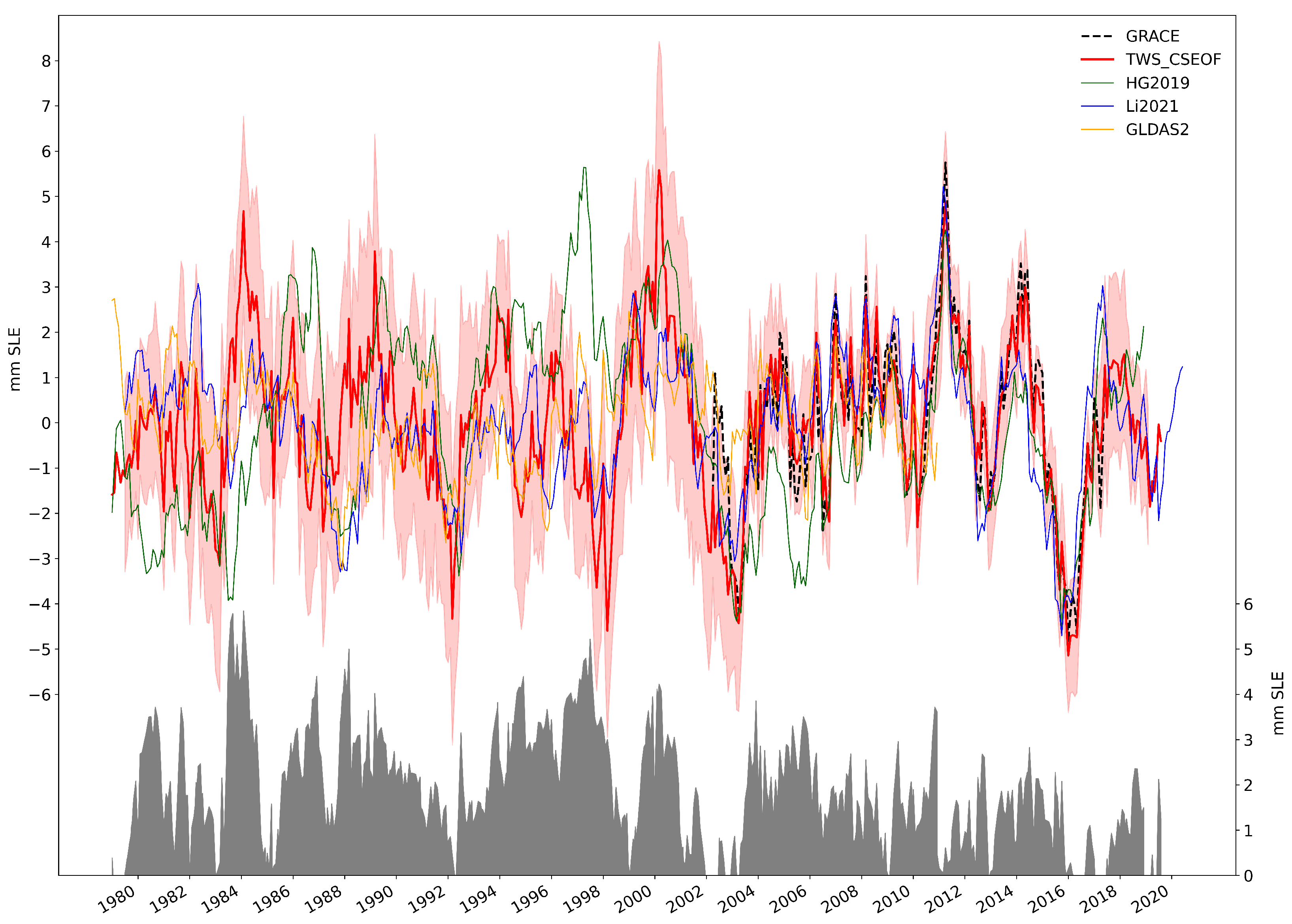
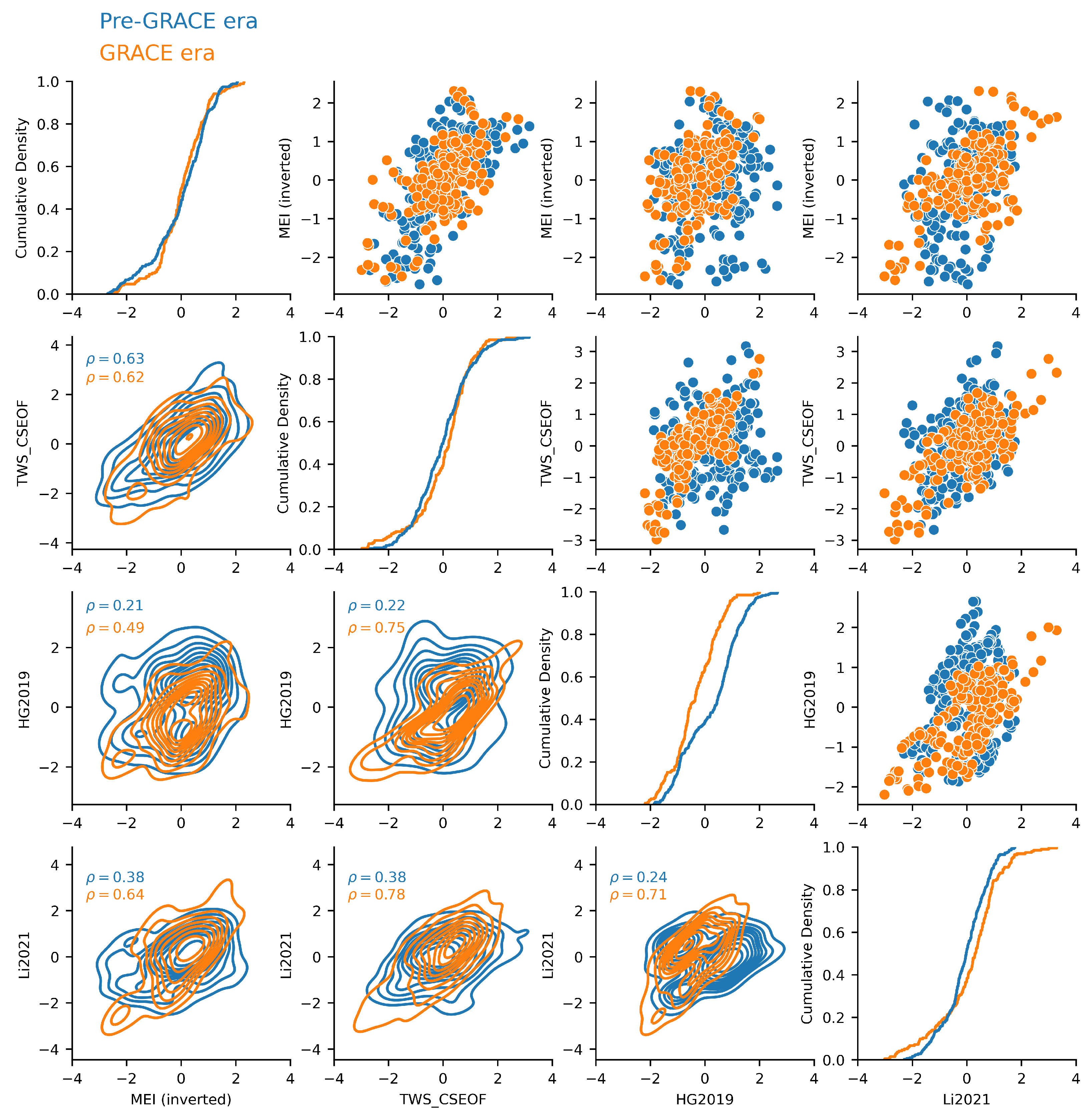
3.2. Global-Scale Analysis

Our aim for the TWS reconstruction was to optimize globally integrated TWS time series. Figure 2 shows the global TWS time series from various sources, such as GRACE, our reconstruction, GLDAS, and HG2019 and L2021. The long-term linear trend and the monthly climatology have been removed from these in order to focus on the interannual variability. As can be seen in the figure, the global TWS shows pronounced interannual variability that has a total range of about 12 mm SLE. Seen together, these curves correspond strongly with important ENSO years, such as the 1982–1983, 1997–1998, and 2014–2016 major El Niño events; and the 1998–2001 and 2010–2012 La Niña events.
While the TWS estimates, especially the reconstructions, agree quite well with GRACE data, as we go back in time, their differences increase. The gray shaded area in the figure shows the maximum spread between the curves at any given month. The spread is limited to about 3 mm SLE during the GRACE era but increases to up to 6 mm SLE in the pre-GRACE era.
To further understand the pre-GRACE-ra and GRACE-era behavior of the curves, in Figure 3 we analyze normalized distributions of the TWS estimates during these two eras and compare them to that of Multivariate ENSO Index Version 2 (MEI.v2) [28]. The diagonal panels describe empirical cumulative distribution functions (ECDF) of a single time series during the pre-GRACE and GRACE eras. In the top-left panel, it is shown that MEI behavior is similar in the pre-GRACE and GRACE eras, except for some lower ENSO values (El Niño years) in the GRACE era. Similarly, the TWS_CSEOF ECDFs from the two eras closely follow each other. The ECDFs for Li2021 show slightly different behavior for the two eras: less extreme values are present in the pre-GRACE era compared to the GRACE era. HG2019 shows remarkably different behavior during the two eras, with most differences occurring for the moderate values (neutral years) and positive extreme values (La Niña years).
Scatter and kernel density estimation (KDE) plots in the figure (above-diagonal and below-diagonal panels, respectively) each describe the relationship between a pair of time series broken into pre-GRACE and GRACE eras. Scatterplots show the actual values, whereas KDE plots show the density of the occurrences of certain values. Consistently with Figure 2, the scatter and KDE associations are stronger and positively correlated during the GRACE era (values in orange). Comparatively, the spread in the scatter is quite large during the pre-GRACE era (values in blue). Correlations with MEI are most consistent for TWS_CSEOF: pre-GRACE and GRACE era coefficients are 0.63 and 0.62, respectively. The correlations degrade rapidly in the pre-GRACE era for both HG2019 (from 0.49 to 0.21) and L2021 (from 0.63 to 0.37).

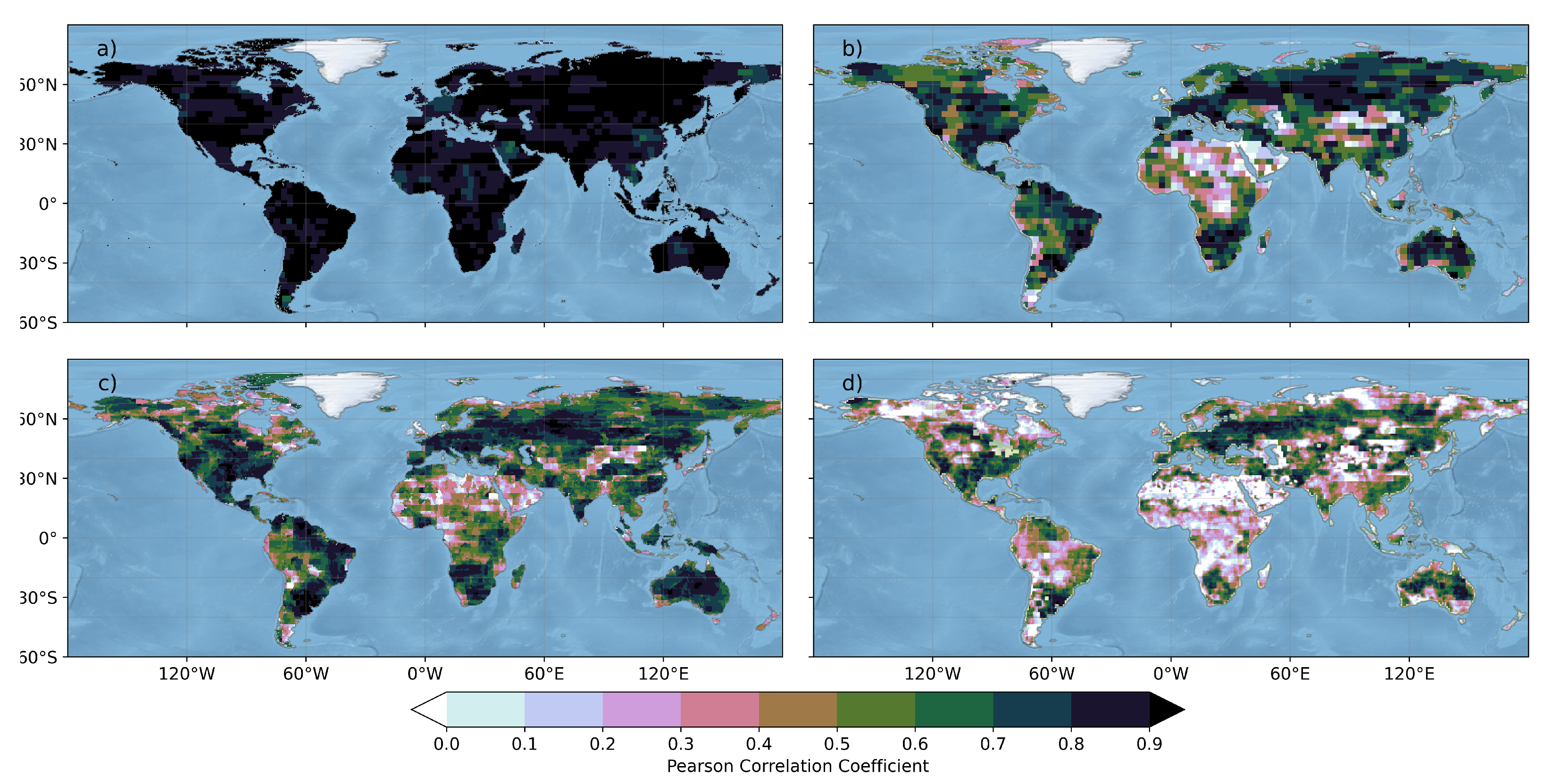
3.3. Local-Scale Analysis

While the aim of the reconstruction was to optimize the global time series, local-scale analysis brings insights into where the global signal comes from and highlights areas that are well or poorly represented by the reconstruction method.
Figure 4 shows detrended and de-seasonalized Pearson correlation coefficients between GRACE TWS observations and TWS_CSEOF, HG2019, Li2021, and GLDAS2. TWS_CSEOF has the highest correlation values (>0.8) consistently across most land regions. HG2019 and Li2021 have moderately high correlations for most land regions except in central and northern Africa and eastern Central Asia (encompassing parts of China and Mongolia). GLDAS2 has the lowest correlation values with GRACE compared to the three reconstructions, and these include parts of South America (including the Amazon basin) and South Asia.
While Figure 4 shows a favorable reconstruction-observation comparison during the GRACE era, it is important to understand how consistent this comparison would be in the pre-GRACE era. While direct comparison with gridded TWS observations is not possible for the pre-GRACE era, we provide comparisons between precipitation and temperature reconstructions and their observational counterparts. Figure 5 shows local Kolmogorov–Smirnov (K-S) goodness-of-fit test results between the input datasets of precipitation and temperature and their reconstructed counterparts (from Section 2.2.2) for the pre-GRACE era and the GRACE era. A low K-S statistic suggests that the two distributions are statistically identical and could have come from the same population.
The reconstruction-observation K-S statistics for precipitation (Figure 5a) and temperature (Figure 5c) are quite low for the GRACE era (mostly limited to 0.2), suggesting an excellent goodness-of-fit. For the pre-GRACE era (Figure 5b,d), the K-S statistic increases slightly by about 0.05 to 0.1 almost uniformly across most of the global land regions, which is still low overall (less than 0.3). In other words, comparing Figure 5a with Figure 5b and Figure 5c with Figure 5d shows that the model-observation distribution characteristics from the GRACE era were not significantly different in the pre-GRACE era.

4. Discussion

Through the analysis presented in Section 3, we try to address two main questions:
Question 1: “How good is the CSEOF method at reconstructing GRACE TWS, at global and local scales?”
Question 2: “Can the pre-GRACE era behavior of the TWS_CSEOF be expected to be consistent with its GRACE-era behavior, both globally and locally?”
Comparison against GRACE is crucial in addressing Question 1. The rationale is that, if our model were perfect, it would reproduce GRACE TWS perfectly. Based on Figure 2 and Figure 4, we can claim that our model performs quite well and compares favorably with GRACE observations at both global and local scales.
Addressing Question 2 is important, since it relates to the large spread that we see in the pre-GRACE era in Figure 2. It is also very challenging due to the lack of GRACE-like TWS observations in the past. We address this question in the following steps. First, we look at how the ENSO variability compares in the pre-GRACE and GRACE eras. After all, we specifically target interannual variability in our model, and numerous studies have well established that ENSO dominates TWS variability at the interannual time scale. The MEI ECDFs from Figure 3 suggest that the ENSO distributions are quite similar during the two eras; the KS-statistic is low, at D = 0.17. Next, we should note whether the ECDFs of our TWS reconstruction behave similarly in the pre-GRACE and GRACE eras. They do, and the KS-statistic is similarly low (D = 0.14). In addition to the ECDFs, we also compared correlations with MEI during pre-GRACE and GRACE eras. The scatter and kernel density plots in Figure 3 show an overall positive and narrow spread, and the correlation coefficients with MEI are identical for the pre-GRACE ( ρ = 0.63) and GRACE ( ρ = 0.62) eras. Overall, this suggests that globally, the TWS_CSEOF behavior during pre-GRACE and GRACE eras is consistent and similar to that of ENSO variability.
While ENSO variability serves as a reasonable proxy for interannual variability in global TWS and enables cross-checking the pre-GRACE-era and GRACE-era behavior of TWS_CSEOF, no such data are readily available at local scales. We addressed this problem by making use of the CSEOF method itself, which, along with TWS reconstruction, can also reconstruct the precipitation and temperature datasets. Since the three reconstructions were based on exactly the same modes, a direct comparison can be made between precipitation and temperature reconstructions and their observational counterparts during pre-GRACE and GRACE eras. The differences highlight regions where our TWS_CSEOF reconstruction can be expected to perform consistently during the pre-GRACE era, and where its reliability may degrade. Comparing Figure 5a,b suggests that the distribution of the reconstructed precipitation is close to that of the observed precipitation for both pre-GRACE and GRACE periods, especially in the high-precipitation regions, such as the rain forests and monsoon regions, whereas the model’s performance is degraded a bit in the arid regions, such as northeast Africa and the Persian Gulf states, in the pre-GRACE era. Similarly, comparing Figure 5c,d suggests that the reconstructed temperatures also closely match the distribution of the observed temperatures for both eras. This is especially true in regions where the temperature has a close link with TWS, viz., the northern higher latitudes. In the case of both variables, the model degradation during the pre-GRACE era is limited to a roughly 0.1 increase in the KS statistic D over most regions. In other words, the probability that the two distributions are different is about 10% higher in the pre-GRACE era. However, the overall probability of the distributions being different is still less than 30% (D statistic is less than 0.3) over most land regions. Overall, Figure 5 suggests that the local relationships between model-observations are quite consistent during the pre-GRACE and GRACE eras for most of the global land area.
Finally, another challenge in TWS reconstruction was to compute a realistic uncertainty value for our model. By comparing how the precipitation and temperature reconstructions—from exactly the same modes as their corresponding TWS reconstructions—compare with the observations in the pre-GRACE era, one can understand how the model could deviate from the observations in the pre-GRACE era. In Figure 1, low RMSE values during the GRACE era are not surprising and provide an estimate of how good the model is with its optimal settings. However, the RMSE values can be seen to increase as we go away from the GRACE era, suggesting model degradation. However, the model does not continue to degrade further and in fact improves during certain years, when the modes used to reconstruct the variability contribute more to the total variance. There are also certain periods when the RMSE is quite high, such as 2000–2002. Interestingly, these are also the periods when most of the reconstruction data do not agree with each other.

5. Conclusions

In this study, noting the large spread among the TWS reconstruction datasets in estimating global land TWS variability, especially in the pre-GRACE era, we applied a novel method of CSEOF to estimate TWS. We found the resultant reconstruction (TWS_CSEOF) performs quite well globally and locally against GRACE. Doing extensive tests on its consistency during the pre-GRACE era, we found that the TWS variability remains consistent with the GRACE-era data, both at global and local scales. We also provided a realistic, time-varying uncertainty estimate of the TWS reconstruction based on the contribution of the CSEOF modes to the total variance back in time. The reconstructed TWS is likely useful for a range of stakeholders. For example, globally-integrated TWS reconstruction that is consistent with ENSO variability can be used readily by the global sea-level community in constraining the global means sea-level budget, e.g., [6]. The reconstructed TWS, being based on temperature and precipitation relationships with TWS, excludes direct signals from human water management. Thus, regional/local hydrologists, water managers and policymakers may find it useful for providing estimates of the interannual climatic variability in their regional/local water resources. Finally, while the reconstructed TWS was not optimized to fill the GRACE/GRACE-Follow On gap, it can certainly be used for that purpose. Further analysis of the contributing modes could provide insight into the climatic drivers of the interannual-to-decadal variability in terrestrial water storage.

Author Contributions

H.A.C., B.D.H. and J.T.R. together developed the concept based on B.D.H.’s previous studies. B.D.H. developed the initial method and finalized it with discussions with H.A.C. and J.T.R.; H.A.C. conducted tests and validation analysis and wrote the text under the guidance from J.T.R.; B.D.H. contributed heavily to the methods section. All authors contributed to improving the analysis and presentation of the results. All authors have read and agreed to the published version of the manuscript.

Funding

Funding was provided by the NASA GRACE-FO Science Team. This work was performed at the Jet Propulsion Laboratory, California Institute of Technology, under contract with NASA.

Data Availability Statement

The resultant TWS reconstruction from this study is available for download at https://doi.org/10.5281/zenodo.6659543.

Conflicts of Interest

The authors declare no conflict of interest.

References

  1. Tapley, B.; Watkins, M.; Flechtner, F.; Reigber, C.; Bettadpur, S.; Rodell, M.; Sasgen, I.; Famiglietti, J.; Landerer, F.; Chambers, D.; et al. Contributions of GRACE to understanding climate change. Nat. Clim. Chang. 2019, 5, 358–369. [Google Scholar] [CrossRef] [PubMed]
  2. Landerer, F.W.; Flechtner, F.M.; Save, H.; Webb, F.H.; Bandikova, T.; Bertiger, W.I.; Bettadpur, S.V.; Byun, S.H.; Dahle, C.; Dobslaw, H.; et al. Extending the Global Mass Change Data Record: GRACE Follow-On Instrument and Science Data Performance. Geophys. Res. Lett. 2020, 47. [Google Scholar] [CrossRef]
  3. Rodell, M.; Beaudoing, H.K.; L’ecuyer, T.; Olson, W.S.; Famiglietti, J.S.; Houser, P.R.; Adler, R.; Bosilovich, M.G.; Clayson, C.A.; Chambers, D.; et al. The observed state of the water cycle in the early twenty-first century. J. Clim. 2015, 28, 8289–8318. [Google Scholar] [CrossRef] [Green Version]
  4. L’Ecuyer, T.S.; Beaudoing, H.K.; Rodell, M.; Olson, W.; Lin, B.; Kato, S.; Clayson, C.A.; Wood, E.; Sheffield, J.; Adler, R.; et al. The Observed State of the Energy Budget in the Early Twenty-First Century. J. Clim. 2015, 28, 8319–8346. [Google Scholar] [CrossRef] [Green Version]
  5. Humphrey, V.; Zscheischler, J.; Ciais, P.; Gudmundsson, L.; Sitch, S.; Seneviratne, S.I. Sensitivity of atmospheric CO2 growth rate to observed changes in terrestrial water storage. Nature 2018, 560, 628–631. [Google Scholar] [CrossRef] [PubMed]
  6. Hamlington, B.D.; Piecuch, C.G.; Reager, J.T.; Chandanpurkar, H.; Frederikse, T.; Nerem, R.S.; Fasullo, J.T.; Cheon, S.H. Origin of interannual variability in global mean sea level. Proc. Natl. Acad. Sci. USA 2020, 117, 13983–13990. [Google Scholar] [CrossRef]
  7. Humphrey, V.; Gudmundsson, L. GRACE-REC: A reconstruction of climate-driven water storage changes over the last century. Earth Syst. Sci. Data 2019, 11, 1153–1170. [Google Scholar] [CrossRef] [Green Version]
  8. Li, F.; Kusche, J.; Chao, N.; Wang, Z.; Löcher, A. Long-Term (1979–Present) Total Water Storage Anomalies over the Global Land Derived by Reconstructing GRACE Data. Geophys. Res. Lett. 2021, 48. [Google Scholar] [CrossRef]
  9. Sun, Z.; Long, D.; Yang, W.; Li, X.; Pan, Y. Reconstruction of GRACE Data on Changes in Total Water Storage Over the Global Land Surface and 60 Basins. Water Resour. Res. 2020, 56. [Google Scholar] [CrossRef]
  10. Sun, A.Y.; Scanlon, B.R.; Save, H.; Rateb, A. Reconstruction of GRACE Total Water Storage Through Automated Machine Learning. Water Resour. Res. 2021, 57. [Google Scholar] [CrossRef]
  11. Yu, Q.; Wang, S.; He, H.; Yang, K.; Ma, L.; Li, J. Reconstructing GRACE-like TWS anomalies for the Canadian landmass using deep learning and land surface model. Int. J. Appl. Earth Obs. Geoinf. 2021, 102, 102404. [Google Scholar] [CrossRef]
  12. Yang, X.; Tian, S.; You, W.; Jiang, Z. Reconstruction of continuous GRACE/GRACE-FO terrestrial water storage anomalies based on time series decomposition. J. Hydrol. 2021, 603, 127018. [Google Scholar] [CrossRef]
  13. Mo, S.; Zhong, Y.; Forootan, E.; Mehrnegar, N.; Yin, X.; Wu, J.; Feng, W.; Shi, X. Bayesian convolutional neural networks for predicting the terrestrial water storage anomalies during GRACE and GRACE-FO gap. J. Hydrol. 2022, 604, 127244. [Google Scholar] [CrossRef]
  14. Boening, C.; Willis, J.K.; Landerer, F.W.; Nerem, R.S.; Fasullo, J. The 2011 La Niña: So strong the oceans fell. Geophys. Res. Lett. 2012, 39. [Google Scholar] [CrossRef] [Green Version]
  15. Fasullo, J.T.; Boening, C.; Landerer, F.W.; Nerem, R.S. Australia’s unique influence on global sea level in 2010–2011. Geophys. Res. Lett. 2013, 40, 4368–4373. [Google Scholar] [CrossRef]
  16. Cheon, S.H.; Hamlington, B.D.; Reager, J.T.; Chandanpurkar, H.A. Identifying ENSO-related interannual and decadal variability on terrestrial water storage. Sci. Rep. 2021, 11, 13595. [Google Scholar] [CrossRef]
  17. Piecuch, C.G.; Quinn, K.J. El Niño La Niña, and the global sea level budget. Ocean. Sci. 2016, 12, 1165–1177. [Google Scholar] [CrossRef] [Green Version]
  18. Kim, K.Y.; Hamlington, B.; Na, H. Theoretical foundation of cyclostationary EOF analysis for geophysical and climatic variables: Concepts and examples. Earth-Sci. Rev. 2015, 150, 201–218. [Google Scholar] [CrossRef] [Green Version]
  19. Kim, K.Y.; North, G.R.; Huang, J. EOFs of one-dimensional cyclostationary time series: Computations, examples, and stochastic modeling. J. Atmos. Sci. 1996, 53, 1007–1017. [Google Scholar] [CrossRef]
  20. Hamlington, B.; Leben, R.; Nerem, R.; Han, W.; Kim, K.Y. Reconstructing sea level using cyclostationary empirical orthogonal functions. J. Geophys. Res. Ocean. 2011, 116, 12015. [Google Scholar] [CrossRef]
  21. Strassburg, M.; Hamlington, B.; Leben, R.; Kim, K.Y. A comparative study of sea level reconstruction techniques using 20 years of satellite altimetry data. J. Geophys. Res. Ocean. 2014, 119, 4068–4082. [Google Scholar] [CrossRef] [Green Version]
  22. Hamlington, B.; Leben, R.; Kim, K.Y. Improving sea level reconstructions using non-sea level measurements. J. Geophys. Res. Ocean. 2012, 117, 11364. [Google Scholar] [CrossRef] [Green Version]
  23. Hamlington, B.; Reager, J.; Chandanpurkar, H.; Kim, K.Y. Amplitude modulation of seasonal variability in terrestrial water storage. Geophys. Res. Lett. 2019, 46, 4404–4412. [Google Scholar] [CrossRef]
  24. Watkins, M.M.; Wiese, D.N.; Yuan, D.N.; Boening, C.; Landerer, F.W. Improved methods for observing Earth’s time variable mass distribution with GRACE using spherical cap mascons. J. Geophys. Res. Solid Earth 2015, 120, 2648–2671. [Google Scholar] [CrossRef]
  25. Wiese, D.N.; Landerer, F.W.; Watkins, M.M. Quantifying and reducing leakage errors in the JPL RL05M GRACE mascon solution. Water Resour. Res. 2016, 52, 7490–7502. [Google Scholar] [CrossRef]
  26. Adler, R.F.; Huffman, G.J.; Chang, A.; Ferraro, R.; Xie, P.P.; Janowiak, J.; Rudolf, B.; Schneider, U.; Curtis, S.; Bolvin, D.; et al. The Version-2 Global Precipitation Climatology Project (GPCP) Monthly Precipitation Analysis (1979–Present). J. Hydrometeorol. 2003, 4, 1147–1167. [Google Scholar] [CrossRef]
  27. Hersbach, H.; Bell, B.; Berrisford, P.; Hirahara, S.; Horányi, A.; Muñoz-Sabater, J.; Nicolas, J.; Peubey, C.; Radu, R.; Schepers, D.; et al. The ERA5 global reanalysis. Q. J. R. Meteorol. Soc. 2020, 146, 1999–2049. [Google Scholar] [CrossRef]
  28. Zhang, T.; Hoell, A.; Perlwitz, J.; Eischeid, J.; Murray, D.; Hoerling, M.; Hamill, T.M. Towards Probabilistic Multivariate ENSO Monitoring. Geophys. Res. Lett. 2019, 46, 10532–10540. [Google Scholar] [CrossRef]
  29. Rodell, M.; Houser, P.; Jambor, U.; Gottschalck, J.; Mitchell, K.; Meng, C.J.; Arsenault, K.; Cosgrove, B.; Radakovich, J.; Bosilovich, M.; et al. The global land data assimilation system. Bull. Am. Meteorol. Soc. 2004, 85, 381–394. [Google Scholar] [CrossRef] [Green Version]
  30. Scanlon, B.; Zhang, Z.; Save, H.; Sun, A.; Müller, S.H.; van, B.L.; Wiese, D.; Wada, Y.; Long, D.; Reedy, R.; et al. Global models underestimate large decadal declining and rising water storage trends relative to GRACE satellite data. Proc. Natl. Acad. Sci. USA 2018, 115, E1080–E1089. [Google Scholar] [CrossRef]
  31. Chandanpurkar, H.A.; Reager, J.T.; Famiglietti, J.S.; Nerem, R.S.; Chambers, D.P.; Lo, M.H.; Hamlington, B.D.; Syed, T.H. The Seasonality of Global Land and Ocean Mass and the Changing Water Cycle. Geophys. Res. Lett. 2021, 48. [Google Scholar] [CrossRef]
Figure 1. Time series of global terrestrial precipitation (a) and 2 m air temperature (b) along with their reconstructions (P_REC and T_REC, respectively), and the uncertainty of the reconstructed global TWS (TWS_CSEOF) based on precipitation and temperature (c).
Remotesensing 14 05677 g001
Figure 2. Detrended and deseasonalized time series of global TWS from GRACE, TWS_CSEOF, HG2019, Li2021, and GLDAS2. The shaded red area indicates uncertainty on the TWS_CSEOF time series. The gray area at the bottom depicts the maximum spread between all the curves at any given month.
Remotesensing 14 05677 g002
Figure 3. A series of pair plots showing normalized distributions of global TWS from TWS_CSEOF, HG2019, Li2021, and the Multivariate ENSO Index. The diagonal panels show ECDFs, the above-diagonal panels show scatter plots, and the below-diagonal panels show 2D kernel density estimation. The colors indicate the periods of the time series (pre-GRACE-era and GRACE era).
Remotesensing 14 05677 g003
Figure 4. Correlations with GRACE for TWS_CSEOF (a), HG2019 (b), Li2021 (c), and GLDAS2 (d).
Remotesensing 14 05677 g004
Figure 5. Kolmogorov—Smirnov goodness-of-fit statistic D between reconstructed and GPCP precipitation during the GRACE era (a) and pre-GRACE-era (b), and between reconstructed and ERA5 temperature during the GRACE era (c) and pre-GRACE-era (d).
Remotesensing 14 05677 g005
Publisher’s Note: MDPI stays neutral with regard to jurisdictional claims in published maps and institutional affiliations.

