Abstract
The availability of low-cost microwave components today enables the development of various high-frequency sensors and radars, including Ground-based Synthetic Aperture Radar (GBSAR) systems. Similar to optical images, radar images generated by applying a reconstruction algorithm on raw GBSAR data can also be used in object classification. The reconstruction algorithm provides an interpretable representation of the observed scene, but may also negatively influence the integrity of obtained raw data due to applied approximations. In order to quantify this effect, we compare the results of a conventional computer vision architecture, ResNet18, trained on reconstructed images versus one trained on raw data. In this process, we focus on the task of multi-label classification and describe the crucial architectural modifications that are necessary to process raw data successfully. The experiments are performed on a novel multi-object dataset RealSAR obtained using a newly developed 24 GHz (GBSAR) system where the radar images in the dataset are reconstructed using the Omega-k algorithm applied to raw data. Experimental results show that the model trained on raw data consistently outperforms the image-based model. We provide a thorough analysis of both approaches across hyperparameters related to model pretraining and the size of the training dataset. This, in conclusion, shows how processing raw data provides overall better classification accuracy, it is inherently faster since there is no need for image reconstruction and it is therefore useful tool in industrial GBSAR applications where processing speed is critical.
1. Introduction
Synthetic Aperture Radar (SAR) technology is crucial in many modern monitoring applications where optical images are not sufficient or restrictions in terms of light conditions or cloud coverage play a major role. To reach adequate resolution the antenna-based radar system should have a large sensor antenna. The resolution of an optical image obtained using the Sentinel-2 satellite with a mean orbital altitude of 786 km is around 20 m [1]. In order to achieve an equal resolution using a C-band sensor (common in SAR satellites) from that altitude, the sensor antenna would have to be over 2 km long, which is not practical. To virtually extend (synthesize) the length of the antenna (or antenna array), SAR concept utilizes sensor’s movement to combine data acquired from multiple positions and reconstruct radar image of the observed area. In the Sentinel-1 SAR satellite launched in 2014, the movement of the 12.3-m-long antenna provides coverage of a 400 km wide area with a spatial resolution of 5 m [1].
The same principle can be applied in a terrestrial remote sensing imaging system—Ground-based SAR (GBSAR). The main concept of GBSAR is based on the sensor antenna which radiates perpendicular to the moving path, but the sensor moves along a ground track, covering the area in front of it. Even though, in many applications, distances between sensors and observed objects can be up to several kilometers, a smaller distance in combination with wider frequency bandwidth can be interesting for sensing small deformations. Satellite frequencies above the X band are rarely used in SAR due to absorption. However, since that is not a strict limitation for terrestrial GBSAR, higher frequencies and wider bandwidths can be used to achieve higher resolutions in radar images, which is essential for anomaly detection and small object recognition.
Such images, in combination with machine learning algorithms, enable surface deformation monitoring [2,3,4,5,6], snow avalanche identification [7], bridge [8] and dam structure monitoring [9], open pit mine safety management [10], and terrain classification [11]. Moreover, machine learning enables object classification using only radar images. Applications include the classification of military targets from the MSTAR dataset [12,13,14,15,16,17,18,19], ship detection [20,21,22,23,24], and subsurface object classification with an ultra-wideband GBSAR [25]. Radars with 32–36 GHz and 90–95 GHz frequency bands have been shown to accurately locate small metallic targets in the near-field region [26]. To facilitate deep learning research for SAR data, LS-SSDD-v1.0 [27], a dataset for small ship detection from SAR images was released, together with many standardized baselines. This resulted in subsequent advances in deep learning methods for ship classification [28,29], detection [30], and instance segmentation [31,32] in SAR images.
On the other hand, object classification on GBSAR data has not been explored sufficiently since most of the aforementioned work was focused on solving problems encountered in typical GBSAR applications. The potential of GBSAR systems lies in industrial applications, such as monitoring and object detection in harsh environments, and classification of concealed objects. We perform object classification on two modalities of GBSAR data: images reconstructed using the Omega-K algorithm and raw GBSAR data. Both approaches are based on a popular convolutional neural network (CNN) architecture—ResNet18—with certain modifications to accommodate processing raw GBSAR data.
A crucial part of the image reconstruction algorithm is an approximation step, which negatively influences the integrity of the data. We tested and quantified its impact on classification results by comparing multiple models based on raw and reconstructed GBSAR data. The idea of using raw GBSAR data is similar to various end-to-end learning approaches [33], which became more prevalent with the advent of deep learning. In such a paradigm, the model implicitly learns optimal representations of raw data [34], without any explicit transformations during data preprocessing.
The rest of the paper is organized as follows: Section 2 introduces the theory behind GBSAR and the radar image reconstruction algorithm. It also covers the implementation used in generating measurement sets presented in Section 3. Section 4 describes relevant deep learning concepts, such as feature engineering, end-to-end learning, and multi-label classification. It describes two concrete approaches to address GBSAR object classification, which correspond to the two input modalities. The experimental setup and evaluation results are described and analyzed in Section 5. Further discussions and interpretations are given in Section 6. Section 7 provides conclusions and future work.
2. Gbsar Theory and Implementation
2.1. GBSAR
The main idea of GBSAR is, following SAR concept, to virtually extend sensor antenna by utilizing sensor movement along the set track while it emits and receives EM waves. The set of measurements provides extraction of the distances to the observed object in each sensor position and, consequently, radar image reconstruction. Range and azimuth resolution of the radar image are mostly determined by the sensor frequency bandwidth and length of the used track, respectively. Hence, wider bandwidth and longer track (for example some sort of rail) provide better range and azimuth resolution [35].
There are two operational modes regarding sensor movement: continuous and stop-and-go mode. In the first one sensor moves with constant speed from start to the end of the used rail, while in the second one sensor movement is paused at each sampling position to acquire data without impact of motion. In stop-and-go mode step size and total aperture length can be precisely set but it should be emphasized that chosen values affect azimuth resolution. In both modes, the moving sensor has to repeatedly provide information about distance which is commonly obtained by using Frequency Modulated Continuous Wave (FMCW) radar principle as the base radar system due to its relatively simple and well known implementation.
FMCW radar radiates continuous signal whose operating frequency changes during transmission. Operating frequency sweeps through some previously defined frequency band B with a known function which is usually linear (most commonly sawtooth type function is used [36]). The same frequency sweep is observed in the echo or received signal which is delayed in time for the time required by the signal to travel to the object and be reflected back. Emitted and received signals are then mixed in order to eliminate high-frequency content in the received signal and use the low frequency difference to extract the delay in the received signal. To provide the analytical basis we start with a typical sawtooth wave which is made of periodic repetition (period T) of upchirp (frequency increases) or downchirp (frequency decreases) signals. Upchirp’s frequency changes according to the linear function with rate of change equal to . Carrier frequency is denoted by . In the complex form, emitted signal is given by the function
Received signal is delayed in time for the time it takes the signal to travel to the observed object and returns back. Geometry of a standard GBSAR system and position of the object are described in Figure 1. Time delay between the transmission and detection is denoted by ,
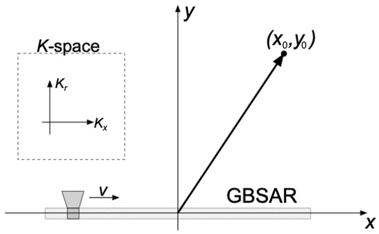
Figure 1.
Ground-based SAR geometry. Coordinates represent position of a point object in real space. In the dashed square, coordinates of the Fourier domain space or K-space are presented. is a wave vector coordinate in the range direction while is a wave vector coordinate in the x direction.
After the mixing process we obtain signal S without high-frequency content
All information about the observed object, that can be extracted by radar, is stored in the signal S and reconstruction algorithms operate directly on the signal S. Signal S can be interpreted in various different ways and the algorithm used for the reconstruction depends on the interpretation of S. Using Fourier transform in the spatial domain signal S can be interpreted as the spatial spectrum in azimuthal and distance variables [37].
Position of the object is saved in the and coordinates in the first two complex exponential functions. Coordinates are multiplied by wave vector variables and . Third exponential function is a residual of a finite recording step size and finite radar’s bandwith B. It manifests through the parameter in the Fourier domain. Radar moves with a constant speed v, c is a speed of light and represents chirp’s rate of change.
We note that this is only one of many ways of interpreting signal S and the choice of reconstruction algorithm depends on this interpretation. This kind of interpretation leads to frequency domain reconstruction algorithms. Time domain algorithms usually have higher algorithm complexity but are more robust to the sensor irregular movement during radar operation [38].
2.2. Image Reconstruction
Image reconstruction algorithms are used to generate radar image from the signal S. In this work, signals were recorded using GBSAR radar which operates in the stop-and-go mode. Received signal will be interpreted according to (3) and image reconstruction will be based on Omega-K algorithm [39]. This algorithm has many different implementations for images generated by GBSAR [37,40], but the main idea of these types of algorithms is to apply several processing steps on the spatial spectrum and then use inverse Fourier transform in order to extract position of the object.
Spatial spectrum (4) can be interpreted as a product of several functions carrying information about the object and information about various side effects of SAR radar acquisition. The task of the Omega-K algorithm is to separate those two parts and filter information about side effects out. Second part of the spatial spectrum S,
represents residual frequency modulation due to finite step between two image acquisition. If we filter out this part then the remaining part of the spatial spectrum contains information about spatial coordinates of the object
which can be extracted using the inverse Fourier transform. It gives , or object position. Constant
does not affect image reconstruction process.
Every Omega-K algorithm is a discrete implementation of previously described steps. They differ by the way they treat spatial spectrum S in order to separate information about position of the object from various side effects of image acquisition. They usually have part for the residual frequency modulation compensation, interpolation from spherical to Cartesian coordinate system and they end with 2D inverse Fourier transform (2D IFFT).
Reconstruction algorithms are used in order to recreate captured image according to predefined signal model, such as (3). Ideally, reconstruction algorithms take signal S and reproduce the image of the observed object without the loss of information in the signal S. In reality, all those steps necessarily introduce an error in the reconstruction process and affect the information in S. Numerical algorithms, such as FFT, have very well known and well-described numerical error and those steps do not affect information in S significantly. On the other side, approximations, such as frequency modulation compensation, residual-phase compensation, and interpolation from spherical to Cartesian coordinate system, are approximation steps associated to the predefined signal model. Algorithms used in those steps are not as researched as the FFT algorithm is, they are not implemented in numerical libraries, and they necessarily degrade the information in S as a result of their approximation character [37]. Although it is easier for human beings to notice useful information and recognize captured object in the reconstructed image than it is in the raw data, it does not mean that there is more information in the reconstructed image. As is described before, just the opposite is true due to all approximation algorithms. Reconstructed representation of the signal S is just easier for human beings to grasp than the raw data. That means that a neural network based classifier, that operates directly on the raw data, has a significant potential for a higher accuracy than the classifier that operates on the reconstructed images.
2.3. Implementation
In order to obtain radar images of objects from the ground while keeping flexibility regarding step size, total aperture length, polarization, and observing angle, GBSAR named GBSAR-Pi was developed. It is based on Raspberry Pi 4B (RPi) microcomputer that controls voltage controlled oscillator (VCO) in FMCW module Innosent IVS-362 [41]. The module operates in 24 GHz band and, besides VCO, has integrated trasmitting and receiving antenna, and mixer. The mechanical platform which contains RPi with AD/DA converter, FMCW module and amplifier is tailor 3D printed to enable precise linear movement and change of polarization. Polarization can be manually set to horizontal (HH) or vertical (VV). Movement of the platform is provided by 5V stepper motor. Figure 2 shows developed GBSAR-Pi: on one side of 1.2 m long rail track is stepper motor which is controlled by the RPi located in the movable white 3D printed platform. The platform also contains FMCW module on the front and touch-screen display used for measurement parameter setup, monitoring, and ultimately representation of reconstructed radar image.
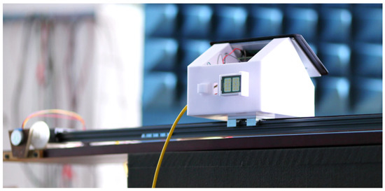
Figure 2.
Developed GBSAR-Pi.
Developed GBSAR-Pi works in stop-and-go mode. The process of obtaining measurement for one radar image is following: RPi over DA converter controls VCO on FMCW module to emit upchirp signals using pin, as shown in Figure 3. The module in each step transmits and receives signals, mixes them, and the resultant signal in low frequency band is sent to the microcomputer over In phase pin (IF1 in Figure 3) and AD converter. In order to maximize SNR, in each step the system emits multiple signals and stores the average of received ones. When the result is stored, RPi runs stepper motor via four control pins to move the platform for one step of previously set size. The enable pin in Figure 3 is used to switch off the power supply of the VCO. The process continues until it reaches last step. After that obtained matrix of average signals from each step is stored locally and sent to the server.
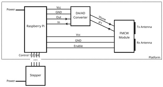
Figure 3.
GBSAR-Pi scheme.
FMCW signals transmitted by the module have central frequency of 24 GHz and sweep range is set to 700 MHz bandwidth. Hence, from well known equation for FMCW range resolution , the used bandwidth provides range resolution of the system cm. Each sweep in emitted signal is generated by RPi with 1024 frequency points and has a duration of 166 ms which gives chirp rate change of frequency . Signal stored in each step is average of 10 received signals. FMCW module has output power (EIRP) 12.7 dBm. Number of steps and step size are adjustable and in our measurements there were two cases: case of 0.4 cm step size and 160 steps, and 1 cm step size and 30 steps case. Antennas polarization can be changed manually by rotating case with FMCW module set on the front side of the platform. Since the antennas are integrated within the module, the system is limited to HH and VV polarizations only. GBSAR-Pi use two battery sources: first one charges RPi, AD/DA converter and FMCW module, and second one stepper motor. The whole system is, thus, fully autonomous with the system being controlled by display set on the platform and optionally an external keyboard.
Following Section 2.2, image reconstruction algorithm Omega-K was implemented using python programming language and additional libraries numpy and scipy. Regarding the algorithm, most important methods of the implementation are numpy FFT (Fast Fourier Transform) and IFFT (Inverse FFT), and scipy interpolate which provides one-dimensional array interpolation (interp1d). The visualization of a reconstructed radar image was accomplished using libraries matplotlib (pyplot) and seaborn (heatmap). Implementation consists of following steps: Hilbert transform, RVP (Residual Video Phase), Hanning window, FFT, Reference function multiply (RFM), interpolation, IFFT, and visualization. Complete program code with adjustable central frequency, bandwidth, chirp duration, and step size is given in [42].
3. Data Acquisition
3.1. Measurements
The measurements were taken using GBSAR-Pi. There were two sets of measurements: the first was conducted in laboratory conditions, while the second set of measurements was obtained in a more complex “real world” environment. Thus, we named the collected datasets LabSAR and RealSAR, respectively.
In LabSAR, three test objects set at the same position in an anechoic chamber are recorded. The test objects were a big metalized box, a small metalized box, and a cylindrical plastic bottle filled with water. Hence, the objects were different in size and material reflectance. The distance between GBSAR-Pi and the observed object did not change between measurements and was approximately 1 m. The azimuth position of the object was at the center of the GBSAR-Pi rail track. Only one object was recorded in each measurement for this setup. All measurements were conducted using horizontal polarization. 160 steps of size 4 mm gave total aperture length of 64 cm.
In RealSAR, the conditions were not as ideal. The measurements were intentionally conducted in a room full of various objects in order to produce additional noise. Once again, there were three test objects. However, the objects were empty bottles of similar size and shape. The bottles could be distinguished based on the different reflectances of the material. The three bottles used as test objects were made from aluminium, glass, and plastic. Compared to LabSAR, there was much more variance in recorded scenes since any of the eight () possible subsets of three objects could appear in a given scene (including an empty scene without any objects). Moreover, the different object positions, which vary in both azimuth and range direction, and different polarizations used for recording also contribute to the complexity of the task. We note that any scene can include at most one object of a certain material. Compared to LabSAR, the step size was increased to 1 cm, while the total aperture length was decreased to 30 cm. RealSAR objects are shown in Figure 4. Comparison between measurement sets is given in Table 1.
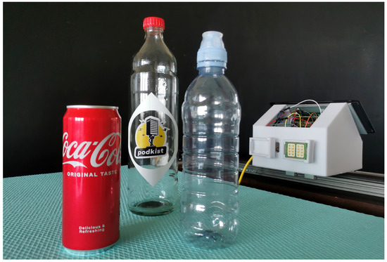
Figure 4.
RealSAR objects: aluminium, glass and plastic bottle, and GBSAR-Pi.

Table 1.
LabSAR and RealSAR measurement set comparison. First five rows describe objects and scenes, while others GBSAR-Pi parameters used in the measurements.
3.2. Datasets
Using the measurement sets LabSAR and RealSAR, four datasets were created: LabSAR-RAW, LabSAR-IMG, RealSAR-RAW, and RealSAR-IMG. LabSAR-RAW and RealSAR-RAW consist of raw data from measurement sets mentioned in their names. At the same time, LabSAR-IMG and RealSAR-IMG contain radar images generated using the reconstruction algorithm on that raw data. Since the number of frequency points in GBSAR-Pi did not change throughout the measurements, the dimensions of matrices in RAW datasets depend only on the number of steps: in LabSAR-RAW, each matrix is 160 × 1024, while in RealSAR-RAW, it is 30 × 1024. Dimensions of both IMG datasets are the same: 496 × 369 px. The LabSAR datasets contain 150 and the RealSAR datasets 337 matrices (RAW) and images (IMG). Specifically, in LabSAR datasets, there are 37 data points containing a big metalized box, 70 data points with a small metalized box, and 43 data points containing a bottle of water. It is important to emphasize that measurement conditions and test objects of LabSAR proved not to be adequately challenging for object classification. Models trained on LabSAR-RAW and those trained on LabSAR-IMG all achieved extremely high accuracy and could, thus, not be meaningfully compared. This is why we primarily focused on classification and comparisons based on RealSAR datasets, while the LabSAR datasets were used to pretrain neural network models.
Along with single object measurements, RealSAR datasets also include all possible combinations of multiple objects and scenes with no objects, which affects the number of measurements per object. Therefore, 337 raw matrices of RealSAR measurements include 172 matrices of scenes with an aluminium bottle, 172 matrices with a glass bottle, and 179 matrices with a plastic bottle. RealSAR datasets also contain 29 measurements of a scene without objects.
Four examples of two RealSAR datasets are shown in Figure 5. Left image of each example is a heatmap of raw data (an example from RealSAR-RAW), while right one is an image reconstructed using that data (an example from RealSAR-IMG). Aforementioned dimensions of matrices in RealSAR-RAW dataset can be seen in the raw data examples. Horizontal axis represents number of steps in the GBSAR measurement (in our case 30 steps), while vertical axis number of frequency points in one FMCW frequency sweep (in our case 1024). Four depicted examples stand for four scenes: (a) empty scene, (b) scene with aluminium bottle, (c) with aluminium and glass bottles, and (d) with all three bottles. The examples highlight three possible problems for image-based classification:
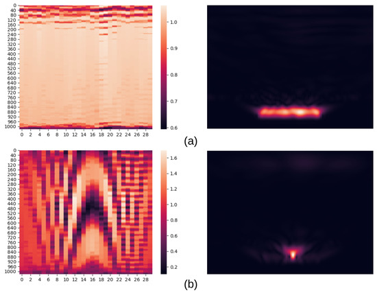
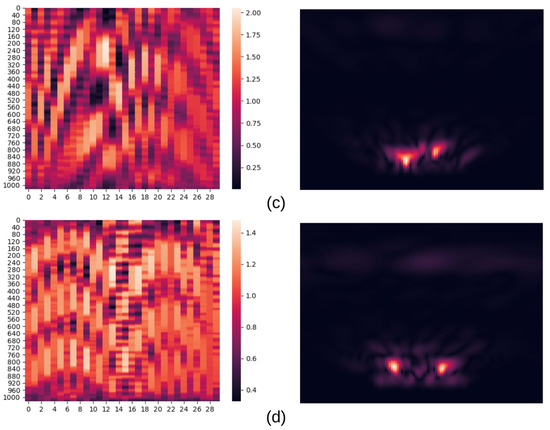
Figure 5.
Pairs of RealSAR-RAW (left) and RealSAR-IMG (right) examples. Example pair (a) represents an empty scene, (b) scene with an aluminium bottle, (c) scene with an aluminium and a glass bottle, while (d) contains all three bottles.
- Scaling: pixel colors in each reconstructed image represent different intensity. The pattern visible in reconstructed empty scene (Figure 5a) is actually crosstalk generated by the FMCW module and it is present in all measurements but is only noticeable in that image due to set scale. The scale was not fixed in order to prevent some objects (such as plastic bottle) to fade out from the reconstructed image.
- Angle of measurement: limited field of view due to finite GBSAR track size influences the representation of edge objects although virtual extension of azimuth axis is used in reconstruction algorithm to avoid compression of multiple images in the main field of view. In Figure 5b, aluminium bottle is set in the middle of the scene while in example Figure 5c it is set slightly to the right and more distant. It can be seen that the same object is differently represented in two reconstructed images.
- Difference in reflectance: in scenes where reflectance of one bottle is much higher than other bottle, after reconstruction process, one with lower reflectance can be hard to see. This problem can be spotted in reconstructed image of Figure 5d in which plastic bottle is not visible.
On the other hand, since input data in raw-based classification model is not preprocessed, the integrity of the data is preserved and, hence, such model has an advantage over image-based one.
Both variants of the RealSAR dataset were split into training, validation, and testing splits in the ratio of approximately 60:20:20. The splits consist of 204, 67, and 67 examples, respectively. A single class, in our setting, is any of the subsets of n different objects that can be present in the scene. Thus, in our case, there are 8 classes. The split was performed in a stratified fashion [43], meaning that the distribution of examples over different classes in each split corresponded to the distribution in the whole dataset. Since RealSAR-IMG was created by applying the Omega-K algorithm on examples in RealSAR-RAW, both variants contain the same examples. The training, validation, and testing splits, as well as any subset of the training set used in experiments, also contain the same examples in both RAW and IMG variants.
4. Deep Learning
4.1. End-to-End Learning vs. Feature Engineering
In classical machine learning, we usually need to transform our raw data to make it suitable as input to our machine learning model. We extract a set of features from each raw data point using classical algorithms or hand-crafted rules. The process of choosing an appropriate set of features with corresponding procedure for their extraction is called feature engineering [44].
With the advent of deep learning, approaches with fewer preprocessing steps have become more popular. Instead of manually transforming raw data into representations appropriate for the model, new model architectures were developed that were able to consume raw data [33]. Such models would implicitly learn their own optimal representations [34] of raw data, often outperforming model which learned on fixed, manually extracted features [45]. This paradigm is also referred to as end-to-end learning.
We designed our models and experiments to compare and contrast these two paradigms. The first approach is to use an existing image classification architecture ResNet18, which has been shown to be able to tackle a diverse set of computer vision problems [46,47]. This model is trained on RGB images reconstructed from radar data using Omega-K algorithm [39]. The second is an end-to-end learning approach, where the input is raw data collected with our GBSAR-Pi. The model architecture is based on ResNet18, with a few modifications to accommodate learning from raw data.
4.2. Multi-Task Learning and Multi-Label Classification
Our task consists of detecting the presence of multiple different objects in a scene. Instead of training a separate model for recognizing each individual object, we adopt the multi-task learning paradigm [48] and train only one model which recognizes all objects at once. The model consists of a single convolutional backbone which learns shared feature representations [49] that are then fed to multiple independent fully-connected binary classification output layers (heads). Each classification head is designated for classifying the presence of one of the objects which can appear in a scene. We calculate the binary cross-entropy loss for each head individually. The final loss which is optimized during training is the arithmetic mean of all individual binary cross entropy losses. The described formulation is also known as multi-label classification [50]. An alternative formulation would be to do multi-class classification. In multi-class classification, each possible subset of objects which can occur in a scene would be treated as a separate class. There would only be one head which would classify examples into only one of the classes. Although we do care that our model learns to recognize all possible object subsets well, we chose not to address the problem in this way because it does not scale. Namely, for n objects, there are different subsets. This means the number of outputs of a multi-class model grows exponentially with the number of objects that can appear in a scene. In contrast, in the multi-label formulation, there are only n outputs for n different objects.
4.3. Models
We train and evaluate multiple approaches for raw data and image-based classification. For image data, we test two popular efficient convolutional architectures for low-powered devices: MobileNetV3 [51] and ResNet18 [46], and compare their results. For raw radar data classification we consider two baseline approaches to compare against. The first is a single-layer fully connected classifier, while the second one uses an LSTM [52] network to process data before classifying it. We also apply the two convolutional architectures-MobileNetV3 and ResNet18-to classifiy raw radar data because of multiple reasons. Firstly, these networks have been shown to work well across a wide array of classification tasks. Secondly, the inductive biases and assumptions of convolutional neural networks regarding spatial locality [53] make sense for raw data as well. This is because raw radar data points are 2D matrices of values. The horizontal dimension corresponds to the lateral axis on which the radar moves as it records the scene (shown in Figure 5a). The values in the vertical dimension represent the signal after the mixer in FMCW system whose frequency correlates with the distance of objects. Finally, our main contribution in this regard is a modification to the ResNet18 network (RAW-RN18) when applied raw radar data, which prevents subsampling of the input matrix in the horizontal dimension.
Each of our image-based classification models takes a batch of RGB images with dimensions (496, 369, 3) as input. The pixels of RGB images are preprocessed by subtracting the mean and dividing by the standard deviation of pixel values, with statistics calculated on the train set. This is common in all computer vision approaches. For each image in the batch, the model outputs three numbers, each of which is then fed to the sigmoid activation function. The output of each sigmoid function is a posterior probability distribution , where . Each of the three distributions is the probability that the corresponding object (aluminium, glass, or plastic) is present in the scene. To summarize: .
Raw data classification models take a batch of 2D matrices of real numbers with dimensions (1024, 30, 1) as input. We preprocess raw data matrices in the same way that we do for images, with the raw data statistics also calculated on the train set. Raw data models produce the outputs in the same format as the image-based models. Figure 6 describes the machine learning setup for both input modalities.
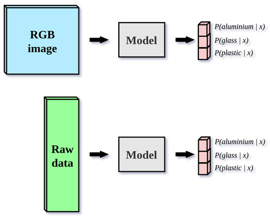
Figure 6.
The machine learning setup for all image and raw data models. For image-based classification, the dimensions of input images are (496, 369, 3). For raw data classification, the dimensions of the input matrix are (1024, 30, 1). All models produce three posterior probability distributions , where .
All models are trained in the multi-label classification fashion. For each of the three outputs, we separately calculate a binary cross-entropy loss: , where y is the ground truth label and is the predicted probability of the corresponding object. The total loss is calculated as the arithmetic mean of the three individual losses.
During training, we use random color jittering and horizontal flipping as data augmentation procedures. These are common ways of artificially increasing dataset size and improving model robustness in computer vision. To extend color jittering to raw data classification, we add Gaussian noise with variance to each element of the input matrix.
4.3.1. Baselines
We develop two baseline approaches for raw data classification. The first is a single-layer fully connected classification neural network. It flattens the input matrix of dimensions (1024, 30) into a vector of 30,720 elements. The vector is then fed to a fully-connected layer which produces the output vector with three elements. The network is shown in Figure 7. The second approach uses a single-layer bidirectional LSTM network for classification [54], which processes the inputs sequentially in the horizontal dimensions. It treats the input matrix with dimensions (1024, 30), as a sequence of 30 tokens with size 1024. Each 1024-dimensional input vector is embedded into a 256-dim representation by a learned embedding matrix [55], which is a standard way of transforming LSTM inputs. Because LSTM network is bidirectional, it aggregates the input sequence by processing it in both directions, using two separate unidirectional LSTM networks. The dimension of the hidden state is 256. The final hidden states of both directions are concatenated and then fed to a fully-connected classification layer. The network is shown in Figure 8.
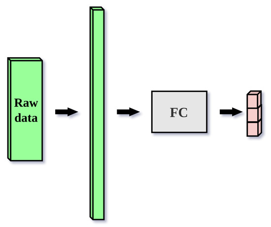
Figure 7.
Single-layer fully connected neural network classifier for raw data. The input matrix of dimensions (1024, 30, 1) is flattened into a vector of 30,720 elements. The vector is then fed to a fully connected classifier with the sigmoid activation function, which produces an output vector size 3 which represents three posterior probability distributions , where .
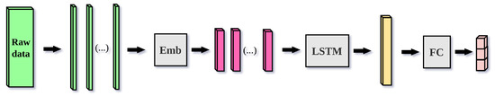
Figure 8.
Raw data classifier based on the long short term memory network. Since the LSTM is a sequential model, the input matrix with dimensions (1024, 30) is processed as a sequence of 30 vectors with size 1024. Each 1024-dimensional input vector is embedded into a 256-dim representation by a learned embedding layer (Emb). The dimension of the hidden state is 256. The bidirectional LSTM network aggregates the input sequence by processing it in two directions and concatenating the final hidden states for both directions. As with the fully connected classifier, the resulting vector is given to a fully connected classifier with the sigmoid activation function, which the three posterior probability distributions.
4.3.2. Computer Vision Models
For image-based classification, we employ two popular efficient convolutional neural network classification architectures: MobileNetV3 [51] and ResNet18 [46]. These lightweight, efficient, networks have been shown to work well across a wide array of classification tasks. We chose them because they are tailored to work on low-powered devices, such as Raspberry Pi, which we want to use to run model inference in real-time. Furthermore, the dataset which we developed is small so we opt for smaller models and forgo using larger classification architectures. We use both networks without any modifications for image and raw data classification.
Our main contribution came from analysing the ResNet18 architecture and devising an architectural modification to make the network more suitable for raw data classification. The ResNet18 network is composed of 17 convolutional layers and one fully-connected output layer. After the initial convolutional layer (conv1) which is followed by a max pooling layer, the remaining 16 convolutional layers are divided into 4 groups (conv2, conv3, conv4, conv5). Each group consists of 2 residual blocks, each of which consists of 2 convolutional layers. Residual blocks have skip (residual) connections which perform identity mapping and add the input of the residual block to the output of the two convolutional layers. In the vanilla ResNet18 architecture, the convolutional layers transform the input by gradually reducing the spatial dimensions and increasing the depth (number of feature maps). The spatial dimensions are halved in 5 places during the forward pass of the network, by using a stride of 2 in the following layers:
- The first convolutional layer (conv1);
- The max pooling layer before the first group of convolutional layers;
- The first convolutional layer of each of the remaining groups (conv3_1, conv4_1, conv5_1).
Figure 9 shows all of the ResNet18 layers and their groups, with the four convolutional layers which perform subsampling emphasized. Because the input tensor is halved in both spatial dimensions 5 times, output of the last convolutional layer is a tensor whose both spatial dimensions are 32 times smaller than that of the input. The depth of the tensor is 512. Global average pooling (GAP) is used to pool this tensor across the spatial dimensions into a vector of size 512. This shared representation is given as input to the fully-connected output layer which outputs a posterior probability for each object i.
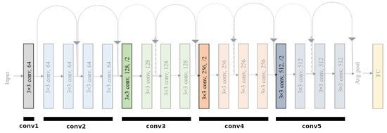
Figure 9.
All 17 convolutional layers and one fully-connected layer of the unmodified ResNet18 network. The convolutional layers are grouped into 5 groups: conv1, conv2, conv3, conv4, and conv5. There are four convolutional layers that downsample the input tensor by using a stride of 2. They are the first convolutional layers in groups conv1, conv3, conv4, and conv5. These layers are emphasized in the image. There is also a max pooling layer between groups conv1 and conv2, which also downsamples the image by using a stride of 2. Since the input image is downsampled five times, the resulting tensor which is output by the final convolutional layer is 32 times smaller in both spatial dimensions than the input image.
We considered the dimensionality of our input data: the vertical dimension is 1024, while the horizontal dimension is 30. Furthermore, while the two spatial dimensions of reconstructed images are similar (496 and 369), with an aspect ratio of 1.34, we can see this is not the case with raw radar data, where the horizontal dimension is much smaller than the vertical. In general, since we are focused on GBSAR with a limited aperture size, the horizontal dimension—which corresponds to the number of steps—will usually be low.
With that in mind, we see that the resulting tensor after the convolutional layers in ResNet18 is downsampled to have spatial dimensions (32, 1). Our modification changes the network so that it does not downsample the input data in the horizontal dimension at all. As we described, subsampling is performed in four of the convolutional layers and one max pooling layer of the network. In all cases, the subsampling is performed by using a stride of 2 in both spatial dimensions for the sliding window of either a convolutional or a max pooling layer. We change the horizontal stride of these downsampling layers from 2 to 1, while we keep the vertical stride unchanged. Figure 10 shows how the raw data input matrix is gradually subsampled in ResNet18 after the first convolutional layer (conv1), and each convolutional group (conv2, conv3, conv4, conv5), with and without our modification. The dimensions in the figure are not to scale since it would be impractical to display. Rather, it shows symbolically that without our modification, the horizontal dimension is subsampled from 30 to 1, while with the modification it remains 30.
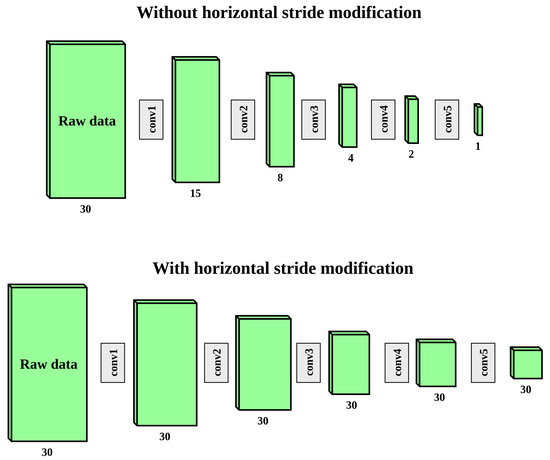
Figure 10.
The spatial dimensions of the input raw data matrix and subsequent subsampled intermediate representations after each group of convolutional layers. For groups conv1, conv3, conv4, and conv5, the subsampling is completed in the first convolutional layer of the group. For group conv2, the subsampling is completed in the max pooling layer immediately before the first convolutional layer of conv2. The first diagram show how, without any modification to the ResNet18 architecture, both the vertical and horizontal dimensions are halved five times. The vertical dimension is downsampled from 1024 to 32, while the horizontal dimension is downsampled from 30 to 1. The second diagram shows how only the vertical dimension is subsampled after our modification to the ResNet18 architecture, while the horizontal dimension remains constant. This is because our modification sets the horizontal stride of subsampling layers to 1. Note that the dimensions in the figure are not to scale due to impracticality of displaying very tall and narrow matrices.
This modification does not change the dimensionality of any kernels of the convolutional layers, so it does not add any parameters to the model. Thus, it does not prevent us from using any pretrained set of parameters of the original ResNet18 architecture. Even though the horizontal stride of the modified network is different, which can change the horizontal scale and appearance of features in deeper layers of the network, using existing ImageNet-pretrained weights is still a sensible initialization procedure. ImageNet pretraining has been shown to be consistently beneficial in a wide array of image classification tasks, some of which have different image dimensions, scales of objects appearing in the images, and even cover an entirely different domain of images than the ImageNet-1k dataset [56,57]. We empirically validate the contribution of pretraining for weight initialization in our experiments.
The modification results in the dimension of the tensor output by the last convolutional layer in the network being (32, 30), since the input is not subsampled in the horizontal dimension. The depth of that tensor remains 512, and the global average pooling layers aggregates this tensor across the spatial dimensions into a vector of size 512. Thus, the vector representation which is fed to the fully-connected output layer is of the same dimensionality as before the modification, the output layer also does not require any changes.
5. Experiments
5.1. Experiment Setup
To evaluate our models we perform experiments on the RealSAR dataset. We evaluate and compare two main approaches, each with a number of modifications regarding data augmentation procedures, weight initialization, the size of the training set and the classification architecture used. The first approach consists of models which work on reconstructed images. We train and evaluate them on the RealSAR-IMG dataset. In the second approach, we evaluate models which work with raw radar data. Experiments for the second approach are performed on the RealSAR-RAW dataset. All experiments were completed in a multi-label classification setting, where each label denotes the absence or presence of one of the three different objects that we detect. The training procedure minimized the mean of binary cross-entropy losses of all labels.
We chose all hyperparameters manually, by testing and comparing different combinations of values on the validation set. In all experiments for both models, we use the Adam optimizer, with a learning rate of , and the weight decay parameter set to .
Experiments on the full training set (156 examples) are performed over 30 epochs, with a batch size of 16, which results in 300 parameters updates. To ensure comparisons are fair, when training on subsets of the training set, the number of epochs is chosen, such that the total number of parameter updates stays the same.
To prevent our models from overfitting and increase robustness to noise, we use two stochastic data augmentation procedures during training: random horizontal flipping and color jittering. Since the radar moves laterally when recording a scene the raw recorded data are equivariant to changes in the lateral positions of objects in the scene. The Omega-K algorithm preserves the equivariance as well. Thus, for both the raw and the vision representation of any given scene, the horizontally flipped representation corresponds to rearranging the scene to be symmetric with respect to the middle of the lateral axis. Thus, the horizontal flip transformations does not change the semantics, i.e., the labels of that representation, and can be used as an augmentation procedure. Color jittering is used in computer vision to stochastically apply small photometric transformations on images. This artificially increases the dataset, since in every epoch, each image is transformed with different parameters, sampled randomly. One novelty we introduce is to extend this technique to raw data as well, by adding small Gaussian noise to each example. We validate this contribution empirically.
We trained both the raw and the image-based models with different modifications. To explore the contribution of transfer learning [34], we used three different weight initialization procedures: random initialization [58], initializing with ImageNet-1k pretrained weights, and initializing by pretraining on the LabSAR dataset. To test how the model improves as more data are collected, we performed experiments on 25%, 50%, 75%, and 100% of examples in the training set. The validation and test sets remained fixed throughout all experiments to ensure fair comparisons. Through these experiments we converged to the two best models: one based on raw radar data, and the other based on reconstructed images. We used these two models to performed further analyses.
To test whether combining models trained on different input modalities yields an increase in performance, we evaluated an ensemble model. The ensemble consists of the best RAW and the best IMG model. Its output vector is the mean of the output vectors of the two models.
5.2. Metrics
All of our models are trained in the multi-label classification setting. The model output P is a vector of n numbers, where n is the number of different objects which can appear in a scene. The element i of the output vector () is the probability given by the model that the corresponding object i is present in the scene. The probability of its absence is . Thus, the detection of each individual object can be seen as a separate binary classification problem.
In binary classification evaluation, we have a set of binary ground truth labels for all examples, and the corresponding model predictions, either as probabilities or as binary values (0 and 1). When the predictions are binary values, the pair consisting of the ground truth label and the prediction for any example in the dataset can be classified into one of four sets:
- True negative (TN): the object is not present, and the model predicts it correctly;
- False negative (FN): the object is present, but the model incorrectly predicts it is not;
- False positive (FP): the object is not present, but the model incorrectly predicts it is;
- True positive (TP): the object is present, and the model predicts it correctly.
Various metrics can be defined using the described quantities. Accuracy measures the percentage of correct predictions:
Precision (P) measures how many positive predictions were correct:
It decreases as the number of false positives increases. Recall (R) measures how many positive examples were captured:
It decreases as the number of false negatives increases. If we want a strict metric which will penalize both excessive false positives and false negatives, we can use the -score, which is the harmonic mean of precision and recall:
Since the output of the model is the probability of the positive class, we classify an example as a positive if the probability is higher than a certain threshold . Otherwise, we classify it as a negative. The natural threshold to choose is 0.5. However, the actual optimal threshold varies depending on the metric. For example, recall increases as the threshold decreases. The minimum threshold (0) will maximize recall (1.0), since it will capture all positive examples. A threshold that is higher than the highest prediction probability will minimize recall (0.0), since it will not capture any positive examples. Conversely, a higher threshold tends to result in higher precision, since only very certain predictions will be classified as positive.
To remove the variability of the choice of the threshold from model evaluation and comparison, the average precision (AP) metric is often used. It is calculated as the average over precision values for every possible recall value. To extend it to the multi-label setting (multiple binary classification problems), we use the mean average precision (mAP) which is the arithmetic mean of the AP values of all individual tasks.
Once the best model has been chosen according to mAP, in order to use it to make predictions, we have to find the optimal threshold parameter for each individual output. We want our model to perform well on all classes, i.e., all 8 possible subsets of objects that can appear in the scene. Thus, we choose a vector of thresholds such that it maximizes the macro- score on the validation set [59].
The macro- score is a multi-class extension of the score. It is calculated as the arithmetic mean over the -score of each class.
To calculate the -score of a given class in a multi-class setting, the results are reformulated as a binary classification problem. Class is treated as the positive class, while all other classes are grouped into one, negative, class. The multi-class confusion matrix is accordingly transformed into a binary confusion matrix. The quantities necessary for calculating the binary precision and recall values are then obtained as shown on Figure 11.
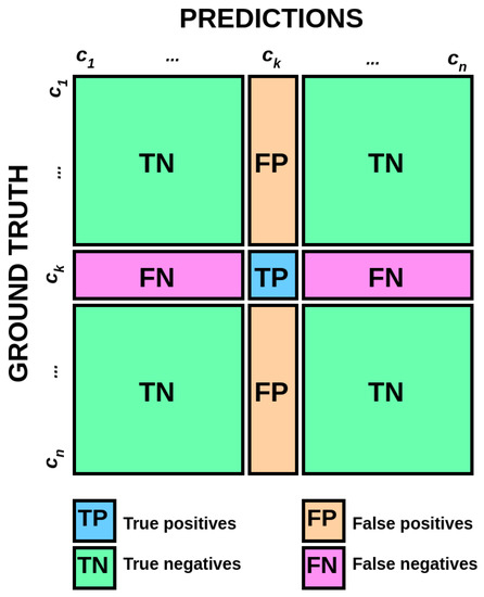
Figure 11.
The transformation of a multi-class confusion matrix into a binary confusion matrix for class . The macro- score is calculated as the arithmetic mean of scores of all classes [60].
5.3. Results
We consider two main approaches for GBSAR object classification, which correspond to the two possible input modalities: raw radar data (RAW) and reconstructed images (IMG). For raw data approaches, we compare five different classification architectures described in Section 4: the fully-connected baseline model (FC), the LSTM-based baseline model (LSTM), the ResNet18 (RN18) and MobileNetV3 (MNv3) convolutional architectures applied without any modifications, and, finally, our ResNet18 modified to handle raw radar data (RAW-RN18). For image-based approaches, we compare classifiers based on two convolutional architectures: ResNet18 and MobileNetV3.
Firstly, we validate the contribution of extending jittering as a data augmentation procedure to the raw input data modality. Table 2 shows the mAP results for all raw data approaches with and without jittering. For a given class, the AP metric averages the precision score over all possible recall scores, which correspond to different threshold values for classification. This makes our comparison of different variants of our approaches invariant to the threshold value. The mean AP score (mAP) is obtained by averaging the AP over all classes. It can be seen that jittering improves performance across the board. We also see that popular computer vision architectures ResNet18 and MobileNetV3 offer considerable improvements compared to the two baseline approaches, even when applied to raw data without any modification.
Table 2.
Comparison of performance of all raw data models with and without jittering. The metric used is mean average precision (mAP).
We compare all considered raw and image-based classification models, combined with different weight initialization procedures. The weight initialization procedures that we consider are the following: random initialization (random), pretraining on the LabSAR dataset (LabSAR), pretraining on the ImageNet-1k dataset (ImageNet), and pretraining on ImageNet-1k followed by LabSAR (ImageNet + LabSAR). Table 3 shows the mAP results for all combinations for the raw and image-based classification models. We see that ResNet18 and MobileNetV3 improve upon the baseline for both input modalities. However, for raw data, our modified ResNet18 (RAW-RN18), which ensures that the input tensor is not subsampled in the spatial dimension, significantly outperforms those models. As expected, we see that the vanilla, unmodified ResNet18 and MobileNetV3 architectures are more apt for image-based input, as they achieve significantly better results there compared to raw data. We also observe that out of the two convolutional architectures that we considered, the ResNet18 network consistently outperforms MobileNetV3 for this task. Finally, we can see that pretraining on ImageNet generally improves performance, while LabSAR pretraining is only beneficial in some cases, with a smaller impact. The knowledge learned from pretraining on LabSAR measurements with limited variance due to the controlled laboratory conditions in which they were captured proved not to transfer as significantly to the more complex RealSAR dataset.
Table 3.
Comparison of performance of all considered raw and image-based classification models in combination with all different weight initialization procedures on the validation set. The metric used is mean average precision (mAP).
Based on the results of these experiments, we converged to two main approaches for subsequent experiments. For raw data, we use our modified ResNet18 (RAW-RN18) model, while for image data we use the standard ResNet18. To observe how the size of the training dataset impacts performance, we train our models on subsets that contain 25%, 50%, and 75% of all training set examples. Thus, we perform training with all of the following combinations:
- Model type: IMG, RAW;
- Weight initialization: random, LabSAR pretrain, ImageNet-1k pretrain;
- Training set size: 1/4, 1/2, 3/4, Full;
The results on the validation set are displayed in Table 4. They show that models based on raw data experience a smaller drop in performance when trained on a smaller training set.
Table 4.
Comparison of performance of the two best model configurations for image and raw data classification. The chosen image model was an unmodified ResNet18 (RN18), while the chosen raw data model was a ResNet18 with our modification which prevents horizontal subsampling (RAW-RN18). We compare the two models across different weight initialization procedures and training set sizes on the validation set. The metric used is mean average precision (mAP).
We chose one RAW model and one IMG model with the best performance on the validation set to perform further analyses. The best IMG model was pretrained on ImageNet, while the best RAW model was pretrained first on ImageNet, then on LabSAR. Per-class AP scores on the test set for the two chosen models are displayed in Table 5. The mAP scores on the test set of both models are significantly lower than results on the validation set. This is expected since all results in Table 4 are chosen from the best epoch, as measured on the validation set. The validation set is used to choose the best hyperparameters for the model, as is standard practice in machine learning [43,61]. On the other hand, the test set results of chosen models are realistic mAP performance estimates. The RAW model has the higher AP score for classes aluminium and plastic, while the IMG model is slightly better for the glass bottles. The RAW model also has the higher mean AP score. This suggests that classification based on raw radar data, which circumvents lossy reconstruction steps, coupled with architectural modifications of neural networks can yield better performance than traditional computer vision approaches on reconstructed images. Figure 12 shows the average test mAP of the RAW and IMG pairs of models for each combination of the weight initialization scheme and training set size. We notice the general trend of increasing performance as the training set grows. The plots in the graph do not seem to be in a saturation regime, so additional data would be expected to increase the performance further. ImageNet pretraining is shown to be beneficial both in regards to the total performance and to the stability across different training set sizes.
Table 5.
Per-class AP performance of the best IMG and RAW models on the test set.
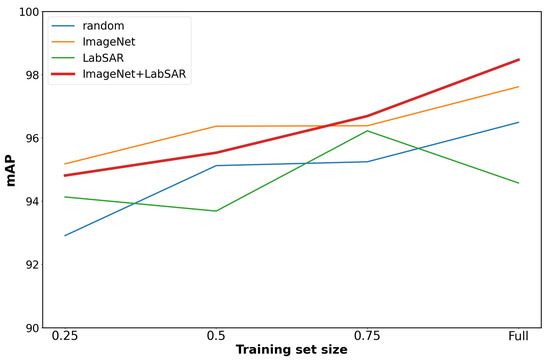
Figure 12.
Average test mAP of the RAW and IMG pair of models for each combination of weight initialization scheme and training set size.
To obtain a thorough evaluation of the performance of our two chosen models, we also test them in a multi-class setting. There are eight classes that cover all possible combinations of objects in the scene. In this way, we can get more insight into how the model behaves for objects when they appear individually in the scene versus how different groups of objects interact. This is especially interesting since the considered objects have varying reflectances and, thus, certain pairs of objects might be more difficult to discern among than others. We average the F1 score of each class to obtain the macro-F1 score. Although the comparison of different approaches in Table 4 was performed over all thresholds (mAP), for a multi-class comparison of the two chosen models, we need to choose concrete threshold parameters. For each of the two models, we find a threshold vector which maximizes the macro F1 score over all classes on the validation set. Table 6 shows the validation F1 score of each class, along with the macro F1 score, for both models. Once the threshold has been chosen using the validation set, we evaluate the models on the test set. The test set results are shown in Table 7. The RAW model outperforms the IMG model in all classes except for the glass–plastic combinations. The test set results also include the results of the ensemble model created by averaging the predictions of the two models.
Table 6.
Per-class F1 scores and the macro F1 score for the best threshold values on the validation set. E—Empty, A—Aluminium, P—Plastic, and G—Glass.
Table 7.
Per-class F1 scores and the macro F1 score of the two best models and their ensemble on the test set. Classes: E—Empty, A—Aluminium, P—Plastic, and G—Glass.
Out of the 67 test examples, the IMG model misclassifies 11 examples, while for the RAW model, the number of incorrect classifications is 8. This yields accuracy scores of 83.6% and 88.1%, respectively. Looking at the error sets, we found that all of the examples misclassified by the RAW model are also misclassified by the IMG model. In other words, there are no examples where the IMG model outperformed the RAW model. This explains why the ensemble model did not improve upon the performance of the single RAW model. The general idea of ensemble models is to aggregate predictions of different base estimators, each of which is more specialized in a certain sub-region of the input space than other estimators. In our case, the image-based model is not better than the raw model in any sub-region of the input space.
The confusion matrices of both models are shown in Figure 13a,b. The numbers of misclassified examples for different combinations of ground truth and prediction values are contained in elements off the diagonal.
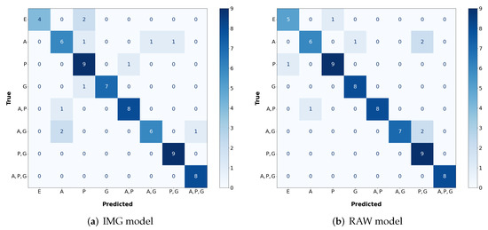
Figure 13.
Confusion matrices for the best IMG and RAW models. E—Empty, A—Aluminium, P—Plastic, and G—Glass.
6. Discussion
The main goal of this work was to compare two deep learning approaches for object classification on GBSAR data. Experimental results presented in the paper show that the model trained on raw data (RAW) consistently outperforms the image-based model (IMG), which uses the same data preprocessed with an image reconstruction algorithm. Specifically, out of 67 test examples, the IMG model misclassified 11, while the RAW model misclassified 8. The overlap of the two misclassification sets is peculiar. All 8 examples misclassified by the RAW model are also misclassified by the IMG model. This means there is no example in the test set where using the IMG model was beneficial compared to the RAW model. The three test examples where the IMG model made a mistake while the RAW model was correct (one of which is shown in Figure 14a indicate that reconstruction algorithms degrade the information in signals obtained by GBSAR due to approximations, as described in Section 2.2.
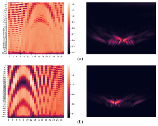
Figure 14.
RealSAR-RAW (left) and RealSAR-IMG (right) misclassified examples. Example (a) is misclassified by the IMG model while example (b) is misclassified by both RAW and IMG models. In (a) the recorded scene included a glass bottle, but IMG model classified it as plastic bottle. In (b) the recorded scene included an aluminium and a plastic bottle but both models classified it as scene with an aluminium bottle only.
Similar behavior is shown in Table 7: the F1 score is higher in the RAW model for every class except for the combination of glass and plastic (G, P). Half of the 8 examples incorrectly classified by the RAW model were predicted to be in the (G, P) class, as seen in the confusion matrix in Figure 13b. This significantly decreased the precision score, and, consequently, the F1 score, of the RAW model on that class. The table also shows that both models have difficulties classifying aluminium and combinations with aluminium. Aluminium has a much higher reflectance than glass and especially plastic. Consequently, it is hard for models to differentiate between scenes where the aluminium object appears alone versus ones where it appears together with another object of significantly lower reflectance. One such example is shown in Figure 14b, in which a scene containing both an aluminium and a plastic bottle is mistaken by both models for a scene containing only an aluminium bottle. The confusion matrices in Figure 13a,b also capture this phenomenon. Most of the misclassifications of both models are found in rows and columns that represent the aluminium class. The confusion matrices also highlight the difficulty of distinguishing an empty scene from one containing only a plastic bottle due to the very low reflectance of plastic.
In addition to reflectance and the aforementioned approximations, there is another factor impacting the results of the IMG model—the heatmap scale of reconstructed images. Total GBSAR signal intensities of scenes containing aluminium are much larger than signal intensities of empty scenes and scenes containing plastic bottles. Consequently, using a fixed scale in the visualization would result in objects fading out from reconstructed images due to their very high or very low intensity responses. By choosing not to set a fixed scale, we reduced the likelihood of such a scenario. However, this means that the resulting pixel intensities in reconstructed images are not absolute. For example, two pixels with equal color intensities in a scene with aluminium and an empty scene correspond to different raw signal intensities from which they were reconstructed. Hence, similar reconstructed images of two scenes with different objects can lead to misclassifications, such as the one presented in Figure 14a. RAW model classified that test example correctly as glass bottle, but IMG model mistook it with plastic one. In problems containing materials with less variance in terms of reflectance, the scale might be fixed.
Even though the comparisons between the two input modalities suggest the raw-data approach is superior, the usage of reconstructed images has certain advantages. Reconstructed images are more interpretable to humans, especially regarding the locations of the objects in the scene. It is extremely challenging for humans to discern objects and their locations in raw GBSAR data. Reconstructed images also allow for meaningful error analyses, making it easier to deduce why particular examples are misclassified. A valid paradigm might be to use raw data for the actual classification and only generate reconstructed images when we need to analyze specific examples or localize objects.
Regarding weight initialization, both models reached the highest classification accuracy when they were pretrained on the ImageNet dataset. ImageNet pretraining also decreased the variance of the results with respect to the size of the training set, as seen in the plot in Figure 12. Table 4 shows that the ImageNet-pretrained variant of the model based on reconstructed images achieved the highest mean average precision. In the case of the raw data model, the highest mAP was achieved by pretraining on both ImageNet and LabSAR datasets. This highlights the importance of pretraining and suggests that the RealSAR dataset might also be useful in future radar-related deep learning research.
7. Conclusions
The presented paper investigates the potential and benefits of processing raw GBSAR data in automated radar classification which can be particularly useful for industrial applications focused on monitoring and object detection in environments with limited visibility where this approach can save considerable resources and time. This differs from, and in this paper is contrasted with, the standard practice of applying classification algorithms on reconstructed images. The testing setup was developed around an FMCW based GBSAR system which was designed and constructed using low-cost components. The developed GBSAR was used in a series of measurements that were performed on several objects made of different materials with the final intention to realize a complete GBSAR radar system with embedded computer control capable of classifying these objects.
For classification purposes, a detailed analysis and comparison of two deep learning approaches to GBSAR object recognition was performed. The first approach was a more conventional SAR classification approach based on reconstructed GBSAR images, while in the second approach the classification was performed essentially on raw (unprocessed) data. Multiple different deep learning architectures for both approaches were trained, tested, and compared. These included two baselines based on fully-connected layers and LSTM networks, two standard convolutional neural network architectures-ResNet18 and MobileNetV3-popular in computer vision, and a modified variant of the ResNet18 network which makes it suitable for processing raw GBSAR data. The modification consists of preventing subsampling of the input in the horizontal dimension which is generally small due to the nature of GBSAR data. This modification is our main contribution regarding deep learning model design. The contribution was validated through experiments which showed that the best results on raw data are achieved by the modified version of ResNet18. Additionally, the practice of color jittering as a common data augmentation procedure in computer vision was extended to classification of raw GBSAR data and was shown to provide consistent, though small, improvements. Furthermore, it was shown that classification on raw data outperforms the classification based on reconstructed images. This was partially expected since the SAR image reconstruction algorithms necessarily introduce certain approximations, and with this negatively influence the integrity of the recorded data. In addition to better classification performance, raw data classification is inherently faster since it avoids the need for image reconstruction, and with this is more suitable for embedded computer implementation which opens possibilities for various application scenarios. On the other hand, it limits human visual confirmation and disables approaches in which radar images are combined with optical ones. However, keeping in mind that the primary focus is on applications in embedded systems, this is not a serious hindrance.
Even though this study has shown the applicability of this concept, it was tested using a relatively small dataset in order to focus on the comparison between approaches. Using larger datasets, more classes, and more general problem formulations could lead to more powerful and useful models. The other directions is to seek improvements in terms of more efficient networks and implementation in embedded computers with limited resources. With this in mind, for potential use in future research we generated and publicly released these datasets of raw GBSAR data and reconstructed radar images which we intend to update with time.
Author Contributions
Conceptualization, M.K., F.T., D.B. and M.B.; methodology, M.K., F.T., D.B. and M.B.; software, M.K. and F.T.; validation, M.K., F.T., D.B. and M.B.; formal analysis, M.K. and F.T.; investigation, M.K. and F.T.; resources, M.B.; data curation, M.K. and F.T.; writing—original draft preparation, M.K. and F.T.; writing—review and editing, D.B. and M.B.; visualization, M.K. and F.T.; supervision, D.B. and M.B.; project administration, M.B.; funding acquisition, M.B. All authors have read and agreed to the published version of the manuscript.
Funding
This work was supported in part by Croatian Science Foundation (HRZZ) under the project number IP-2019-04-1064.
Data Availability Statement
RealSAR datasets (RAW and IMG) used in this research are publicly available: https://data.mendeley.com/datasets/m458grc688/draft?a=ff342b09-dd03-4d09-a169-560af2f87773 (accessed on 1 November 2022).
Conflicts of Interest
The authors declare no conflict of interest.
Abbreviations
The following abbreviations are used in this manuscript:
| SAR | Synthetic Aperture Radar |
| GBSAR | Ground Based SAR |
| CNN | Convolutional Neural Network |
| FMCW | Frequency Modulated Continuous Wave |
| FFT | Fast Fourier Transform |
| IFFT | Inverse FFT |
| RPi | Microcomputer Raspberry Pi 4B |
| VCO | Voltage-Controlled Oscillator |
| SNR | Signal to Noise Ratio |
| AP | Average Precision |
| mAP | Mean Average Precision |
References
- Copernicus Space Component Mission Management Team. Sentinel High Level Operations Plan (HLOP). Available online: https://sentinels.copernicus.eu/documents/247904/685154/Sentinel+HLOP+-+Issue+3.1+-+16+Dec+2021.pdf (accessed on 23 July 2022).
- Liu, B.; He, K.; Han, M.; Hu, X.; Ma, G.; Wu, M. Application of UAV and GB-SAR in Mechanism Research and Monitoring of Zhonghaicun Landslide in Southwest China. Remote Sens. 2021, 13, 1653. [Google Scholar] [CrossRef]
- Izumi, Y.; Zou, L.; Kikuta, K.; Sato, M. Anomalous Atmospheric Phase Screen Compensation in Ground-Based SAR over Mountainous Area. In Proceedings of the IGARSS 2019—2019 IEEE International Geoscience and Remote Sensing Symposium, Yokohama, Japan, 28 July–2 August 2019; pp. 2030–2033. [Google Scholar] [CrossRef]
- Chet, K.V.; Siong, L.C.; Hsin, W.H.H.; Wei, L.L.; Guey, C.W.; Yam, C.M.; Sze, L.T.; Kit, C.Y. Ku-band ground-based SAR experiments for surface deformation monitoring. In Proceedings of the 2015 IEEE 5th Asia-Pacific Conference on Synthetic Aperture Radar (APSAR), Singapore, 1–4 September 2015; pp. 641–644. [Google Scholar] [CrossRef]
- Ma, Z.; Mei, G.; Prezioso, E.; Zhang, Z.; Xu, N. A deep learning approach using graph convolutional networks for slope deformation prediction based on time-series displacement data. Neural Comput. Appl. 2021, 33, 14441–14457. [Google Scholar] [CrossRef]
- Tarchi, D.; Antonello, G.; Casagli, N.; Farina, P.; Fortuny-Guasch, J.; Guerri, L.; Leva, D. On the Use of Ground-Based SAR Interferometry for Slope Failure Early Warning: The Cortenova Rock Slide (Italy). In Landslides: Risk Analysis and Sustainable Disaster Management; Sassa, K., Fukuoka, H., Wang, F., Wang, G., Eds.; Springer: Berlin/Heidelberg, Germany, 2005; pp. 337–342. [Google Scholar] [CrossRef]
- Martinez-Vazquez, A.; Fortuny-Guasch, J. A GB-SAR Processor for Snow Avalanche Identification. IEEE Trans. Geosci. Remote Sens. 2008, 46, 3948–3956. [Google Scholar] [CrossRef]
- Miccinesi, L.; Consumi, T.; Beni, A.; Pieraccini, M. W-band MIMO GB-SAR for Bridge Testing/Monitoring. Electronics 2021, 10, 2261. [Google Scholar] [CrossRef]
- Qiu, Z.; Jiao, M.; Jiang, T.; Zhou, L. Dam Structure Deformation Monitoring by GB-InSAR Approach. IEEE Access 2020, 8, 123287–123296. [Google Scholar] [CrossRef]
- Du, S.; Feng, G.; Wang, J.; Feng, S.; Malekian, R.; Li, Z. A New Machine-Learning Prediction Model for Slope Deformation of an Open-Pit Mine: An Evaluation of Field Data. Energies 2019, 12, 1288. [Google Scholar] [CrossRef]
- Kang, M.K.; Kim, K.E.; Cho, S.J.; Lee, H.; Lee, J.H. Wishart supervised classification results of C-band polarimetric GB-SAR image data. In Proceedings of the 2011 IEEE International Geoscience and Remote Sensing Symposium, Vancouver, BC, Canada, 24–29 July 2011; pp. 459–462. [Google Scholar] [CrossRef]
- Feng, S.; Ji, K.; Zhang, L.; Ma, X.; Kuang, G. SAR Target Classification Based on Integration of ASC Parts Model and Deep Learning Algorithm. IEEE J. Sel. Top. Appl. Earth Obs. Remote Sens. 2021, 14, 10213–10225. [Google Scholar] [CrossRef]
- Liu, H.; Li, S. Decision fusion of sparse representation and support vector machine for SAR image target recognition. Neurocomputing 2013, 113, 97–104. [Google Scholar] [CrossRef]
- Huang, Z.; Pan, Z.; Lei, B. Transfer Learning with Deep Convolutional Neural Network for SAR Target Classification with Limited Labeled Data. Remote Sens. 2017, 9, 907. [Google Scholar] [CrossRef]
- Chen, S.; Wang, H.; Xu, F.; Jin, Y.Q. Target Classification Using the Deep Convolutional Networks for SAR Images. IEEE Trans. Geosci. Remote Sens. 2016, 54, 4806–4817. [Google Scholar] [CrossRef]
- Liu, J.; Xing, M.; Yu, H.; Sun, G. EFTL: Complex Convolutional Networks With Electromagnetic Feature Transfer Learning for SAR Target Recognition. IEEE Trans. Geosci. Remote Sens. 2022, 60, 1–11. [Google Scholar] [CrossRef]
- Zhang, J.; Xing, M.; Xie, Y. FEC: A Feature Fusion Framework for SAR Target Recognition Based on Electromagnetic Scattering Features and Deep CNN Features. IEEE Trans. Geosci. Remote Sens. 2021, 59, 2174–2187. [Google Scholar] [CrossRef]
- Pei, J.; Huang, Y.; Huo, W.; Zhang, Y.; Yang, J.; Yeo, T.S. SAR Automatic Target Recognition Based on Multiview Deep Learning Framework. IEEE Trans. Geosci. Remote Sens. 2018, 56, 2196–2210. [Google Scholar] [CrossRef]
- Wagner, S.A. SAR ATR by a combination of convolutional neural network and support vector machines. IEEE Trans. Aerosp. Electron. Syst. 2016, 52, 2861–2872. [Google Scholar] [CrossRef]
- Li, J.; Qu, C.; Peng, S.; Jiang, Y. Ship Detection in SAR images Based on Generative Adversarial Network and Online Hard Examples Mining. Dianzi Yu Xinxi Xuebao/J. Electron. Inf. Technol. 2019, 41, 143–149. [Google Scholar] [CrossRef]
- Li, J.; Qu, C.; Peng, S.; Deng, B. Ship detection in SAR images based on convolutional neural network. Xi Tong Gong Cheng Yu Dian Zi Ji Shu/Syst. Eng. Electron. 2018, 40, 1953–1959. [Google Scholar] [CrossRef]
- Zhang, T.; Zhang, X. High-Speed Ship Detection in SAR Images Based on a Grid Convolutional Neural Network. Remote Sens. 2019, 11, 1206. [Google Scholar] [CrossRef]
- Li, J.; Qu, C.; Shao, J. Ship detection in SAR images based on an improved faster R-CNN. In Proceedings of the 2017 SAR in Big Data Era: Models, Methods and Applications (BIGSARDATA), Beijing, China, 13–14 November 2017; pp. 1–6. [Google Scholar] [CrossRef]
- Xia, R.; Chen, J.; Huang, Z.; Wan, H.; Wu, B.; Sun, L.; Yao, B.; Xiang, H.; Xing, M. CRTransSar: A Visual Transformer Based on Contextual Joint Representation Learning for SAR Ship Detection. Remote Sens. 2022, 14, 1488. [Google Scholar] [CrossRef]
- Koyama, C.N.; Sato, M. Detection and classfication of subsurface objects by polarimetric radar imaging. In Proceedings of the 2015 IEEE Radar Conference, Johannesburg, South Africa, 27–30 October 2015; pp. 440–445. [Google Scholar] [CrossRef]
- Yigit, E.; Demirci, S.; Unal, A.; Ozdemir, C.; Vertiy, A. Millimeter-wave Ground-based Synthetic Aperture Radar Imaging for Foreign Object Debris Detection: Experimental Studies at Short Ranges. J. Infrared Millim. Terahertz Waves 2012, 33, 1227–1238. [Google Scholar] [CrossRef]
- Zhang, T.; Zhang, X.; Ke, X.; Zhan, X.; Shi, J.; Wei, S.; Pan, D.; Li, J.; Su, H.; Zhou, Y.; et al. LS-SSDD-v1.0: A Deep Learning Dataset Dedicated to Small Ship Detection from Large-Scale Sentinel-1 SAR Images. Remote. Sens. 2020, 12, 2997. [Google Scholar] [CrossRef]
- Zhang, T.; Zhang, X. A Dual-Polarization Information Guided Network for SAR Ship Classification. arXiv 2022, arXiv:2207.04639. [Google Scholar] [CrossRef]
- Zhang, T.; Zhang, X. A polarization fusion network with geometric feature embedding for SAR ship classification. Pattern Recognit. 2022, 123, 108365. [Google Scholar] [CrossRef]
- Zhang, T.; Zhang, X.; Liu, C.; Shi, J.; Wei, S.; Ahmad, I.; Zhan, X.; Zhou, Y.; Pan, D.; Li, J.; et al. Balance learning for ship detection from synthetic aperture radar remote sensing imagery. ISPRS J. Photogramm. Remote Sens. 2021, 182, 190–207. [Google Scholar] [CrossRef]
- Zhang, T.; Zhang, X. A Mask Attention Interaction and Scale Enhancement Network for SAR Ship Instance Segmentation. arXiv 2022, arXiv:2207.03912. [Google Scholar] [CrossRef]
- Zhang, T.; Zhang, X. HTC+ for SAR Ship Instance Segmentation. Remote Sens. 2022, 14, 2395. [Google Scholar] [CrossRef]
- Schmidhuber, J. Deep learning in neural networks: An overview. Neural Netw. 2015, 61, 85–117. [Google Scholar] [CrossRef]
- Bengio, Y. Deep Learning of Representations: Looking Forward. In SLSP 2013: Statistical Language and Speech Processing, Proceedings of the First International Conference, SLSP 2013, Tarragona, Spain, 29–31 July 2013; Lecture Notes in Computer, Science; Dediu, A., Martín-Vide, C., Mitkov, R., Truthe, B., Eds.; Springer: Berlin/Heidelberg, Germany, 2013; Volume 7978, pp. 1–37. [Google Scholar] [CrossRef]
- Amézaga, A.; López-Martínez, C.; Jové, R. A Multi-Frequency FMCW GBSAR: System Description and First Results. In Proceedings of the 2021 IEEE International Geoscience and Remote Sensing Symposium IGARSS, Brussels, Belgium, 11–16 July 2021; pp. 1943–1946. [Google Scholar] [CrossRef]
- Jankiraman, M. FMCW Radar Design; Artech House: London, UK, 2018. [Google Scholar]
- Guo, S.; Dong, X. Modified Omega-K algorithm for ground-based FMCW SAR imaging. In Proceedings of the 2016 IEEE 13th International Conference on Signal Processing (ICSP), Chengdu, China, 6–10 November 2016; pp. 1647–1650. [Google Scholar] [CrossRef]
- Cruz, H.; Véstias, M.; Monteiro, J.; Neto, H.; Duarte, R.P. A Review of Synthetic-Aperture Radar Image Formation Algorithms and Implementations: A Computational Perspective. Remote Sens. 2022, 14, 1258. [Google Scholar] [CrossRef]
- Giroux, V.; Cantalloube, H.; Daout, F. An Omega-K algorithm for SAR bistatic systems. In Proceedings of the 2005 IEEE International Geoscience and Remote Sensing Symposium, IGARSS’05, Seoul, Korea, 29 July 2005; IEEE: New York, NY, USA, 2005; Volume 2, pp. 1060–1063. [Google Scholar]
- Hamasaki, T.; Ferro-Famil, L.; Pottier, E.; Sato, M. Applications of polarimetric interferometric ground-based SAR (GB-SAR) system to environment monitoring and disaster prevention. In Proceedings of the European Radar Conference 2005—EURAD 2005, Paris, France, 3–4 October 2005; pp. 29–32. [Google Scholar] [CrossRef]
- Innosent. Radar Sensor IVS-362. Available online: https://www.innosent.de/en/radarsensoren/ivs-series/ivs-362/ (accessed on 19 July 2022).
- RSHub FER. Omega-K Algorithm in Python. Available online: https://github.com/filt27/OmegaK/blob/main/OmegaK.py (accessed on 24 July 2022).
- Ojala, M.; Garriga, G.C. Permutation Tests for Studying Classifier Performance. J. Mach. Learn. Res. 2010, 11, 1833–1863. [Google Scholar] [CrossRef]
- Zheng, A.; Casari, A. Feature Engineering for Machine Learning: Principles and Techniques for Data Scientists, 1st ed.; O’Reilly Media, Inc.: Sebastopol, CA, USA, 2018. [Google Scholar]
- Collobert, R.; Weston, J.; Bottou, L.; Karlen, M.; Kavukcuoglu, K.; Kuksa, P.P. Natural Language Processing (Almost) from Scratch. J. Mach. Learn. Res. 2011, 12, 2493–2537. [Google Scholar] [CrossRef]
- He, K.; Zhang, X.; Ren, S.; Sun, J. Deep Residual Learning for Image Recognition. In Proceedings of the 2016 IEEE Conference on Computer Vision and Pattern Recognition, CVPR 2016, Las Vegas, NV, USA, 27–30 June 2016; IEEE Computer Society: New York, NY, USA, 2016; pp. 770–778. [Google Scholar] [CrossRef]
- He, K.; Zhang, X.; Ren, S.; Sun, J. Identity Mappings in Deep Residual Networks. In ECCV 2016: Computer Vision—ECCV 2016, Proceedings of the 14th European Conference, Amsterdam, The Netherlands, 11–14 October 2016; Leibe, B., Matas, J., Sebe, N., Welling, M., Eds.; Part IV; Lecture Notes in Computer Science; Springer: Berlin/Heidelberg, Germany, 2016; Volume 9908, pp. 630–645. [Google Scholar] [CrossRef]
- Collobert, R.; Weston, J. A unified architecture for natural language processing: Deep neural networks with multitask learning. In Machine Learning, Proceedings of the Twenty-Fifth International Conference (ICML 2008), Helsinki, Finland, 5–9 June 2008; Cohen, W.W., McCallum, A., Roweis, S.T., Eds.; ACM International Conference Proceeding Series; ACM: Rochester, NY, USA, 2008; Volume 307, pp. 160–167. [Google Scholar] [CrossRef]
- Bengio, Y.; Courville, A.C.; Vincent, P. Representation Learning: A Review and New Perspectives. IEEE Trans. Pattern Anal. Mach. Intell. 2013, 35, 1798–1828. [Google Scholar] [CrossRef]
- Boutell, M.R.; Luo, J.; Shen, X.; Brown, C.M. Learning multi-label scene classification. Pattern Recognit. 2004, 37, 1757–1771. [Google Scholar] [CrossRef]
- Howard, A.; Pang, R.; Adam, H.; Le, Q.V.; Sandler, M.; Chen, B.; Wang, W.; Chen, L.; Tan, M.; Chu, G.; et al. Searching for MobileNetV3. In Proceedings of the 2019 IEEE/CVF International Conference on Computer Vision, ICCV 2019, Seoul, Korea, 27 October–2 November 2019; IEEE: New York, NY, USA, 2019; pp. 1314–1324. [Google Scholar] [CrossRef]
- Hochreiter, S.; Schmidhuber, J. Long Short-Term Memory. Neural Comput. 1997, 9, 1735–1780. [Google Scholar] [CrossRef]
- Krizhevsky, A.; Sutskever, I.; Hinton, G.E. ImageNet classification with deep convolutional neural networks. Commun. ACM 2017, 60, 84–90. [Google Scholar] [CrossRef]
- Yildirim, Ö. A novel wavelet sequence based on deep bidirectional LSTM network model for ECG signal classification. Comput. Biol. Med. 2018, 96, 189–202. [Google Scholar] [CrossRef] [PubMed]
- Mikolov, T.; Sutskever, I.; Chen, K.; Corrado, G.S.; Dean, J. Distributed Representations of Words and Phrases and their Compositionality. In Advances in Neural Information Processing Systems 26, Proceedings of the 27th Annual Conference on Neural Information Processing Systems 2013, Lake Tahoe, NV, USA, 5–8 December 2013; Burges, C.J.C., Bottou, L., Ghahramani, Z., Weinberger, K.Q., Eds.; Curran Associates, Inc.: Red Hook, NY, USA, 2013; pp. 3111–3119. [Google Scholar]
- Studer, L.; Alberti, M.; Pondenkandath, V.; Goktepe, P.; Kolonko, T.; Fischer, A.; Liwicki, M.; Ingold, R. A Comprehensive Study of ImageNet Pre-Training for Historical Document Image Analysis. In Proceedings of the 2019 International Conference on Document Analysis and Recognition, ICDAR 2019, Sydney, Australia, 20–25 September 2019; IEEE: New York, NY, USA, 2019; pp. 720–725. [Google Scholar] [CrossRef]
- Cherti, M.; Jitsev, J. Effect of pre-training scale on intra- and inter-domain, full and few-shot transfer learning for natural and X-ray chest images. In Proceedings of the International Joint Conference on Neural Networks, IJCNN 2022, Padua, Italy, 18–23 July 2022; IEEE: New York, NY, USA, 2022; pp. 1–9. [Google Scholar] [CrossRef]
- Glorot, X.; Bengio, Y. Understanding the difficulty of training deep feedforward neural networks. In Proceedings of the Thirteenth International Conference on Artificial Intelligence and Statistics, AISTATS 2010, Chia Laguna Resort, Sardinia, Italy, 13–15 May 2010; Volume 9, pp. 249–256. [Google Scholar]
- Fujino, A.; Isozaki, H.; Suzuki, J. Multi-label Text Categorization with Model Combination based on F1-score Maximization. In Proceedings of the Third International Joint Conference on Natural Language Processing, IJCNLP 2008, Hyderabad, India, 7–12 January 2008; The Association for Computer Linguistics: Stroudsburg, PA, USA, 2008; pp. 823–828. [Google Scholar]
- Krüger, F. Activity, Context, and Plan Recognition with Computational Causal Behaviour Models. Ph.D. Thesis, University of Rostock, Rostock, Germany, 2016. [Google Scholar]
- Yao, Y.; Rosasco, L.; Caponnetto, A. On Early Stopping in Gradient Descent Learning. Constr. Approx. 2007, 26, 289–315. [Google Scholar] [CrossRef]
Publisher’s Note: MDPI stays neutral with regard to jurisdictional claims in published maps and institutional affiliations. |
© 2022 by the authors. Licensee MDPI, Basel, Switzerland. This article is an open access article distributed under the terms and conditions of the Creative Commons Attribution (CC BY) license (https://creativecommons.org/licenses/by/4.0/).