Abstract
The Mediterranean ecosystem exhibits a particular geology and climate, which is characterized by mild, rainy winters and long, very hot summers with low precipitation; it has led to the emergence of resilient plant species. Such habitats contain a preponderance of shrubs, and collectively harbor 10% of the Earth’s species, thus containing some of the most unique shrubby formations protecting against environmental natural degradation. Due to shrub species diversity, initial phases of forestland, heterogenous grasses, bare ground and stones, the monitoring of such areas is difficult. For this reason, the aim of this paper is to assess semi-automatic classifications of the shrubby formations based on multispectral Sentinel-2 and visible and near infrared (VINR) AISA-EAGLE II hyperspectral airborne images with a support of Canopy High Model (CHM) as a three-dimensional information and field-verified patterns, based on Match-T/DSM and aerial photos. Support Vector Machine (SVM) and Random Forest (RF) classifiers have been tested on a few scenarios featuring different combinations of spectral and Minimum Noise Fraction (MNF) transformed bands and vegetation indices. Referring to the results, the average overall accuracy for the SVM and AISA images (all tested data sets) was 78.23%, and for the RF: 79.85%. In the case of Sentinel-2, the SVM classifier obtained an average value of 83.63%, while RF: 85.32%; however, in the case of the shrubland, we would like to recommend the RF classifier, because the highest mean value of F1-score achieved was 91.86% (SVM offered few-percent-point worse results), and the required training time was quicker than SVM. Commonly available Sentinel-2 data offered higher accuracies for shrubland monitoring than did the airborne VNIR data.
1. Introduction
Shrubland (alternative terms: scrubs, scrubland, shrubland, shrubby formation, chaparral) covers all kind of woody formations dominated by shrubs (perennial woody plants not exceeding 5–8 m height) with herbs, grasses and geophytes [1]. In particular regions, it may be a stable type of vegetation or a transitional stage in the ecological succession after a fire, deforestation or agricultural wastelands. The world’s main areas of shrubland occur in the Mediterranean climate (wet, mild, long winters and hot, dry summers) [2]. Natural shrublands have the lowest water consumption and better resist climate aridification compared to other stands, e.g., trees, which cannot survive such harsh conditions [3]. Shrubs facilitate rainwater infiltration, protect soil from erosion and optimize a carbon exchange, thereby limiting its emission into the atmosphere [4,5]. Disruption of this vegetation causes an increase in soil surface temperature, plant water stress and erosion effect on runoff and sediment yield [6]. The importance of the occurrence of shrubs in the Mediterranean environment is also described by Torre et al. [7], analyzing airborne lidar scanning (ALS) data, vegetation profiles for a decade period for selected study plots in Barcelona’s Natural Parks, (Catalonia, NE Spain) where the relationship of shrubs vegetation cover and the occurrence of small mammals was studied. These play a key role in the sustainability of Mediterranean forests; therefore, monitoring scrubs plots is important from a management perspective under current conditions of global change. In Catalonia, as in many Mediterranean countries, the amount of precipitation is insufficient to maintain the dense vegetation cover that helps prevent a loss of habitat biodiversity [8]. Shrublands cover approximately 14% of Catalonia, being one of the main vegetated covers [1], and monitoring of shrub spatial distribution allows biomass monitoring, which provides some of the key input data for fire risk estimation; biomass and its parameters are frequently discussed issues in the case of remote sensing shrub analysis. Calvão and Palmeirim [9] identified Mediterranean scrubs (authors use this term) located in SE Portugal on Landsat images, which allowed for the calculation of a Normalized Difference Vegetation Index (NDVI); least-squares linear regression model verified by field-acquired data from experimental sites describing leaf, woody and litter biomass, canopy cover and Leaf Area Index (LAI) allowed for the capture of phenological spectral changes of the Cistus spp. and the evergreen sclerophyllous scrubs, and correlations between NDVI, canopy cover and fresh biomass was shown to oscillate around r=−0.53, p < 0.02 [9]. In the following paper, Calvão and Palmeirim [10] also confirmed monitoring capabilities of long-term Mediterranean vegetation changes based on 12 Landsat-derived vegetation indices (VIs) characterizing the state of plants (including soil properties) and biophysical parameters (biomass and leaf area indices, canopy height and cover), which allowed for the development of regression models; normalized difference VIs correlated well with canopy-oriented variables (r = 0.83–0.86) and worse correlated with leaf-related variables (r = 0.59). The analyses confirmed that the most useful indices were Ratio Vegetation Index = Simple Ratio (RVI) and NDVI, and Renormalized Difference Vegetation Index (RDVI), Modified Simple Ratio (MSR), Leaf Area Index (LAI) and Landsat bands scored worse, non-significant correlation values (<0.58). Similar results were achieved for High-Arctic shrubs [11,12] and for alpine meadow plants [13,14,15]. Sentinel-2 images were also successfully used to identify multi-temporal shrubland areas in Inner Mongolia, China [16] and in deforested equatorial areas of Gabon [17]. In the first case, the authors [16] described the importance of the phenological factor in identifying shrubs. For this purpose, the authors used the gaussian process regression (GPR, determining similarity between samples) and random forest regression (RFR, indicating a degree of mean square error (MSE) reduction of feature variables), which were the vegetation indices presented below. The conducted analyses confirmed that early spring (early April), summer (late June-mid-July) and late October are optimal periods for shrubs analysis (in our case, various growing periods were not analyzed, as we had access to the data acquired during a single AISA flight campaign, and the Sentinel-2 image was selected in accordance with the airborne data). Gan et al. [16] also selected relevant vegetation indices for this type of analysis, which were NDTI (Normalized Difference Tillage Index), GNDVI (Green Normalized Difference Vegetation Index), NDVI, NDSVI (Normalized Difference Senescent Vegetation Index), EVI2 (two-band Enhanced Vegetation Index), MSAVI, NDPI (Normalized Difference Phenology Index), NDGI (Normalized Difference Greenness Index) and NDMI (Normalized Difference Moisture Index). As the outcome, Caragana shrubs were identified with the best overall accuracy, achieving 91.7%, and RMSE achieved 5.0–5.5% (validation–test patterns). A significant role of increasing the results were found with the NDTI and NDGI indices [16]. In the case of Gabonese research, authors tested an increase of DEM and NDVI on the accuracy of Sentinel-2 image classification carried out with the Random Forest (RF) algorithm. The results confirmed that non-forest communities achieved 76.4–96.1% (Producer Accuracy), and the DEM increased outcomes by six percent points compared to the set which contained only the NDVI index [17].
Estimated shrub biomass in formerly burned areas was estimated in many countries, e.g., in Portugal [18]; the authors used 10-m-Sentinel-2 NDVI to create a raster mask for identifying burnt areas, and using Minimum Distance Classifier and B2, B3, B4 and B8 bands (VIS–NIR), identified forested and shrubland areas with an overall accuracy (OA) oscillating around 80% (Cohen’s K coefficient k = 0.75) [18]. Bulk density for shrubs has also been studied to estimate carbon sequestration, which could assist in predicting the potential fire risk for the Iberian Peninsula [19]. Vega et al. [20], based on the field surveys and biomass measurements, raised the shrubs communities biomass modelling in Northern Spain and developed models for standing fuel loads by size and condition. Biomass estimation plays a particularly important role in determining the fuel source for shrublands fires and greenhouse gas emission. Sentinel-2, TanDEM-X and airborne LiDAR data and Random Forest with an option of automatic feature selection allowed for the mapping of shrublands with 83.1% overall accuracy (balanced accuracy scored 0.82) [21], and the achieved results allowed for the prediction of landscape biomass (Spearman rank correlation achieved 0.80–0.84, and normalized RMSE <16%). The authors [21] also highlighted an integration of vegetation type mapping towards biomass, water and carbon management modelling based on remote sensing data. More complicated spatial systems, in the form of 24 classes of homogeneous scrub communities of Western Australia were identified on multitemporal Sentinel-2 images [22]. The authors tested a few scenarios oriented on growing seasons, data compression methods and used input data, and the best results were achieved for Sentinel-2 spring and autumn spectral bands and tasseled cap transformed data classifying by the SVM (average value oscillated between 72–74%), worse results were noted for Nearest Neighbour (NN)–72%, RF–65% and Classification Trees (CT)–50% [22]. Similar research was conducted in Portugal in frame of a M.Sc. thesis [23]; Sequeira and his supervisors used multitemporal Sentinel-2 data, which classified 31 classes: 14 crop and 17 land cover types by RF with an overall accuracy of 76%, and the shrubland scored 70% (user accuracy, UA), 63% (producer accuracy, PA) and achieved an F1-score of 67%. The researcher also confirmed that shrubland, grasslands, bare soil and sparse vegetation were often mixed, because spectral signals (mixels) consisted of green, dry vegetation and different fractions of soil and shadow [23].
Different classifiers were used for land cover and plant community identification; based on 144 bands of hyperspectral images (in the spectral range of 380–1050 nm), Khodadadzadeh et al. [24] compared different classifiers, e.g., SVM and CNN (Convolutional Neural Network) for vegetation mapping [25,26]. The best results were achieved for: Joint Sparse Representation (86.86% of overall accuracy), while CNN and SVM scored 86% [26]. Often SVM, RF and other machine learning methods are successfully implemented to identify plant communities, as well as species achieving comparable level of overall accuracies (85–92%) [27,28,29,30]. In the papers, the authors used data spectral bands with different remote sensing indices, e.g., Enhanced Vegetation Index (EVI) or NDVI [31,32] as inputs, which made it easier to distinguish types of communities [33,34] and species [35]. In addition, Airborne Laser Scanner (ALS) data were also used, which allowed for the characterization of the multi-story spread of land cover and for the classification of the different species [36]. Integration of PlanetScope images and LiDAR point clouds gave good results for the land cover classification [37]. The authors, based on random trees method, mapped transitional shrubs with herbaceous communities areas with an accuracy of 97.19% (UA) and 87.82% (PA) [37]. The Random Forest classifier offers faster data processing time than the SVM classifier while offering comparable average accuracies to the SVMs [38]. Application of Sentinel-2 data, specifically the red-edge band for detection and mapping of mountain shrublands, was also highlighted by Bayle et al. [39], who compared the effectiveness of Normalized Anthocyanin Reflectance Index (NARI, which is a normalization of the ARI = 1/R550 – 1/R700 index [40]) to NDVI for shrubby formation mapping. NARI, indicating anthocyanin content in the canopy, achieved 0.92, and NDVI 0.58 (measuring the Area Under the Curve, AUC), which, after verification of the model, allowed for the evaluation of the final shrub cover map with a Kappa coefficient equal to 0.67, confirmed that the Sentinel-2 red-edge band delivers extended opportunities to detect shrubby formations.
Due to climate changes manifested by an increase in the frequency of high air temperatures and a decrease in the amount of rainfall, the Mediterranean ecosystem is exposed to water stress, which leads to a risk of vegetation, soil and rhizosphere destruction. Hence, it is necessary to carry out a detailed inventory of the current state and to monitor the intensity and directions of changes taking place. The research problem remains the optimization of tools and data that allow for constant monitoring of the environment covering the entire Mediterranean basin. Due to the amount of the available satellite data, it is necessary to assess individual input data to determine whether it is better to use all spectral bands or to reduce them using well-known MNF or PCA methods, additionally adding dedicated remote sensing vegetation indices that strengthen the information potential of analysed shrubs, which create heterogenous patches with surrounding grasses. Of course, there are also digital surface models, e.g., generated from LiDAR data or high-resolution aerial photos, but these data are not widely available for all countries. In addition, there is uncertainty about whether the vertical plant structure needs to be analysed, or if the shrubs are spectrally different enough to identify them without additional input data. Another motivation for doing this type of research is that regeneration processes in such unfavorable conditions are also difficult because the disturbed plant canopy raises soil temperature, thereby increasing evapotranspiration, and the surrounding vegetation is exposed to water stress. This leads to changes in the structure of habitats, opening up a possibility for the emergence of alien invasive or native expansive species, which could potentially destroy biodiversity. Multispectral satellite images are a natural data source for the monitoring of such vast areas, they also ensure regular repeatability according to the same conditions. However, due to the very high heterogeneity of the land cover (bushes, grasses, exposed soil and stones), acquired images represent mixels that depend mostly on a content of green pigments and water. Therefore, airborne high-resolution data, particularly hyperspectral data, offer an optimal set of information, but they are limited to local studies (also because of acquisition costs). Nevertheless, they provide valuable reference data for analyses based on satellite images and the verification of developed algorithms. For this reason, the papers aim to assess the information potential of free Sentinel-2 satellite and airborne AISA-EAGLE II hyperspectral images with the support of the Canopy Height Model (CHM) to identify heterogenous shrubland areas. The aim was to select the most accurate method and data set receiving the highest shrubland identification results for both Sentinel-2 and hyperspectral AISA data. It is extremely important to monitor these areas, especially with such an important phenomenon associated with scrubland areas, to determine the fuel loads of the scrub extensions. Many government institutions around the world, including the co-authors of the study, work on optimizing Earth Observation data and field transects in order to adjust models estimating the biovolume, biomass and biophysical parameters of shrublands, in particular, as an input for ignition and propagation models, and for the calculation of fire risk.
2. Materials and Methods
2.1. Study Area
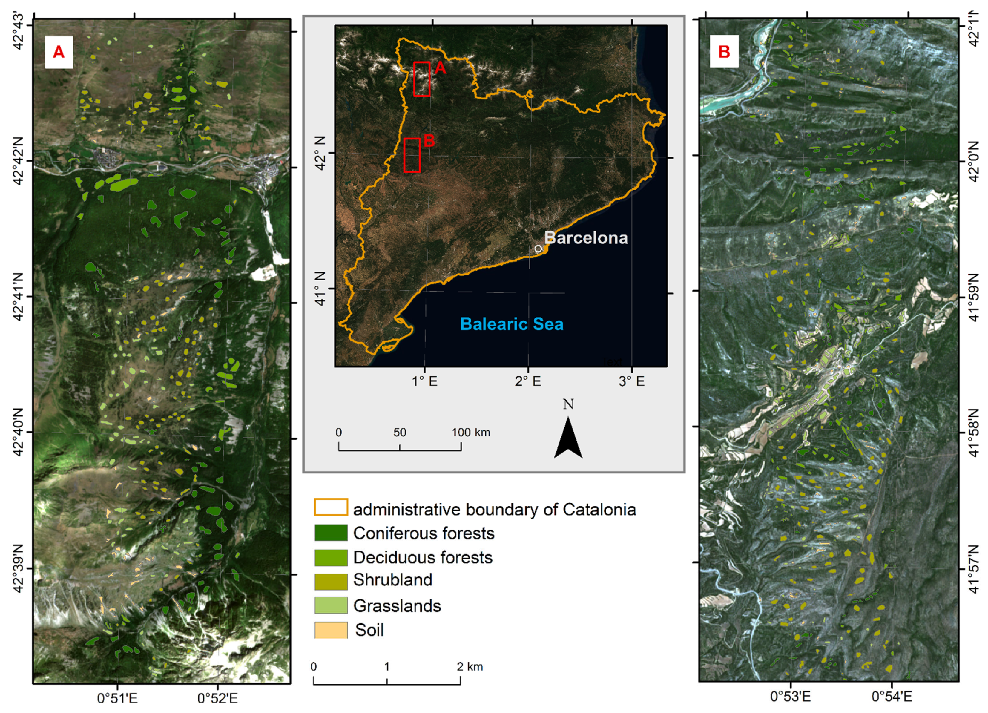
The research areas are located in two types of biogeographical places in Catalonia (southern Spain), labelled as A (an Atlantic vegetation type) and B (a Mediterranean vegetation; Figure 1; Figure 2). The A area (Valarties valley) is located in the Aran Valley (mountain Pyrenean region), which creates a special topo-climate due to its orography and Atlantic dominancy, and has rich and varied vegetation (forests, shrubby formations, sub-, and alpine meadows). The B area covers the mountain Montsec region (the pre-Pyrenees), which has a Mediterranean climate. The calcareous mountains cover 186.96 km2 (40 km long) and are catalogued as a natural park of the Natura 2000 Network: Special Protection Area (SPA) allowing coexistence with diversified flora (Serra del Montsec Protected Natural Area) [41]. The shrubby formations are formed mainly by shrubs (perennial woody plants not exceeding 5–8 m in height), and also include grasses, herbs, and geophytes, which can be natural, or sometimes anthropogenic (recovered vegetation after a fire). Natural shrubby formations occur in areas where factors, such as climate or soil, create conditions in which the growth of trees is prevented, but the growth of shrubs is possible.
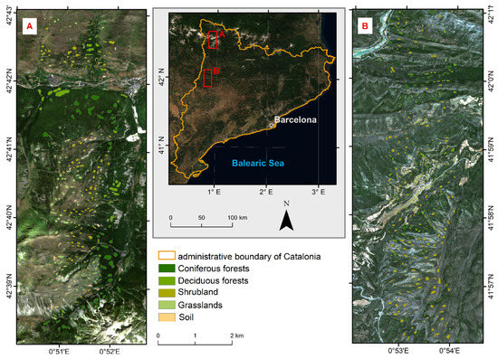
Figure 1.
Research area A (mountain Pyrenean region: the Valarties valley–an Atlantic vegetation type) and B (the pre-Pyrenees–Montsec region: a Mediterranean vegetation), in the background Sentinel-2 RGB 432 composition.

Figure 2.
Shrubby formations, on the left Pyrenean formations–A area (prostrate formations in the midst of grasslands and rocky areas); on the right pre-Pyrenean shrubs–B area. Authors’ pictures.
Shrubby formations are spread across the entire Catalan territory, from littoral to alpine areas, some of them labelled as habitats of communitary interest in the EU. In Corine Land Cover level 2, this formation is described as scrub and/or herbaceous vegetation associations (code 3.2; shrubby formation with single trees composed of dwarf forms of birch, willow and other species). However, on level 3 of the Corine land cover map–Transitional woodland-shrub was selected (code 324), and included different-size and condition trees, shrubs; herbaceous vegetation and natural bare surfaces (Transitional woodland/shrub) [42]. Under this physiognomic type are different botanical communities, and biodiversity is dynamically changing due to the spread to abandoned agricultural areas on the one hand, and the existence of fires on the other hand. Monitoring of such ecosystems is necessary in order calculate biovolumes to infer biomass, or CO2, as shrubs are involved in combustible models (calculating fire risk) and the modelling of post-fire shrub restoration in combination with soil analysis [43]. In the case of soil modelling, the second derivate transformation allows, by post-processing manipulation, for the identification of proper spectral properties [44,45].
2.2. Input data
Sentinel-2 and AISA airborne hyperspectral images that were atmospherically and geometrically corrected were used as input data. An AISA scanner was configured to acquire two-meter resolution for 256 bands (spectral range 394.04–997.43 nm, Table 1). Two AISA flight lines over NW Catalonia (Atlantic Pyrenees and pre-Pyrenees) were acquired on 24 July of 2019 and Sentinel-2 data (10 bands, Table 1) was captured the following day (25 July 2019; all images were cloud-free and good quality).

Table 1.
Input data used in the studies.
As additional data, the Land Cover Map of Catalonia, Topographical Map of Catalonia, Habitats Map of Catalonia and Digital Mapping Cameras DMC-3 Orthophotoimage was used as support material for correcting the training polygons that had been prepared for classification. It was also helpful for the visual verification of the classification results. The recent version of the Land Cover Map of Catalonia [46] was used, formerly El Mapa de Cobertes del Sòl de Catalunya MCSC (2009–2018), updated from 241 classes to 41. Topographical Map of Catalonia 1:5000 [47], accuracy: 1 m in planimetry and 1.5 m in altimetry. Habitats Map of Catalonia 1:50 000 [48] has extracted shrubland and grassland covers. Digital Mapping Cameras DMC-3 Orthophotoimage captured simultaneously with AISA images, 4 bands (infrared included), 45 cm of GSD. The Cartographic and Geological Institute of Catalonia generates, by correlation, a complete model for all of Catalonia, which is a high-resolution (1m) raster dataset. The DSM is created at 1-m resolution from aerial imagery using automatic image correlation methods. The DTM was derived from ICGC LiDAR (Light Detection and Ranging) coverage flights. Match-T/DSM automatically generated dense point clouds and digital terrain and surface models (DTM/DSM) from aerial image blocks. CHM was finally obtained by subtracting the ground surface (DTM) from the visible surface (DSM).
All of the above-mentioned materials allowed us to prepare training and verification (testing the classification results) polygons (45 polygons for each class), which were verified during a field reconnaissance (Table 2, Figure 3). The proportions between classes for each area vary, indicating an unbalanced dataset; therefore, each data set was balanced with a threshold of 200 pixels. The main reason for this is to give equal priority to each class during the training process [49,50].

Table 2.
Number of field-verified pixels for the polygons of the areas A and B.

Figure 3.
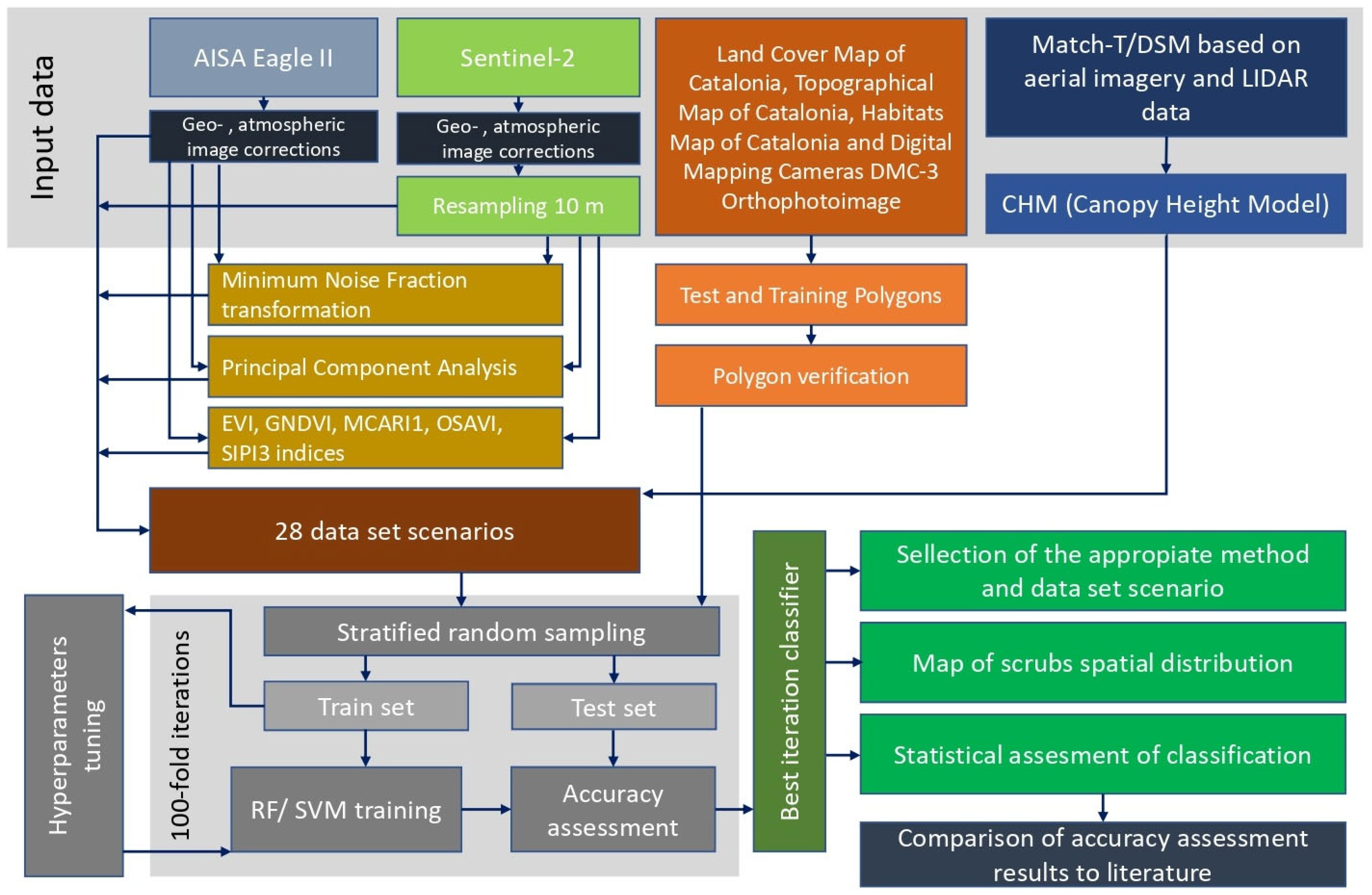
Analysis flow chart of multispectral and hyperspectral classifications.
The surface reflectivity is defined as the fraction of incident electromagnetic power that is reflected by the ground towards an observer and it is a function of radiation wavelength, but also of both illumination and observation geometry. The information contained in the radiometrically corrected images provided by the AISA Eagle II is essentially radiance, which is an indirect descriptor of surface properties, because it is the result of multiple interactions among the sun radiation, the atmosphere and the surface itself. The atmospheric correction is the part of the processing chain that compensates for the illumination and observation geometry dependences, and finally, provides the value of surface reflectivity for each hyperspectral band at pixel level. Briefly, for each pixel of the imaged scene, it considers both geometric and atmospheric information. The geometric part is essentially related to each pixel’s absolute coordinate and the position of the sun and the sensor in terms of azimuth and elevation when it was imaged. The atmospheric process considers the properties of the medium of propagation in terms of gas concentration, aerosols, column water vapor (CWV), etc., and is usually handled using an atmosphere simulator. For the correction of the AISA Eagle II data, version 5.0 of the MODerate resolution atmospheric TRANsmission (MODTRAN) software was used. In the case of the Sentinel-2 imagery, the atmospheric correction was performed by means of the Sen2Cor v2.8 [51] processor, which is freely distributed by the European Space Agency (ESA). Sen2Cor is a Level-2A processor which corrects single-date Sentinel-2 Level-1C Top-Of-Atmosphere (TOA) products from the effects of the atmosphere to a Level-2A Bottom-Of-Atmosphere (BOA) reflectance product. During the Sentinel-2 images correction, a 10 m × 10 m Digital Terrain Model (DTM; derived from aerial photogrammetry by the ICGC) was used in order to obtain a precise terrain correction, whereas for AISA, a DTM with 1 m resolution was used.
The research target was heterogeneous shrubby formation, which diversified spectrally due to their size, age and species, therefore, Canopy High Model (CHM) and remote sensing indices of vegetation were applied. Indices characterized canopy and condition of the vegetation (EVI) [31], chlorophyll concentration in vegetation (GNDVI) [52], relative abundance of chlorophyll (MCARI1) [53], cover of the vegetation with eliminated soil-induced variations in vegetation indices, allowing for the analysis of soil variation [54] and the measurement of the light absorption efficiency for photosynthesis (SIPI3, plant health and stress analysis) [55] (Table 3). Indices were selected on the basis of the literature, which indicates a wide spectrum of applications of the above-mentioned indices in the forest research [56,57,58] and shrubs [10,34] with the use of classifiers used in this study.

Table 3.
Remote sensing vegetation indices (VIs) calculated on Sentinel-2 and AISA data.
Due to additional sources of information, a preselection of spectral bands, especially in the case of hyperspectral images, was needed, therefore, Principal Component Analysis (PCA) and Minimum Noise Fraction (MNF) transformations were applied to reduce the number of spectral bands [59,60], which allowed for the addition of additional indices. Each of these dimensional reduction techniques works on a unique principle and has its own advantages and disadvantages. Researchers use single transformation techniques (PCA, MNF, ICA) or hybrid combinations of these techniques (PCA and ICA transforms performed on the MNF components) before classification, then compare the results [60], emphasizing that the transformation e.g., MNF allowed for the extraction of the most informative data, with high signal-to-noise ratio (SNR), especially in the first MNF bands [60,61]. In the case of PCA, bands are delivered as optimal data due to its maximized total variance from the original images [62]. According to researchers, MNF and PCA bands have great impact for an improvement of classification results [61,63] because PCA techniques work on the data variance, and MNF sorts the information based on the signal-to-noise ratio [60,64,65,66]. In the case of the AISA data, the first 15 MNF bands were highly decorrelated and used for classification, and in the case of MNF, there were the first four bands from the Sentinel-2 images (Table 4) and, respectively, four AISA’s PCA and three Sentinel-2’s PCA bands (Table 4).

Table 4.
The 28 scenarios were tested simultaneously on Sentinel-2 and AISA processed data and supporting materials like CHM, VIs or both of them; + data sets for the Sentinel-2, + data set for the AISA, with information how many bands was used for all data, MNF, PCA and the abbreviation name for the used VIs.
For the classification, a combination of all possible scenarios was tested to use both all spectral bands and remote sensing vegetation indices (in these scenarios, a significant improvement in the classification results was not expected, as the information contained in the indices was somewhat duplicated from the spectral bands). On the other hand, it was expected that the use of plant indices and transformed information contained in the MNF and PCA bands should not only accelerate the classification time due to the reduced amount of the input files, but also improve the classification accuracies, as data of different qualitative data were implemented in the procedure. An interesting element for testing was the effectiveness of the CHM; would those data allow for increased identification of the shrubs (do the bands contain sufficient spectral characteristics to classify this heterogenous formation with satisfactory accuracy?) Thus, for all the hyperspectral and multispectral images: all the bands, selected MNF or PCA bands and vegetation indices (VIs), were classified separately, each as a separate dataset. Then, each of these data sets were fused with CHM and calculated vegetation indices, or both of them, thereby creating a fused data set using Layer Stacking method. The following 28 scenarios were tested simultaneously on Sentinel-2 and AISA processed data and the supporting materials, CHM and VIs (Table 4).
2.3. The Classification Algorithm and Accuracy Assessment
RF and SVM classifiers were used in the R Studio 4.0.0; for this purpose, the raster [67], rgdal [68], randomForest [69] and e1071 packages [70] were implemented. The RF classifier is popular due to its low parameterization requirements and good classification results [71], offering better results than SVM in case of a lower amount of training pixels, e.g., 50–100 [72], noisy data or outliers [73,74,75]. This can be caused by multiple decision trees and randomized subsets [76]. In our case, signature pixel values representing different classes were selected from field-verified training polygons and randomized sampled (50:50) as training/validation patterns, limiting the phenomenon of overfitting during classification [77]. Each classification iteration used 500 trees (ntree parameter), which comes from the optimization process to obtain repetitive results [78,79]. The SVM, as a non-parametric classifier, allowed for a flexibility of training data, thus limiting errors and leading to high accuracy [28,80]. A radial basis function (RBF), due to its efficiency, was chosen [80,81] and also was recommended for Corine Land Cover classification (including 324 class–transitional woodland/shrub) [79]. The learning parameters were confirmed by the tuning process (gamma value of 0.1 and cost of 1000).
In this study, an iterative classification and accuracy assessment were applied (100 times repeated on randomized selected patterns). The results were assed based on the overall accuracy (OA), the Kappa coefficient [82], user accuracy (UA) and producer accuracy (PA) [83]. Based on the UA and PA, the values were calculated as an F1-score [84]. The final classification map was selected for each data set (AISA and Sentinel-2) based on the highest average F1-score results. For the visualization of the final maps, a 4x4-pixel filtration window was applied. This was to remove a large number of very small polygons, whose presence on small-scale maps disturbs the perception of the results (published maps), while the database contains all classified pixels and can be properly visible when zooming in on a given fragment of the map.
3. Results
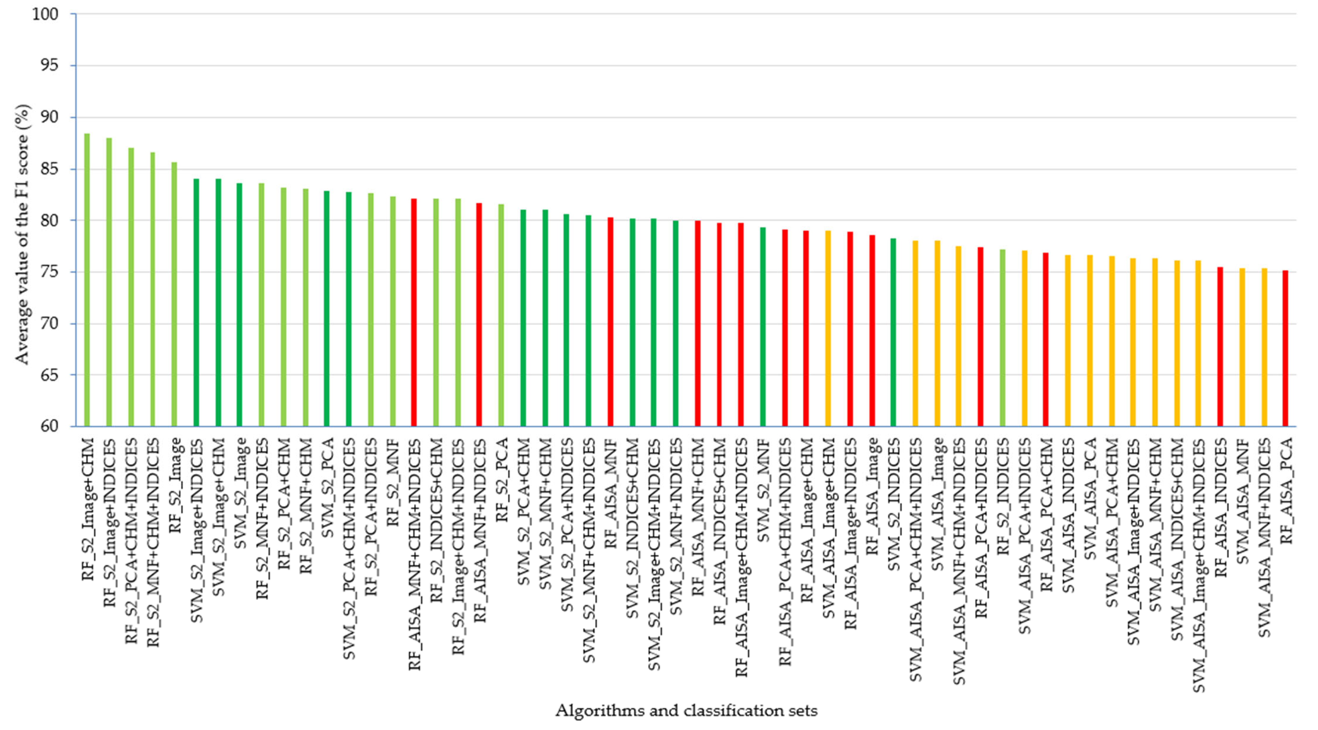
The highest results of the classification of the shrubland were achieved for the Sentinel-2 images and the RF classifier (88.46% of the average value of the F1-score for all classes and 91.86% of the F1-score for the scrubs area; the set of multispectral bands with CHM; Figure 4, Table 5). In the case of AISA imagery, the highest achieved mean value (82.15%) of F1-score was obtained for the all classes and 82.52% of F1-score for the scrubs area for the MNF with the vegetation indices combined with the canopy height model (Random Forest classifier, Table 5).
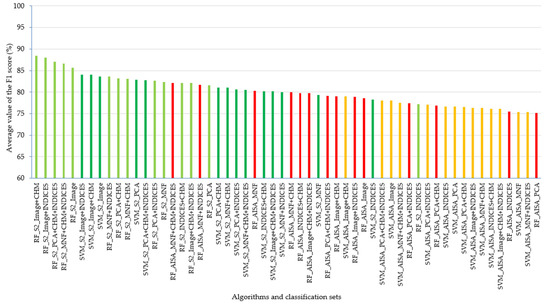
Figure 4.
The best classification results achieved from analyzed scenarios and classifiers: orange boxes mean SVM of AISA images, red—RF of AISA images, dark green—SVM of Sentinel-2, light green—RF of Sentinel-2 images.

Table 5.
Average values of: Overall Accuracy (OA), Kappa coefficient and F1-score for AISA and Sentinel-2 data sets.
In addition, it is relevant to note that the five best RF classification results of the shrubland apply to multispectral data, and have vegetation indices, MNF and CHM data sets. This is related to the diversity of shrubby formation, especially in combination with the 10-m pixel and the 2-m pixel for hyperspectral data. The higher classification accuracy values were obtained for the RF classifier, which means that with similar results, the computation process could be quicker than other options. Additional accuracy superiority for Sentinel-2 data over AISA is related to the range of AISA that was used for classification at the wavelength of 394.04–997.43 nm.
The aim of the research was to assess the potential of Sentinel-2 and AISA images, as well as RF and SVM classifiers, for shrubland mapping (analyzing all classes; Table 5); however, looking at the overall accuracy and Kappa coefficient results, the main focus is on the effectiveness of the analyzed classifier, which allows for the identification of all classes. Thus, it can be noticed that the Sentinel-2 data allowed for the obtainment of an average accuracy of 84.47% (regardless of whether RF or SVM was applied), and for AISA data, the accuracy was 79.04% (AISA images covered only the VNIR range). Looking at the results of classifiers, RF was slightly more effective (79.85% for AISA data, while for SVM, it was 78.23%), and Sentinel-2 data achieved 85.31% and 83.63%, respectively. In both analyzed hyperspectral and multispectral data sets, the highest results were obtained for the RF classifier. The average overall accuracy for the RF classifier for AISA data (all tested data sets) was 79.85%, with an average Kappa value of 0.73. The SVM classifier–78.23% for overall accuracy and 0.71 Kappa values, respectively. For the data sets for Sentinel-2, the RF classifier obtained an average overall accuracy of 85.32% (mean Kappa value for all sets 0.80), while the SVM classifier had an average overall accuracy of 83.63% (mean Kappa value for all sets 0.78; Table 5).
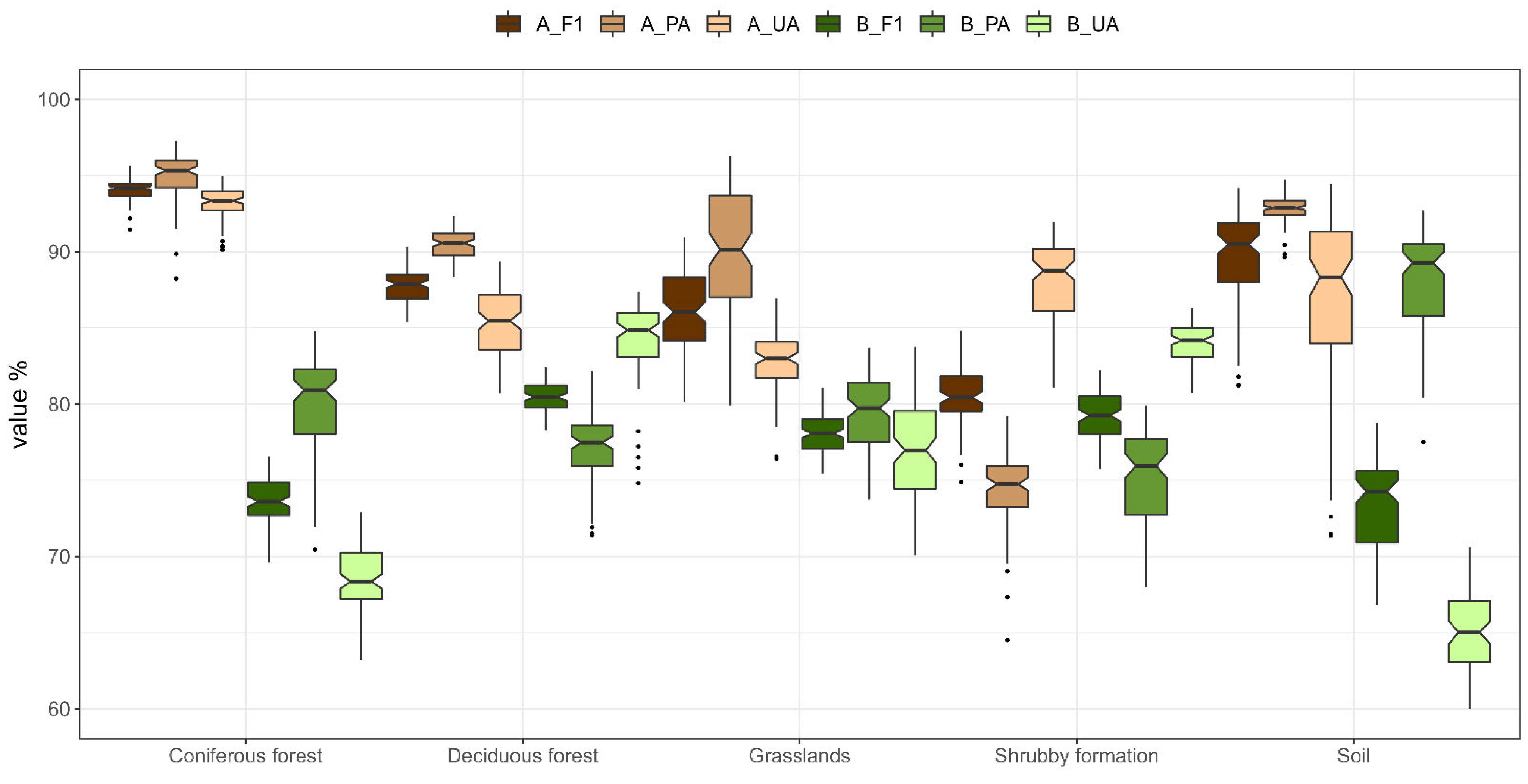
Shrubby classification results are differentiated for both areas A and B; the highest four data sets of AISA data contained MNF+CHM+INDICES; MNF+INDICES; MNF+CHM; MNF. Nevertheless, the best data set was selected – MNF+CHM+INDICES (based on F1-score and OA and Kappa values). The overall accuracy for area A was 90.44%, and for area B–78.55%, while for Kappa, the accuracies were 0.87 and 0.71, respectively. This differentiation is due to the variable surface forms of the area and their location in both areas. It is also worth emphasizing that shrubs often mix with grasslands or forests during classification, depending on their density. This caused a decrease of accuracies for the grassland, shrubby formations and deciduous forest classes (Figure 5).
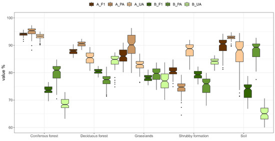
Figure 5.
The result for the RF classifier for MNF+CHM+INDICES data set for AISA in A and B area. F1-score; PA-Producer Accuracy; UA-User Accuracy; 100 iterations.
In the case of the shrubby identification on AISA hyperspectral data (MNF+CHM+Indices), it was noted that the results were closer in area A–82.83% than in B–82.20% F1-score (Figure 5). The class was mistaken for grasslands in both areas, and also in A area for deciduous and coniferous forest; while in B area, it was also mistaken for coniferous forest (similar spectral properties of the coverage of both classes; Table 6). In the case of Sentinel-2 data, a set of Image + CHM offered better results. The overall accuracy for the A area oscillated around 95.21%, and for B–85.01%, while for Kappa, the accuracies were 0.94 and 0.80, respectively. (Figure 6; Table 7).

Table 6.
Confusion matrix for A and B area for each class (RF and AISA_MNF+CHM+INDICES data set). Explanation: D.f.–Deciduous forest, C.f.–Coniferous forest.
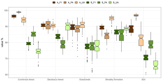
Figure 6.
The result for the RF classifier for Image+CHM data set for Sentinel-2 in A and B area. F1-score; PA–Producer Accuracy; UA–User Accuracy; 100 iterations.

Table 7.
Confusion matrix for A and B area for each class–the RF classifier for Image+CHM data set for Sentinel-2. Explanation: D.f.–Deciduous forest, C.f.–Coniferous forest.
Sentinel-2 images created with additional features (Image+CHM; Image+INDICES; MNF+CHM+INDICES; PCA+CHM+INDICES) optimal sets for shrubby formation mapping; but the highest scores were achieved for Sentinel-2 Image and CHM. Some shrub areas were misclassified in area A as deciduous forest and grasslands, and in area B, more as coniferous forest than grasslands (Figure 6, Table 7). This also confirms the same relationship in the matrices using the example of the classification results on AISA data discussed earlier.
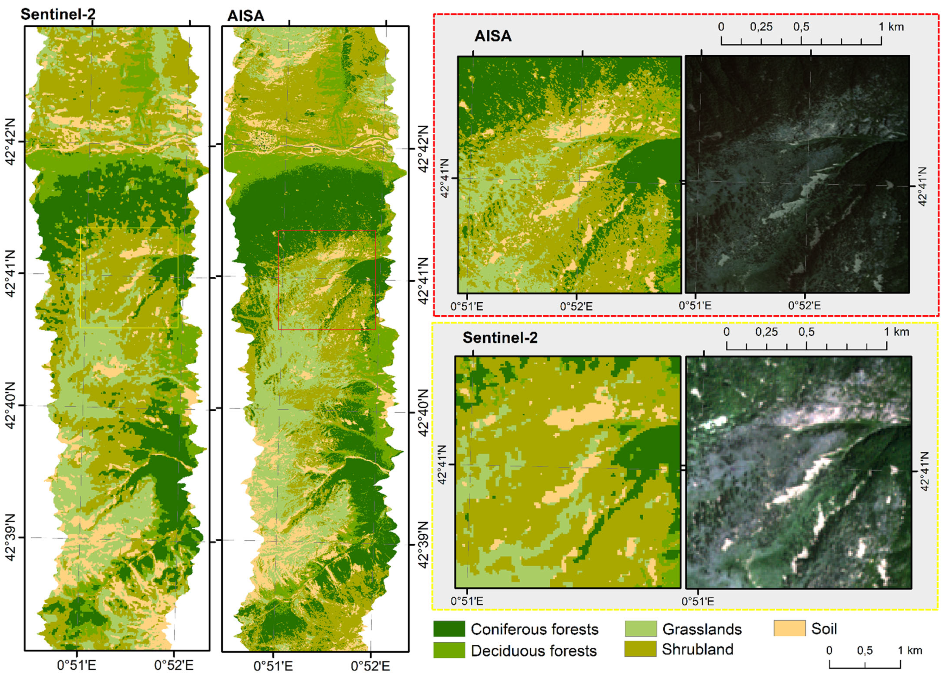
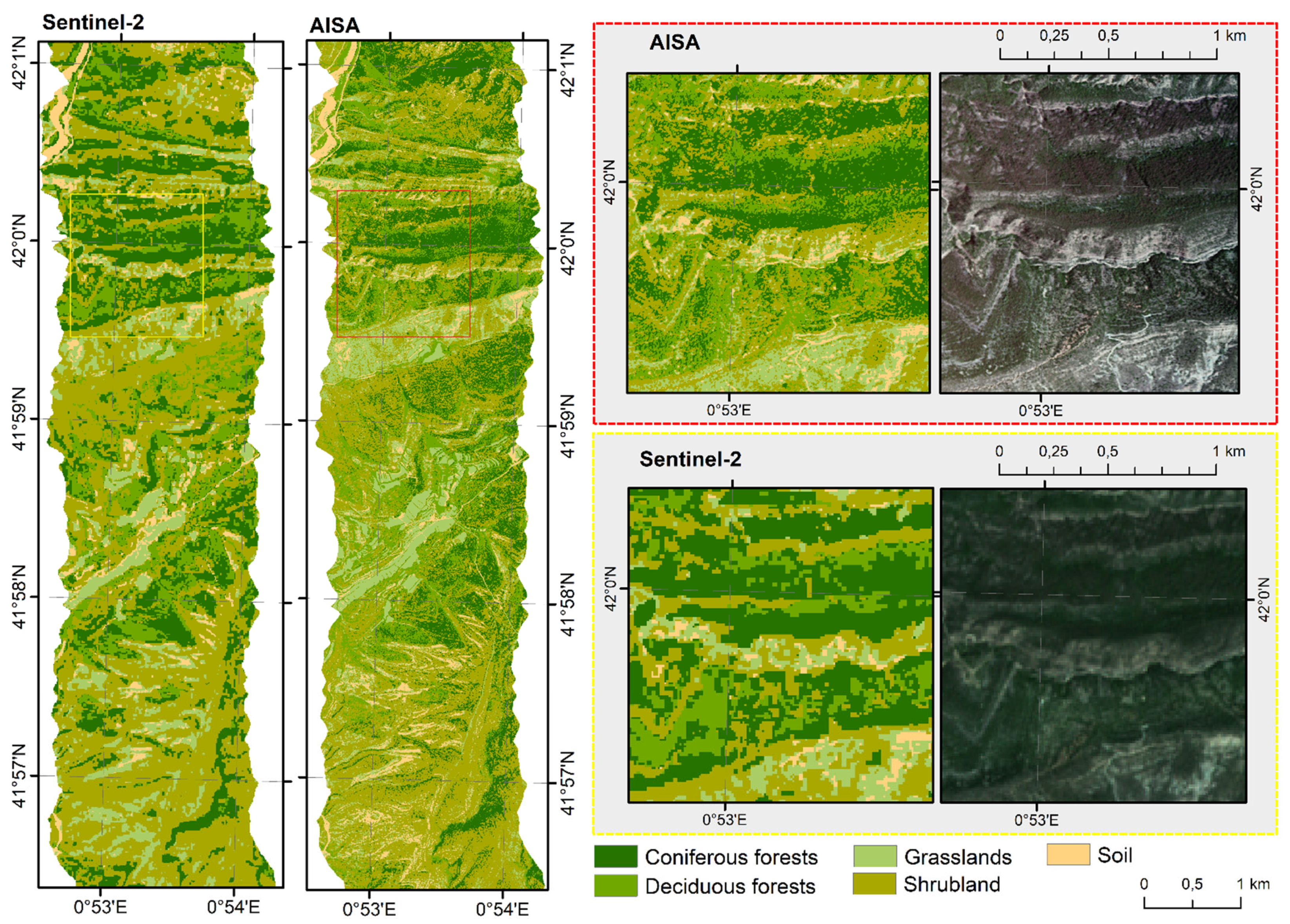
The classification of area A and B on Sentinel-2 data and AISA hyperspectral data gave a satisfactory result, and it was presented in the form of a map with approximated terrain segments for better visualization of the result (Figure 7 and Figure 8). Both areas were clipped to the same range for AISA data. Figure 7 shows the result for area A for both the Sentinel-2 data (Image + CHM data set) on the left side of the figure and the AISA data on the right side of the figure (MNF+CHM+INDICES data set). In addition, the approximate sections of the classified area for these two data cases are shown in the center. Figure 8 shows the same set of results for area B.
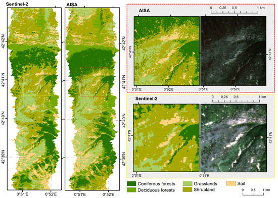
Figure 7.
Classification RF results for the Sentinel-2 (Images+CHM data set) and AISA data (MNF+CHM+INDICES data set) for the A area.

Figure 8.
Classification RF results for the Sentinel-2 (Image + CHM data set) and AISA data (MNF+CHM+INDICES data set) for the B area.
4. Discussion
Thus far, there have been not many studies on the identification of shrubby formation for the Mediterranean zone focusing on shrubby species. Due to the Corine Land Cover program, class 324 of transitional woodland/shrub is well-analyzed (Table 6). As an example, the outcomes of our team [79] highlighted the superiority of SVM RBF over the RF classifier, up to five percentage points, and Sentinel-2 images allowed for the identification of Catalonian transitional woodland/shrub (class 324) and sclerophyllous vegetation (323) with an average F1-score oscillating between 73% and 88% (F1-score achieved 80% for the 60 m resolution). In the case of the SVM RBF algorithm and multi-temporal Sentinel-2 images, the class 324 achieved OA: 76%, Kappa coefficient 0.74 [79]. In the present work, the average for both A and B areas’ F1-scores was ten percentage points higher because we focused on smaller, homogenous patterns of scrubs with original Sentinel-2 pixel sizes.
Our result of the classification of the Catalan shrubs on the Sentinel-2 images reached the highest values on all spectral bands–85.61% (F1-score, RF). Adding the vegetation indices, the accuracy increased to 88.46%, and for the image and CHM: 87.95%. Similar values were achieved based on MNF and PCA combinations. The SVM classifier achieved a few percentage points lower, as the highest was 84.01%. In the case of Portuguese shrubland, Aranha et al. [18] used the Minimum Distance classifier and Sentinel-2 data with 10 m resolution, and obtained very comparable results: 92% user accuracy and producer accuracy–84%, which corresponds to the F1-score value of 87.82%. The authors additionally recommended Sentinel-2’s B2, B3, B4 and B8 for the classification. In the conclusion, it was also emphasized that the studied biomass increased the fire hazard after the following five years [18]. As presented above, our results are better than those based on the similar vegetation indices, PCA and Tasseled Cap bands [22]; the authors mapped 24 Australian classes of scrubs vegetation based on Sentinel-2 data, and the SVM with the best accuracy was 72–74% [22].
The proposed solutions confirm that the obtained accuracy values are competitive in relation to the references (Table 8).

Table 8.
Comparison of the obtained results with achievements of other researchers.
The results of the classification also depend on the vegetation period in which the airborne data were acquired. It was confirmed that the optimal image acquisition period for plant communities mapping is from the second half of August to the first half of September in Central European vegetation periods, due to the complex physiognomy [13,14,15,78]. This was also confirmed by Calvão and Palmeirim [9], who observed a summer stress (an intense radiation and a water deficit), which changed the registered spectra of different types of vegetation included in the shrubby formations. It was also noted, as by previous researchers Gan et al. [16], that shrub land cover classification is not an easy task using remote sensing tools. In general, the shrub canopy is heterogeneous due to combinations with other targets (grasses, soil, single trees and shades), and an additional difficulty is the problematic separation of shrubs from grasslands, as they show similar spectral characteristics.
The optimization of tools and data allows for the use of Sentinel-2 data for constant monitoring of the shrubland cover, and also ensures regular repeatability according to the same conditions. This is extremely important for determining the fuel loads of the scrub extensions, models estimating biovolume, biomass and biophysical parameters of shrublands, and for the calculation of fire risk.
The proposed method, which is based on PCA/MNF bands, remote sensing indices, Canopy High Model data and Random Forest classifier, offered 5–20% higher accuracy than those obtained so far in the literature. It is important to highlight Sentinel-2’s dense time series, which allows it to compensate for its lower spectral and spatial resolution compared to the expensive, but much more accurate, airborne hyperspectral AISA data. Due to the high solar radiation and air temperatures, Mediterranean plants have a number of protective mechanisms depending on species, e.g., they are covered by waxes, or their leaves are smaller and change their position due to the sun’s radiation, which make their identification difficult because the woody parts and the soil generate mixel signals depend on shrub species. On the other hand, the shrubby formation provides a biodiversity and protects soil and living organisms from excessive overheating.
5. Conclusions
The present study confirmed a sufficient potential of Sentinel-2 and airborne AISA data to monitor the sensitive and heterogeneous ecosystem of the Mediterranean shrubland. Sentinel-2 images offer better results than AISA, but it should be remembered that the scope of hyperspectral data in this case concerned only visible and near infrared (VNIR) ranges. Outcomes of the Random Forest classifier indicated that differences between average values of the overall accuracies for all data sets amounted to a few percentage points (6–7%). Our research confirmed that remote sensing is the right tool to conduct permanent and objective monitoring, because:
- The shrubby formation was identified with an average overall accuracy above 91.86% based on the Sentinel-2 data; the best data set contained all bands + CHM and Random Forest as the classifier.
- AISA images offered 84.49% overall accuracy, the best data set: MNF + the vegetation indices (EVI, GNDVI, MCARI1, OSAVI, SIPI3) combined with the canopy height model and Random Forest classifier.
- Random Forest offered slightly better results than Support Vector Machine classifier; average overall accuracy for the SVM and AISA images (all tested data sets) was 78.23%, and for the RF: 79.85%. In the case of Sentinel-2, the SVM classifier obtained an average overall accuracy of 83.63%, while the RF classifier: 85.32%.
- We recommend the use of indices for characterizing the canopy and condition of the vegetation (EVI), chlorophyll concentration in vegetation (GNDVI), relative abundance of chlorophyll (MCARI1), cover of the vegetation with eliminated soil-induced variations in vegetation indices (OSAVI) and measure of the efficiency of which vegetation can use incident light for photosynthesis (SIPI3).
- Based on the results of the study and the literature review, the act of monitoring shrubby formation is ecologically important for monitoring water and for carbon management, as well as for preventing fires and soil erosion.
Author Contributions
Conceptualization, M.K. (Marlena Kycko), B.Z., A.T., L.P. and J.C.; methodology, M.K. (Marlena Kycko); validation, M.K. (Marlena Kycko), A.T., L.P. and J.C.; formal analysis, M.K. (Marlena Kycko); investigation, M.K. (Marlena Kycko); resources, J.C., V.P., M.K. (Marlena Kycko); writing—original draft preparation, M.K., B.Z., M.K. (Marcin Kluczek), L.P., A.T. and J.C.; writing—review and editing, all authors; visualization, M.K. (Marlena Kycko); supervision, M.K. (Marlena Kycko), B.Z. and J.C.; funding acquisition, M.K. (Marlena Kycko) and B.Z. All authors have read and agreed to the published version of the manuscript.
Funding
This research received funding (including publishing costs) from the European Union’s Horizon 2020 research and innovation program under the Marie Skłodowska-Curie grant agreement No. 734687 (H2020-MSCA-RISE-2016: innoVation in geospatial and 3D data—VOLTA) and the Polish Ministry of Education and Science (Ministerstwo Edukacji i Nauki—MEiN) in the framework of H2020 co-financed projects No. 3934/H2020/2018/2 and 379067/PnH/2017 for the period 2017–2022.
Data Availability Statement
Satellite Sentinel-2 data are publicly available online, images were acquired from the Copernicus Open Access Hub (https://scihub.copernicus.eu (accessed on 15 January 2019). Rest of used data including reference polygons were prepared and owned by ICGC Barcelona, which members are co-authors of the manuscript.
Acknowledgments
The authors express their gratitude to the editors and anonymous reviewers who contributed to the improvement of the article through their experience, work, and comments. The authors are also very grateful to the ICGC for providing reference data.
Conflicts of Interest
The authors declare no conflict of interest.
References
- Carreras, J.; Ferré, A.; Vigo, J. Manual dels Hàbitats de Catalunya; Generalitat de Catalunya, Departament de Territori i Sostenibilitat: Barcelona, Spain, 2015; p. 380. ISBN 978-84-393-9384-9. [Google Scholar]
- Mimeau, L.; Tramblay, Y.; Brocca, L.; Massari, C.; Camici, S.; Finaud-Guyot, P. Modeling the response of soil moisture to climate variability in the Mediterranean region. Hydrol. Earth Syst. Sci. 2021, 25, 653–669. [Google Scholar] [CrossRef]
- Mevy, J.-P.; Biryol, C.; Boiteau-Barral, M.; Miglietta, F. The Optical Response of a Mediterranean Shrubland to Climate Change: Hyperspectral Reflectance Measurements during Spring. Plants 2022, 11, 505. [Google Scholar] [CrossRef] [PubMed]
- Casermeiro, M.A.; Molina, J.A.; de la Cruz Caravaca, M.T.; Hernando Costa, J.; Hernando Massanet, M.I.; Moreno, P.S. Influence of scrubs on runoff and sediment loss in soils of Mediterranean climate. CATENA 2004, 57, 91–107. [Google Scholar] [CrossRef]
- Gratani, L.; Varone, L.; Ricotta, C.; Catoni, R. Mediterranean shrublands carbon sequestration: Environmental and economic benefits. Mitig. Adapt. Strateg. Glob. Chang. 2013, 18, 1167–1182. [Google Scholar] [CrossRef]
- Farguell, J.; Ubeda, X.; Pacheco, E. Shrub removal effects on runoff and sediment transport in a mediterranean experimental catchment (Vernega River, NE Spain). CATENA 2022, 210, 105882. [Google Scholar] [CrossRef]
- Torre, I.; Jaime-González, C.; Díaz, M. Habitat Suitability for Small Mammals in Mediterranean Landscapes: How and Why Shrubs Matter. Sustainability 2022, 14, 1562. [Google Scholar] [CrossRef]
- Underwood, E.C.; Viers, J.H.; Klausmeyer, K.R.; Cox, R.L.; Shaw, M.R. Threats and biodiversity in the mediterranean biome. Divers. Distrib. 2009, 15, 188–197. [Google Scholar] [CrossRef]
- Calvao, T.; Palmeirim, J.M. Mapping Mediterranean scrub with satellite imagery: Biomass estimation and spectral behaviour. Int. J. Remote Sens. 2004, 25, 3113–3126. [Google Scholar] [CrossRef]
- Calvão, T.; Palmeirim, J.M. A comparative evaluation of spectral vegetation indices for the estimation of biophysical characteristics of Mediterranean semi-deciduous shrub communities. Int. J. Remote Sens. 2011, 32, 2275–2296. [Google Scholar] [CrossRef]
- Zagajewski, B.; Tømmervik, H.; Bjerke, J.W.; Raczko, E.; Bochenek, Z.; Kłos, A.; Jarocińska, A.; Lavender, S.; Ziółkowski, D. Intraspecific Differences in Spectral Reflectance Curves as Indicators of Reduced Vitality in High-Arctic Plants. Remote Sens. 2017, 9, 1289. [Google Scholar] [CrossRef]
- Zagajewski, B.; Kycko, M.; Tømmervik, H.; Bochenek, Z.; Wojtuń, B.; Bjerke, J.W.; Kłos, A. Feasibility of hyperspectral vegetation indices for the detection of chlorophyll concentration in three high Arctic plants: Salix polaris, Bistorta vivipara, and Dryas octopetala. Acta Soc. Bot. Pol. 2018, 87, 3604. [Google Scholar] [CrossRef]
- Kycko, M.; Zagajewski, B.; Zwijacz-Kozica, M.; Cierniewski, J.; Romanowska, E.; Orłowska, K.; Ochtyra, A.; Jarocińska, A. Assessment of Hyperspectral Remote Sensing for Analyzing the Impact of Human Trampling on Alpine Swards. Mt. Res. Dev. 2017, 37, 66–74. [Google Scholar] [CrossRef]
- Kycko, M.; Zagajewski, B.; Lavender, S.; Romanowska, E.; Zwijacz-Kozica, M. The Impact of Tourist Traffic on the Condition and Cell Structures of Alpine Swards. Remote Sens. 2018, 10, 220. [Google Scholar] [CrossRef]
- Kycko, M.; Zagajewski, B.; Lavender, S.; Dabija, A. In Situ Hyperspectral Remote Sensing for Monitoring of Alpine Trampled and Recultivated Species. Remote Sens. 2019, 11, 1296. [Google Scholar] [CrossRef]
- Gan, L.; Cao, X.; Chen, X.; He, Q.; Cui, X.; Zhao, C. Mapping Shrub Coverage in Xilin Gol Grassland with Multi-Temporal Sentinel-2 Imagery. Remote Sens. 2022, 14, 3266. [Google Scholar] [CrossRef]
- Waśniewski, A.; Hościło, A.; Zagajewski, B.; Moukétou-Tarazewicz, D. Assessment of Sentinel-2 Satellite Images and Random Forest Classifier for Rainforest Mapping in Gabon. Forests 2020, 11, 941. [Google Scholar] [CrossRef]
- Aranha, J.; Enes, T.; Calvão, A.; Viana, H. Shrub Biomass Estimates in Former Burnt Areas Using Sentinel 2 Images Processing and Classification. Forests 2020, 11, 555. [Google Scholar] [CrossRef]
- Nunes, L.; Pasalodos-Tato, M.; Alberdi, I.; Sequeira, A.C.; Vega, J.A.; Silva, V.; Vieira, P.; Rego, F.C. Bulk Density of Shrub Types and Tree Crowns to Use with Forest Inventories in the Iberian Peninsula. Forests 2022, 13, 555. [Google Scholar] [CrossRef]
- Vega, J.A.; Arellano-Pérez, S.; Álvarez-González, J.G.; Fernández, C.; Jiménez, E.; Fernández-Alonso, J.M.; Vega-Nieva, J.; Briones-Herrera, C.; Alonso-Rego, C.; Fontúrbel, T.; et al. Modelling aboveground biomass and fuel load components at stand level in shrub communities in NW Spain. For. Ecol. Manag. 2022, 505, 119926. [Google Scholar] [CrossRef]
- Fassnacht, F.E.; Poblee-Olivares, J.; Rivero, L.; Lopatin, J.; Ceballos-Comisso, A.; Galleguillos, M. Using Sentinel-2 and canopy height models to derive a landscape-level biomass map covering multiple vegetation types. Int. J. Appl. Earth Obs. Geoinf. 2021, 94, 102236. [Google Scholar] [CrossRef]
- Macintyre, P.; van Niekerk, A.; Mucina, L. Efficacy of multi-season Sentinel-2 imagery for compositional vegetation classification. Int. J. Appl. Earth Obs. Geoinf. 2020, 85, 101980. [Google Scholar] [CrossRef]
- Sequeira, I.A.H. Landcover and Crop Type Classification with Intra-Annual Times Series of Sentinel-2 and Machine Learning at Central Portugal. Master’s Thesis, Universidade Nova de Lisboa, Lisboa, Portugal, 28 February 2020. [Google Scholar]
- Khodadadzadeh, M.; Li, J.; Prasad, S.; Plaza, A. Fusion of Hyperspectral and LiDAR Remote Sensing Data Using Multiple Feature Learning. IEEE J. Sel. Top. Appl. Earth Obs. Remote Sens. 2015, 8, 2971–2983. [Google Scholar] [CrossRef]
- Nasrabadi, N.M. Kernel-Based Spectral Matched Signal Detectors for Hyperspectral Target Detection. In Proceedings of the Lecture Notes in Computernat Scional Conference on Pattern Recognition and Machine Intelligence, Kolkata, India, 18–22 December 2007; pp. 67–76. [Google Scholar]
- Kwan, C.; Gribben, D.; Ayhan, B.; Li, J.; Bernabe, S.; Plaza, A. An Accurate Vegetation and Non-Vegetation Differentiation Approach Based on Land Cover Classification. Remote Sens. 2020, 12, 3880. [Google Scholar] [CrossRef]
- Zhang, C.; Xie, Z. Object-based Vegetation Mapping in the Kissimmee River Watershed Using HyMap Data and Machine Learning Techniques. Wetlands 2013, 33, 233–244. [Google Scholar] [CrossRef]
- Burai, P.; Deák, B.; Valkó, O.; Tomor, T. Classification of Herbaceous Vegetation Using Airborne Hyperspectral Imagery. Remote Sens. 2015, 7, 2046–2066. [Google Scholar] [CrossRef]
- Raczko, E.; Zagajewski, B. Tree species classification of the UNESCO Man and the Biosphere Karkonoski National Park (Poland) using artificial neural networks and APEX hyperspectral images. Remote Sens. 2018, 10, 1111. [Google Scholar] [CrossRef]
- Kupková, L.; Červená, L.; Suchá, R.; Jakešová, L.; Zagajewski, B.; Březina, S.; Albrechtová, J. Classification of Tundra Vegetation in the Krkonoše Mts. National Park Using APEX, AISA Dual and Sentinel-2A Data. Eur. J. Remote Sens. 2017, 50, 29–46. [Google Scholar] [CrossRef]
- Huete, A. A comparison of vegetation indices over a global set of TM images for EOS-MODIS. Remote Sens. Environ. 1997, 59, 440–451. [Google Scholar] [CrossRef]
- Huete, A.; Didan, K.; Miura, T.; Rodriguez, E.; Gao, X.; Ferreira, L. Overview of the radiometric and biophysical performance of the MODIS vegetation indices. Remote Sens. Environ. 2002, 83, 195–213. [Google Scholar] [CrossRef]
- Pu, R.; Gong, P.; Tian, Y.; Miao, X.; Carruthers, R.I.; Anderson, G.L. Using classification and NDVI differencing methods for monitoring sparse vegetation coverage: A case study of saltcedar in Nevada, USA. Int. J. Remote Sens. 2008, 29, 3987–4011. [Google Scholar] [CrossRef]
- Olsson, A.D.; Van Leeuwen, W.J.D.; Marsh, S.E. Feasibility of Invasive Grass Detection in a Desertscrub Community Using Hyperspectral Field Measurements and Landsat TM Imagery. Remote Sens. 2011, 3, 2283–2304. [Google Scholar] [CrossRef]
- Valderrama-Landeros, L.; Flores-de-Santiago, F.; Kovacs, J.M.; Flores-Verdugo, F. An assessment of commonly employed satellite-based remote sensors for mapping mangrove species in Mexico using an NDVI-based classification scheme. Environ. Monit. Assess. 2018, 190, 23. [Google Scholar] [CrossRef] [PubMed]
- Kopeć, D.; Sabat-Tomala, A.; Michalska-Hejduk, D.; Jarocińska, A.; Niedzielko, J. Application of airborne hyperspectral data for mapping of invasive alien Spiraea tomentosa L.: A serious threat to peat bog plant communities. Wetl. Ecol. Manag. 2020, 28, 357–373. [Google Scholar] [CrossRef]
- Szostak, M.; Likus-Cieślik, J.; Pietrzykowski, M. PlanetScope Imageries and LiDAR Point Clouds Processing for Automation Land Cover Mapping and Vegetation Assessment of a Reclaimed Sulfur Mine. Remote Sens. 2021, 13, 2717. [Google Scholar] [CrossRef]
- Sheykhmousa, M.; Mahdianpari, M.; Ghanbari, H.; Mohammadimanesh, F.; Ghamisi, P.; Homayouni, S. Support Vector Machine Versus Random Forest for Remote Sensing Image Classification: A Meta-Analysis and Systematic Review. IEEE J. Sel. Top. Appl. Earth Obs. Remote Sens. 2020, 13, 6308–6325. [Google Scholar] [CrossRef]
- Bayle, A.; Carlson, B.Z.; Thierion, V.; Isenmann, M.; Choler, P. Improved Mapping of Mountain Shrublands Using the Sentinel-2 Red-Edge Band. Remote Sens. 2019, 11, 2807. [Google Scholar] [CrossRef]
- Gitelson, A.A.; Merzlyak, M.N. Non-destructive assessment of chlorophyll carotenoid and anthocyanin content in higher plant leaves: Principles and algorithms. Remote Sens. Agric. Environ. 2004, 263, 78–94. [Google Scholar]
- Serra del Montsec Protected Natural Area. Available online: http://www.catalunya.com/serra-del-montsec-protected-natural-area-17-17001-15?language=en (accessed on 2 March 2020).
- Transitional Woodland/Shrub. Available online: https://land.copernicus.eu/user-corner/technical-library/corine-land-cover-nomenclature-guidelines/html/index-clc-324.html (accessed on 2 March 2020).
- García Matallana, R.; Lucas-Borja, M.E.; Gómez-Sánchez, M.E.; Uddin, S.M.M.; Zema, D.A. Post-fire restoration effectiveness using two soil preparation techniques and different shrubs species in pine forests of South-Eastern Spain. Ecol. Eng. 2022, 178, 106579. [Google Scholar] [CrossRef]
- Cierniewski, J.; Kazmierowski, C.; Krolewicz, S.; Piekarczyk, J.; Wrobel, M.; Zagajewski, B. Effects of Different Illumination and Observation Techniques of Cultivated Soils on Their Hyperspectral Bidirectional Measurements Under Field and Laboratory Conditions. IEEE J. Sel. Top. Appl. Earth Obs. Remote Sens. 2014, 7, 2525–2530. [Google Scholar] [CrossRef]
- Cierniewski, J.; Ceglarek, J.; Karnieli, A.; Królewicz, S.; Kaźmierowski, C.; Zagajewski, B. Predicting the diurnal blue-sky albedo of soils using their laboratory reflectance spectra and roughness indices. J. Quant. Spectrosc. Radiat. Transf. 2017, 200, 25–31. [Google Scholar] [CrossRef]
- Land Cover Map of Catalonia. Available online: https://www.creaf.uab.es/mcsc/usa/index.htm (accessed on 2 March 2020).
- Topographical Map of Catalonia 1:5000. Available online: https://www.icgc.cat/en/Downloads/Maps-in-image-format/Topographic-map-1-5-000 (accessed on 2 March 2020).
- Habitats Map of Catalonia 1:50,000. Available online: https://www.ub.edu/geoveg/en/mapes.php#hab (accessed on 2 March 2020).
- Zagajewski, B.; Kluczek, M.; Raczko, E.; Njegovec, A.; Dabija, A.; Kycko, M. Comparison of Random Forest, Support Vector Machines, and Neural Networks for Post-Disaster Forest Species Mapping of the Krkonoše/Karkonosze Transboundary Biosphere Reserve. Remote Sens. 2021, 13, 2581. [Google Scholar] [CrossRef]
- Migas-Mazur, R.; Kycko, M.; Zwijacz-Kozica, T.; Zagajewski, B. Assessment of Sentinel-2 Images, Support Vector Machines and Change Detection Algorithms for Bark Beetle Outbreaks Mapping in the Tatra Mountains. Remote Sens. 2021, 13, 3314. [Google Scholar] [CrossRef]
- Sen2cor v2.8. Available online: https://step.esa.int/main/snap-supported-plugins/sen2cor/sen2cor_v2-8/ (accessed on 3 March 2020).
- Gitelson, A.A.; Kaufman, Y.J.; Merzlyak, M.N. Use of a green channel in remote sensing of global vegetation from EOS-MODIS. Remote Sens. Environ. 1996, 58, 289–298. [Google Scholar] [CrossRef]
- Haboudane, D. Hyperspectral vegetation indices and novel algorithms for predicting green LAI of crop canopies: Modeling and validation in the context of precision agriculture. Remote Sens. Environ. 2004, 90, 337–352. [Google Scholar] [CrossRef]
- Rondeaux, G.; Steven, M.; Baret, F. Optimization of soil-adjusted vegetation indices. Remote Sens. Environ. 1996, 55, 95–107. [Google Scholar] [CrossRef]
- Penuelas, J.; Baret, F.; Filella, I. Semiempirical Indexes to Assess Carotenoids Chlorophyll-a Ratio from Leaf Spectral Reflectance. Photosynthetica 1995, 31, 221–230. [Google Scholar]
- Xue, J.; Su, B. Significant Remote Sensing Vegetation Indices: A Review of Developments and Applications. J. Sens. 2017, 2017, 1353691. [Google Scholar] [CrossRef]
- Knauer, U.; von Rekowski, C.S.; Stecklina, M.; Krokotsch, T.; Pham Minh, T.; Hauffe, V.; Kilias, D.; Ehrhardt, I.; Sagischewski, H.; Chmara, S.; et al. Tree Species Classification Based on Hybrid Ensembles of a Convolutional Neural Network (CNN) and Random Forest Classifiers. Remote Sens. 2019, 11, 2788. [Google Scholar] [CrossRef]
- Macedo, F.L.; Sousa, A.M.O.; Gonçalves, A.C.; Marques da Silva, J.R.; Mesquita, P.A.; Rodrigues, R.A.F. Above-ground biomass estimation for Quercus rotundifolia using vegetation indices derived from high spatial resolution satellite images. Eur. J. Remote Sens. 2018, 51, 932–944. [Google Scholar] [CrossRef]
- Kruse, F.A.; Kim, A.M.; Runyon, S.C.; Carlisle, S.C.; Clasen, C.C.; Esterline, C.H.; Jalobeanu, A.; Metcalf, J.P.; Basgall, P.L.; Trask, D.M.; et al. Multispectral, hyperspectral, and LiDAR remote sensing and geographic information fusion for improved earthquake response. In Proceedings of the Algorithms and Technologies for Multispectral, Hyperspectral, and Ultraspectral Imagery XX; Velez-Reyes, M., Kruse, F.A., Eds.; SPIE Defense + Security: Baltimore, MD, USA, 2014; p. 90880K. [Google Scholar] [CrossRef]
- Sahithi, V.S.; Krishna, I.V.M. Performance evaluation of dimensionality reduction techniques on CHRIS hyperspectral data for surface discrimination. J. Geomat. 2016, 10, 7–11. [Google Scholar]
- Priyadarshini, K.N.; Sivashankari, V.; Shekhar, S.; Balasubramani, K. Comparison and Evaluation of Dimensionality Reduction Techniques for Hyperspectral Data Analysis. Proceedings 2019, 24, 6. [Google Scholar] [CrossRef]
- Martel, E.; Lazcano, R.; López, J.; Madroñal, D.; Salvador, R.; López, S.; Juarez, E.; Guerra, R.; Sanz, C.; Sarmiento, R. Implementation of the Principal Component Analysis onto High-Performance Computer Facilities for Hyperspectral Dimensionality Reduction: Results and Comparisons. Remote Sens. 2018, 10, 864. [Google Scholar] [CrossRef]
- Carvalho Júnior, O.A.; Carvalho, A.P.F.; Meneses, P.R.; Guimarães, R.F. Classificação e eliminação dos ruídos em imagens hiperespectrais pela análise seqüencial da transformação por Fração de Ruído Mínima. Rev. Bras. Geofísica 2002, 20, 31–41. [Google Scholar] [CrossRef][Green Version]
- Green, A.A.; Berman, M.; Switzer, P.; Craig, M.D. A transformation for ordering multispectral data in terms of image quality with implications for noise removal. IEEE Trans. Geosci. Remote Sens. 1988, 26, 65–74. [Google Scholar] [CrossRef]
- Chatziantoniou, A.; Psomiadis, E.; Petropoulos, G.P. Co-Orbital Sentinel 1 and 2 for LULC Mapping with Emphasis on Wetlands in a Mediterranean Setting Based on Machine Learning. Remote Sens. 2017, 9, 1259. [Google Scholar] [CrossRef]
- Zhang, L.; Su, H.; Shen, J. Hyperspectral Dimensionality Reduction Based on Multiscale Superpixelwise Kernel Principal Component Analysis. Remote Sens. 2019, 11, 1219. [Google Scholar] [CrossRef]
- Hijmans, R.J. Raster: Geographic Data Analysis and Modeling. R Package Version 3.3-13. 2020. Available online: https://rdrr.io/cran/raster/ (accessed on 25 April 2020).
- Bivand, R.; Keitt, T.; Rowlingson, B. Rgdal: Bindings for the ‘Geospatial’ Data Abstraction Library. R Package Version 1.5-12. 2020. Available online: https://rdrr.io/cran/rgdal/ (accessed on 25 April 2020).
- Liaw, A.; Wiener, M. RandomForest: Classification and Regression by randomForest. R News 2002, 2, 18–22. Available online: https://rdrr.io/cran/randomForest/ (accessed on 25 April 2020).
- Meyer, D.; Dimitriadou, E.; Hornik, K.; Weingessel, A.; Leisch, F. e1071: Misc Functions of the Department of Statistics, Probability Theory Group; (Formerly: E1071); R Package Version 1.7-3; TU: Wien, Austria, 2019; Available online: https://rdrr.io/rforge/e1071/ (accessed on 25 April 2020).
- Chutia, D.; Bhattacharyya, D.K.; Sarma, K.K.; Kalita, R.; Sudhakar, S. Hyperspectral Remote Sensing Classifications: A Perspective Survey. Trans. GIS 2016, 20, 463–490. [Google Scholar] [CrossRef]
- Kluczek, M.; Zagajewski, B.; Kycko, M. Airborne HySpex hyperspectral versus multitemporal Sentinel-2 images for mountain plant communities mapping. Remote Sens. 2022, 14, 1209. [Google Scholar] [CrossRef]
- Rodriguez-Galiano, V.F.; Ghimire, B.; Rogan, J.; Olmo, M.C.; Rigol-Sanchez, J.P. An assessment of the effectiveness of a random forest classifier for land-cover classification. ISPRS J. Photogramm. Remote Sens. 2012, 67, 93–104. [Google Scholar] [CrossRef]
- Pelletier, C.; Valero, S.; Inglada, J.; Champion, N.; Sicre, C.M.; Dedieu, G. Effect of Training Class Label Noise on Classification Performances for Land Cover Mapping with Satellite Image Time Series. Remote Sens. 2017, 9, 173. [Google Scholar] [CrossRef]
- Sławik, Ł.; Niedzielko, J.; Kania, A.; Piórkowski, H.; Kopeć, D. Multiple Flights or Single Flight Instrument Fusion of Hyperspectral and ALS Data? A Comparison of their Performance for Vegetation Mapping. Remote Sens. 2019, 11, 970. [Google Scholar] [CrossRef]
- Breiman, L. Random Forests. Mach. Learn. 2001, 45, 5–32. [Google Scholar] [CrossRef]
- Breiman, L. Prediction Games and Arcing Algorithms. Neural Comput. 1999, 11, 1493–1517. [Google Scholar] [CrossRef]
- Sabat-Tomala, A.; Raczko, E.; Zagajewski, B. Mapping Invasive Plant Species with Hyperspectral Data Based on Iterative Accuracy Assessment Techniques. Remote Sens. 2022, 14, 64. [Google Scholar] [CrossRef]
- Dabija, A.; Kluczek, M.; Zagajewski, B.; Raczko, E.; Kycko, M.; Al-Sulttani, A.H.; Tardà, A.; Pineda, L.; Corbera, J. Comparison of Support Vector Machines and Random Forests for Corine Land Cover Mapping. Remote Sens. 2021, 13, 777. [Google Scholar] [CrossRef]
- Marcinkowska–Ochtyra, A.; Zagajewski, B.; Raczko, E.; Ochtyra, A.; Jarocińska, A. Classification of High-Mountain Vegetation Communities within a Diverse Giant Mountains Ecosystem Using Airborne APEX Hyperspectral Imagery. Remote Sens. 2018, 10, 570. [Google Scholar] [CrossRef]
- Melgani, F.; Bruzzone, L. Classification of hyperspectral remote sensing images with support vector machines. IEEE Trans. Geosci. Remote Sens. 2004, 42, 1778–1790. [Google Scholar] [CrossRef]
- Cohen, J. A Coefficient of Agreement for Nominal Scales. Educ. Psychol. Meas. 1960, 20, 37–46. [Google Scholar] [CrossRef]
- Lillesand, T.; Kiefer, R.; Chipman, J. Remote Sensing and Image Interpretation, 7th ed.; Wiley: Hoboken, NJ, USA, 2015; p. 736. ISBN 978-1-118-34328-9. [Google Scholar]
- Sasaki, Y. The truth of the F-measure. Teach. Tutor Mater. 2007, 1, 1–5. [Google Scholar]
- Carbonell-Rivera, J.P.; Torralba, J.; Estornell, J.; Ruiz, L.Á.; Crespo-Peremarch, P. Classification of Mediterranean Shrub Species from UAV Point Clouds. Remote Sens. 2022, 14, 199. [Google Scholar] [CrossRef]
- Venter, Z.S.; Sydenham, M.A.K. Continental-Scale Land Cover Mapping at 10 m Resolution Over Europe (ELC10). Remote Sens. 2021, 13, 2301. [Google Scholar] [CrossRef]
- Li, Z.; Ding, J.; Zhang, H.; Feng, Y. Classifying Individual Shrub Species in UAV Images—A Case Study of the Gobi Region of Northwest China. Remote Sens. 2021, 13, 4995. [Google Scholar] [CrossRef]
- Listiani, I.A. Mediterranean Shrub Classification Using Multi-Temporal Multi-Spectral Satellite Images. Master’s Thesis, Middle East Technical University, Ankara, Turkey, 12 February 2021. [Google Scholar]
- Paz-Kagan, T.; Chang, J.G.; Shoshany, M.; Sternberg, M.; Karnieli, A. Assessment of plant species distribution and diversity along a climatic gradient from Mediterranean woodlands to semi-arid shrublands. GISci. Remote Sens. 2021, 58, 929–953. [Google Scholar] [CrossRef]
- Ayhan, B.; Kwan, C. Tree, Shrub, and Grass Classification Using Only RGB Images. Remote Sens. 2020, 12, 1333. [Google Scholar] [CrossRef]
- Gudmann, A.; Csikós, N.; Szilassi, P.; Mucsi, L. Improvement in Satellite Image-Based Land Cover Classification with Landscape Metrics. Remote Sens. 2020, 12, 3580. [Google Scholar] [CrossRef]
- Hernandez, I.; Benevides, P.; Costa, H.; Caetano, M. Exploring Sentinel-2 for land cover and crop mapping in Portugal. Int. Arch. Photogramm. Remote Sens. Spat. Inf. Sci. 2020, XLIII-B3-2, 83–89. [Google Scholar] [CrossRef]
- Zhang, M.; Huang, H.; Li, Z.; Hackman, K.O.; Liu, C.; Andriamiarisoa, R.L.; Ny Aina Nomenjanahary Raherivelo, T.; Li, Y.; Gong, P. Automatic High-Resolution Land Cover Production in Madagascar Using Sentinel-2 Time Series, Tile-Based Image Classification and Google Earth Engine. Remote Sens. 2020, 12, 3663. [Google Scholar] [CrossRef]
- Xie, Z.; Chen, Y.; Lu, D.; Li, G.; Chen, E. Classification of Land Cover, Forest, and Tree Species Classes with ZiYuan-3 Multispectral and Stereo Data. Remote Sens. 2019, 11, 164. [Google Scholar] [CrossRef]
- Adams, B.T.; Matthews, S.N. Enhancing Forest and Shrubland Mapping in a Managed Forest Landscape with Landsat–LiDAR Data Fusion. Nat. Areas J. 2018, 38, 402–418. [Google Scholar] [CrossRef]
- Fragoso-Campón, L.; Quirós, E.; Mora, J.; Gutiérrez, J.A.; Durán-Barroso, P. Accuracy Enhancement for Land Cover Classification Using LiDAR and Multitemporal Sentinel 2 Images in a Forested Watershed. Proceedings 2018, 2, 1280. [Google Scholar] [CrossRef]
- Steinhausen, M.J.; Wagner, P.D.; Narasimhan, B.; Waske, B. Combining Sentinel-1 and Sentinel-2 data for improved land use and land cover mapping of monsoon regions. Int. J. Appl. Earth Obs. Geoinf. 2018, 73, 595–604. [Google Scholar] [CrossRef]
- Rujoiu-Mare, M.-R.; Olariu, B.; Mihai, B.-A.; Nistor, C.; Săvulescu, I. Land cover classification in Romanian Carpathians and Subcarpathians using multi-date Sentinel-2 remote sensing imagery. Eur. J. Remote Sens. 2017, 50, 496–508. [Google Scholar] [CrossRef]
Publisher’s Note: MDPI stays neutral with regard to jurisdictional claims in published maps and institutional affiliations. |
© 2022 by the authors. Licensee MDPI, Basel, Switzerland. This article is an open access article distributed under the terms and conditions of the Creative Commons Attribution (CC BY) license (https://creativecommons.org/licenses/by/4.0/).

