
Mass Balance Reconstruction for Laohugou Glacier No. 12 from 1980 to 2020, Western Qilian Mountains, China

 ,
,  , , ,
, , ,
Abstract
1. Introduction
2. Study Area and Data
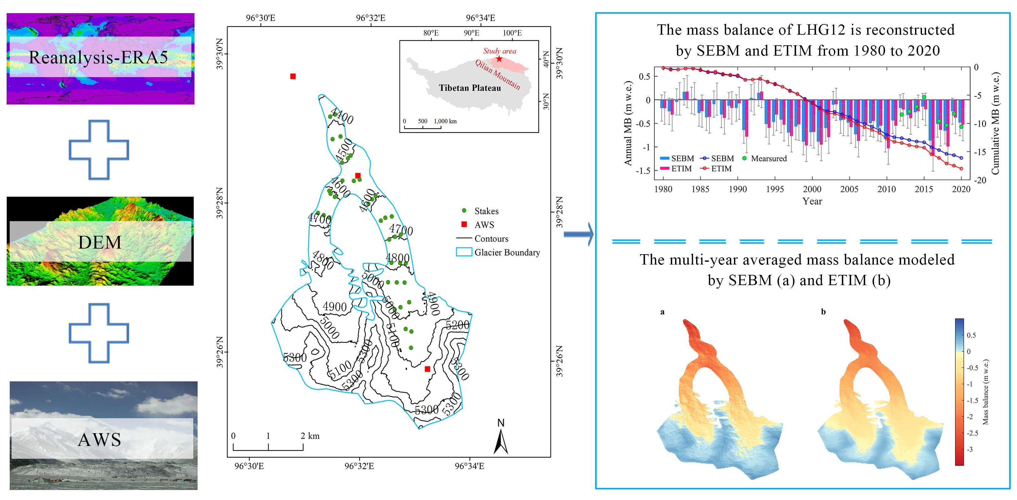
2.1. Study Area
2.2. Data
3. Methods
3.1. Model Description
3.1.1. Simplified Energy Balance Model
3.1.2. Enhanced Temperature-Index Model
3.1.3. Parameterization
3.2. Parameter Calibration and Model Uncertainty
3.3. Model Verification
4. Result
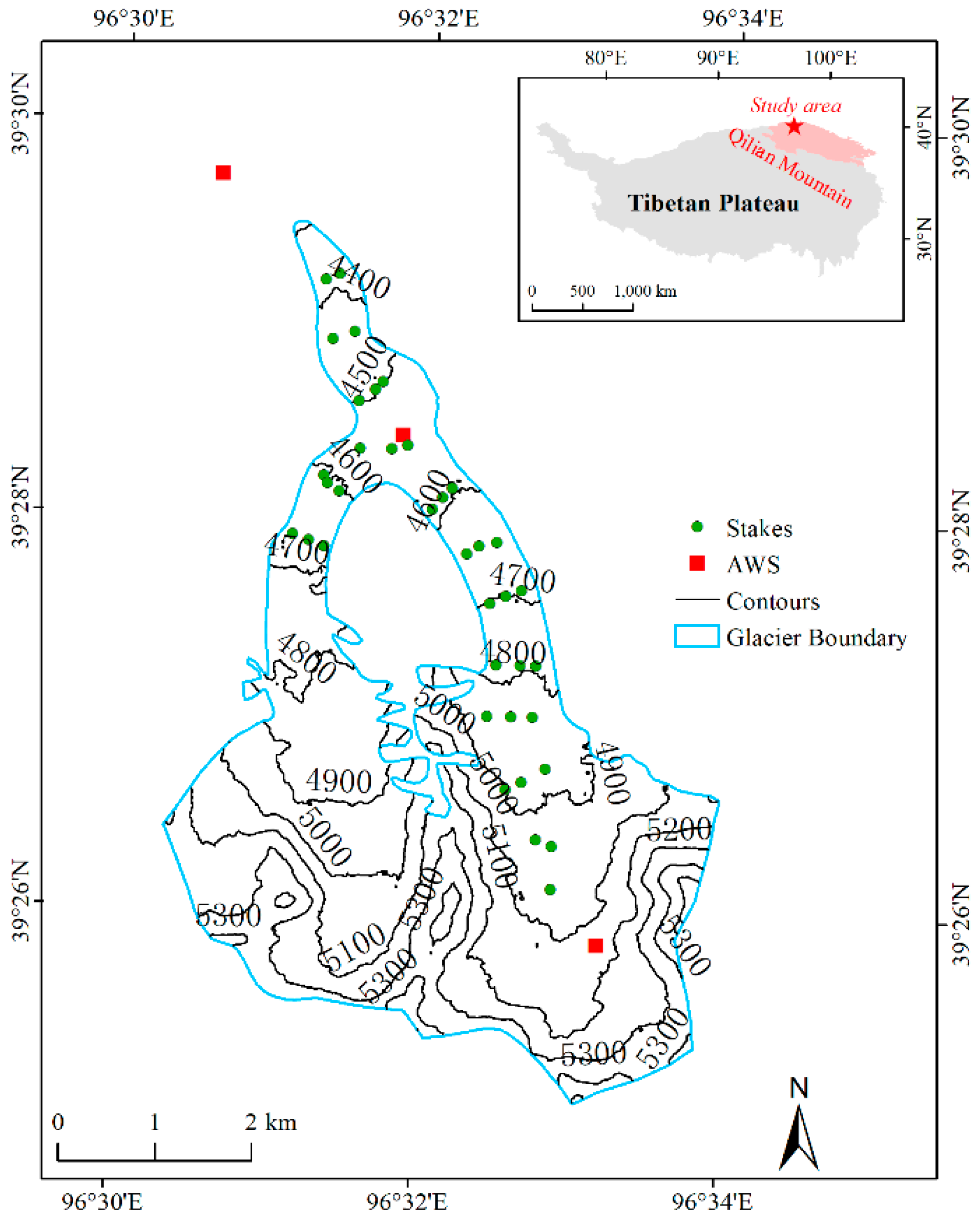
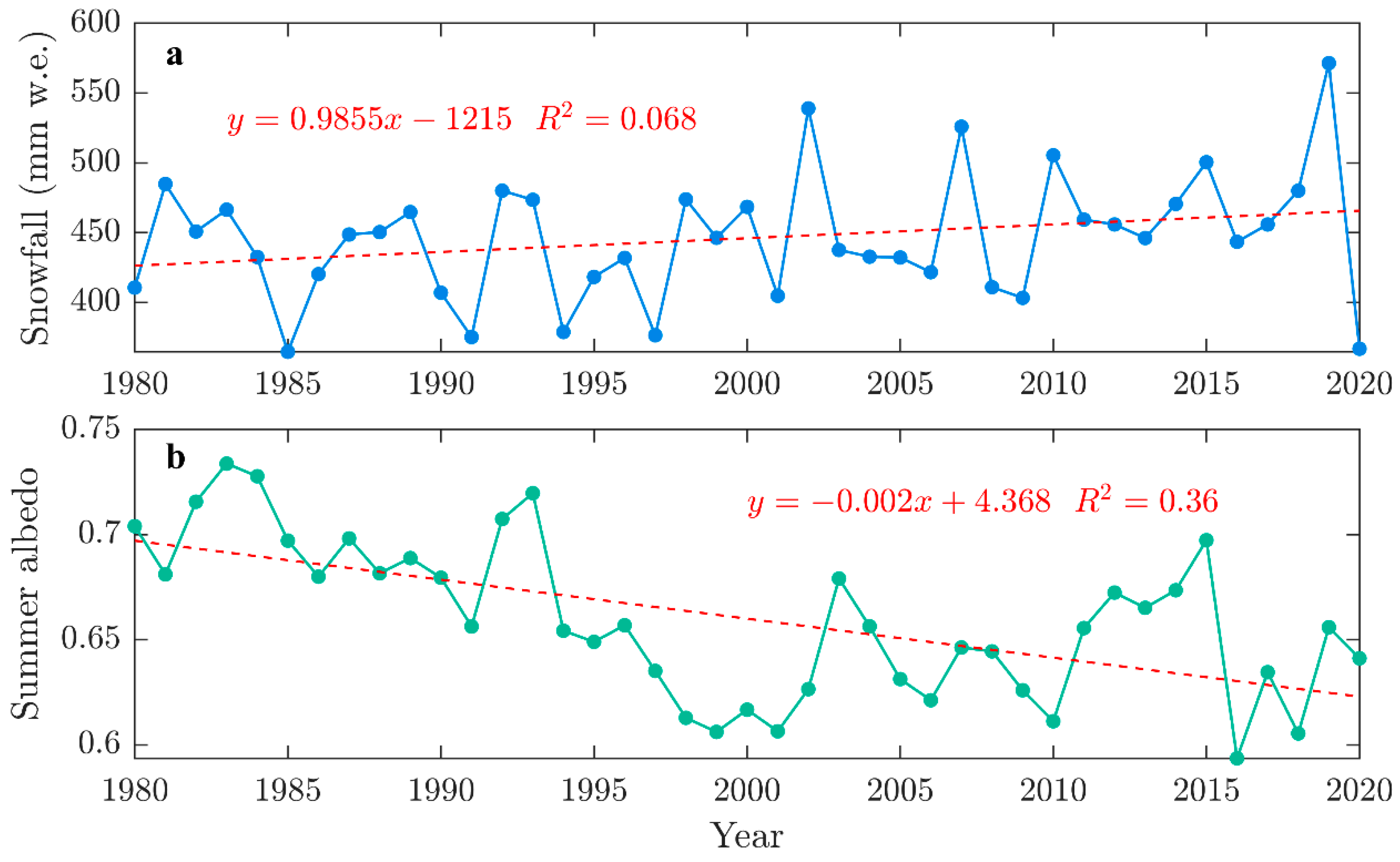
4.1. Meteorological Conditions
4.2. Annual and Cumulative MB
4.3. Seasonal MB
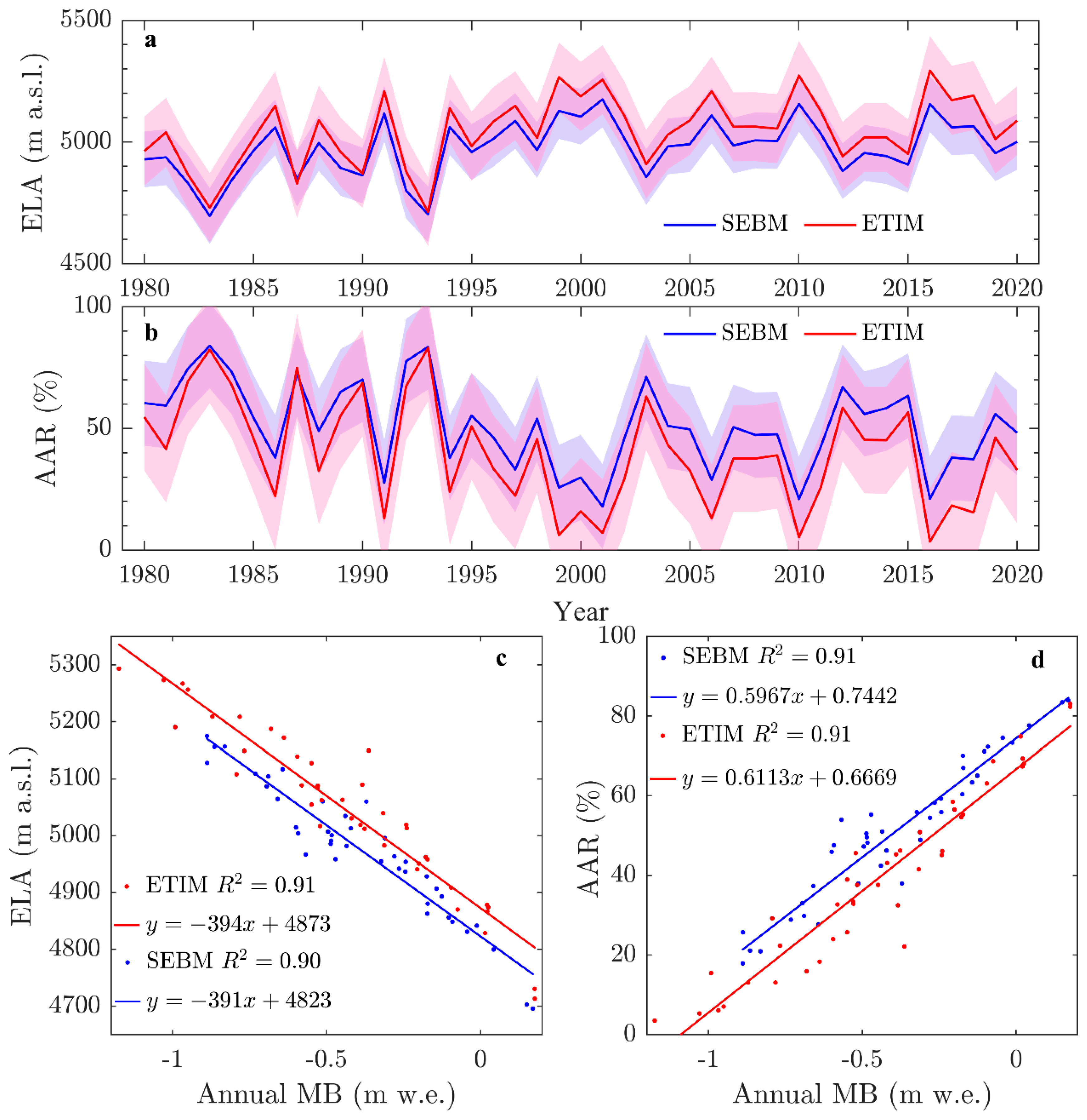
4.4. ELA and AAR
5. Discussion
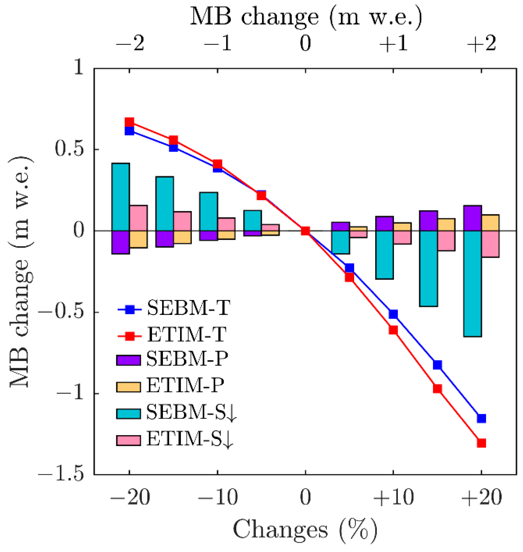
5.1. Response of MB to Climate Change
5.2. Model Differences
6. Conclusions
Author Contributions
Funding
Data Availability Statement
Acknowledgments
Conflicts of Interest
References
- Marzeion, B.; Jarosch, A.H.; Gregory, J.M. Feedbacks and mechanisms affecting the global sensitivity of glaciers to climate change. Cryosphere 2014, 8, 59–71. [Google Scholar] [CrossRef]
- Vuille, M.; Carey, M.; Huggel, C.; Buytaert, W.; Rabatel, A.; Jacobsen, D.; Soruco, A.; Villacis, M.; Yarleque, C.; Elison Timm, O.; et al. Rapid decline of snow and ice in the tropical Andes—Impacts, uncertainties and challenges ahead. Earth Sci. Rev. 2018, 176, 195–213. [Google Scholar] [CrossRef]
- Oerlemans, J. Climate sensitivity of glaciers in southern Norway: Application of an energy-balance model to Nigardsbreen, Hellstugubreen and Alfotbreen. J. Glaciol. 1992, 38, 223–232. [Google Scholar] [CrossRef]
- Oerlemans, J. Glaciers and Climate Change; CRC Press: Boca Raton, FL, USA, 2001. [Google Scholar]
- Deng, H.; Chen, Y.; Li, Y. Glacier and snow variations and their impacts on regional water resources in mountains. J. Geogr. Sci. 2019, 29, 86–102. [Google Scholar] [CrossRef]
- Marzeion, B.; Jarosch, A.; Hofer, M. Past and future sea-level change from the surface mass balance of glaciers. Cryosphere 2012, 6, 1295–1322. [Google Scholar] [CrossRef]
- Yao, T.; Yu, W.; Wu, G.; Xu, B.; Yang, W.; Zhao, H.; Wang, W.; Li, S.; Wang, N.; Li, Z.; et al. Glacier anomalies and relevant disaster risks on the Tibetan Plateau and surroundings. Chin. Sci. Bull. 2019, 64, 2770–2782. [Google Scholar]
- Azam, M.F.; Srivastava, S. Mass balance and runoff modelling of partially debris-covered Dokriani Glacier in monsoon-dominated Himalaya using ERA5 data since 1979. J. Hydrol. 2020, 590, 125432. [Google Scholar] [CrossRef]
- Zhang, Y.; Hirabayashi, Y.; Liu, S. Catchment-scale reconstruction of glacier mass balance using observations and global climate data: Case study of the Hailuogou catchment, south-eastern Tibetan Plateau. J. Hydrol. 2012, 444–445, 146–160. [Google Scholar] [CrossRef]
- Zheng, Z.; Hong, S.; Deng, H.; Li, Z.; Jin, S.; Chen, X.; Gao, L.; Chen, Y.; Liu, M.; Luo, P. Impact of Elevation-Dependent Warming on Runoff Changes in the Headwater Region of Urumqi River Basin. Remote Sens. 2022, 14, 1780. [Google Scholar] [CrossRef]
- Narama, C.; Kääb, A.; Duishonakunov, M.; Abdrakhmatov, K. Spatial variability of recent glacier area changes in the Tien Shan Mountains, Central Asia, using Corona (~1970), Landsat (~2000), and ALOS (~2007) satellite data. Glob. Planet. Chang. 2010, 71, 42–54. [Google Scholar] [CrossRef]
- Guo, Z.; Wang, N.; Shen, B.; Gu, Z.; Wu, Y.; Chen, A. Recent Spatiotemporal Trends in Glacier Snowline Altitude at the End of the Melt Season in the Qilian Mountains, China. Remote Sens. 2021, 13, 4935. [Google Scholar] [CrossRef]
- Yao, T.; Thompson, L.; Yang, W.; Yu, W.; Gao, Y.; Guo, X.; Yang, X.; Duan, K.; Zhao, H.; Xu, B.; et al. Different glacier status with atmospheric circulations in Tibetan Plateau and surroundings. Nat. Clim. Chang. 2012, 2, 663–667. [Google Scholar] [CrossRef]
- Sun, M.; Liu, S.; Yao, X.; Guo, W.; Xu, J. Glacier changes in the Qilian Mountains in the past half-century: Based on the revised First and Second Chinese Glacier Inventory. J. Geogr.Sci. 2018, 28, 206–220. [Google Scholar] [CrossRef]
- Zhang, H.; Li, Z.; Zhou, P. Mass balance reconstruction for Shiyi Glacier in the Qilian Mountains, Northeastern Tibetan Plateau, and its climatic drivers. Clim. Dyn. 2020, 56, 969–984. [Google Scholar] [CrossRef]
- Wang, S.; Yao, T.; Tian, L.; Pu, J. Glacier mass variation and its effect on surface runoff in the Beida River catchment during 1957–2013. J. Glaciol. 2017, 63, 523–534. [Google Scholar] [CrossRef]
- Wang, L.; Qin, X.; Chen, J.; Zhang, D.; Liu, Y.; Li, Y.; Jin, Z. Reconstruction of the glacier mass balance in the Qilian Mountains from 1961 to 2013. Arid Zone Res. 2021, 38, 1524–1533. [Google Scholar]
- Liu, Y.; Qin, D.; Jin, Z.; Li, Y.; Xue, L.; Qin, X. Dynamic Monitoring of Laohugou Glacier No. 12 with a Drone, West Qilian Mountains, West China. Remote Sens. 2022, 14, 3315. [Google Scholar] [CrossRef]
- Pan, B.; Cao, B.; Wang, J.; Zhang, G.; Zhang, C.; Hu, Z.; Huang, B. Glacier variations in response to climate change from 1972 to 2007 in the western Lenglongling mountains, northeastern Tibetan Plateau. J. Glaciol. 2012, 58, 879–888. [Google Scholar] [CrossRef]
- Cao, B.; Guan, W.; Li, K.; Pan, B.; Sun, X. High-resolution monitoring of glacier mass balance and dynamics with unmanned aerial vehicles on the Ningchan No. 1 Glacier in the Qilian Mountains, China. Remote Sens. 2021, 13, 2735. [Google Scholar] [CrossRef]
- Ding, M.; Yang, D.; Broeke, M.R.; Allison, I.; Xiao, C.; Qin, D.; Huai, B. The Surface Energy Balance at Panda 1 Station, Princess Elizabeth Land: A Typical Katabatic Wind Region in East Antarctica. J. Geophys. Res. Atmos. 2020, 125, e2019JD030378. [Google Scholar] [CrossRef]
- Huai, B.; van den Broeke, M.R.; Reijmer, C.H. Long-term surface energy balance of the western Greenland Ice Sheet and the role of large-scale circulation variability. Cryosphere 2020, 14, 4181–4199. [Google Scholar] [CrossRef]
- Jiang, X.; Wang, N.; He, J.; Wu, X.; Song, G. A distributed surface energy and mass balance model and its application to a mountain glacier in China. Chin. Sci. Bull. 2010, 55, 1757–1765. [Google Scholar] [CrossRef]
- Li, H. Spatial and temporal transferability of Degree-Day Model and Simplified Energy Balance Model: A case study. Sci. Cold Arid Reg. 2020, 12, 95–103. [Google Scholar]
- MacDougall, A.; Wheler, B.; Flowers, G. A preliminary assessment of glacier melt-model parameter sensitivity and transferability in a dry subarctic environment. Cryosphere 2011, 5, 1011–1028. [Google Scholar] [CrossRef]
- Linsbauer, A.; Paul, F.; Machguth, H.; Haeberli, W. Comparing three different methods to model scenarios of future glacier change in the Swiss Alps. Ann. Glaciol. 2017, 54, 241–253. [Google Scholar] [CrossRef]
- Azam, M.F.; Wagnon, P.; Vincent, C.; Ramanathan, A.; Linda, A.; Singh, V.B. Reconstruction of the annual mass balance of Chhota Shigri glacier, Western Himalaya, India, since 1969. Ann. Glaciol. 2014, 55, 69–80. [Google Scholar] [CrossRef]
- Zhang, H.; Li, Z.; Zhou, P.; Zhu, X.; Wang, L.I.N. Mass-balance observations and reconstruction for Haxilegen Glacier No.51, eastern Tien Shan, from 1999 to 2015. J. Glaciol. 2018, 64, 689–699. [Google Scholar] [CrossRef]
- Cazorzi, F.; Dalla Fontana, G. Snowmelt modelling by combining air temperature and a distributed radiation index. J. Hydrol. 1996, 181, 169–187. [Google Scholar] [CrossRef]
- Hock, R. A distributed temperature-index ice-and snowmelt model including potential direct solar radiation. J. Glaciol. 1999, 45, 101–111. [Google Scholar] [CrossRef]
- Pellicciotti, F.; Brock, B.; Strasser, U.; Burlando, P.; Funk, M.; Corripio, J. An enhanced temperature-index glacier melt model including the shortwave radiation balance: Development and testing for Haut Glacier d’Arolla, Switzerland. J. Glaciol. 2005, 51, 573–587. [Google Scholar] [CrossRef]
- Jonsell, U.Y.; Navarro, F.J.; Bañón, M.; Lapazaran, J.J.; Otero, J. Sensitivity of a distributed temperature-radiation index melt model based on AWS observations and surface energy balance fluxes, Hurd Peninsula glaciers, Livingston Island, Antarctica. Cryosphere 2012, 6, 539–552. [Google Scholar] [CrossRef]
- Gabbi, J.; Carenzo, M.; Pellicciotti, F.; Bauder, A.; Funk, M. A comparison of empirical and physically based glacier surface melt models for long-term simulations of glacier response. J. Glaciol. 2014, 60, 1140–1154. [Google Scholar] [CrossRef]
- Du, W.; Qin, X.; Liu, Y.; Wang, X. Variation of the Laohugou Glacier No.12 in the Qilian Mountains. J. Glaciol. Geocryol. 2008, 30, 373–379. [Google Scholar]
- Chen, J.; Qin, X.; Kang, S.; Du, W.; Sun, W.; Liu, Y. Potential Effect of Black Carbon on Glacier Mass Balance during the Past 55 Years of Laohugou Glacier No. 12, Western Qilian Mountains. J. Earth Sci. 2020, 31, 410–418. [Google Scholar] [CrossRef]
- Liu, Y.; Qin, X.; Chen, J.; Li, Z.; Wang, J.; Du, W.; Guo, W. Variations of Laohugou Glacier No. 12 in the western Qilian Mountains, China, from 1957 to 2015. J. Mt. Sci. 2018, 15, 25–32. [Google Scholar] [CrossRef]
- Zou, X.; Sun, W.; Yang, D.; Wang, Y.; Li, Y.; Jin, Z.; Du, W.; Qin, X. Effect of cloud on surface energy balance of Laohugou Glacier No.12, Qilian Mountains. J. Glaciol. Geocryol. 2022, 43, 342–356. [Google Scholar]
- Sun, W.; Qin, X.; Du, W.; Liu, W.; Liu, Y.; Zhang, T.; Xu, Y.; Zhao, Q.; Wu, J.; Ren, J. Ablation modeling and surface energy budget in the ablation zone of Laohugou glacier No. 12, western Qilian mountains, China. Ann. Glaciol. 2014, 55, 111–120. [Google Scholar] [CrossRef]
- Wang, L. Simulation and reconstruction of glaciers mass balance in Qilian Mountains from 1961 to 2013. Ph.D. Thesis, University of Chinese Academy of Sciences, Beijing, China, 2022. [Google Scholar]
- Huai, B.; Wang, J.; Sun, W.; Wang, Y.; Zhang, W. Evaluation of the near-surface climate of the recent global atmospheric reanalysis for Qilian Mountains, Qinghai-Tibet Plateau. Atmos. Res. 2021, 250, 105401. [Google Scholar] [CrossRef]
- Wang, Y.; Sun, W.; Wang, L.; Li, Y.; Du, W.; Chen, J.; Qin, X. How do different reanalysis radiation datasets perform in west Qilian Mountains? Front. Earth Sci. 2022, 10, 241. [Google Scholar] [CrossRef]
- Chen, J.; Kang, S.; Qin, X.; Du, W.; Sun, W.; Liu, Y. The mass-balance characteristics and sensitivities to climate variables of Laohugou Glacier No. 12, western Qilian Mountains, China. Sci. Cold Arid Reg. 2017, 9, 543–553. [Google Scholar]
- Jin, Z.; Qin, X.; Sun, W.; Chen, J.; Zhang, X.; Liu, Y.; Li, Y. Monthly variations of temperature gradient in glacierized and non-glacierized areas of the western Qilian Mountains. J. Glaciol. Geocryol. 2019, 41, 282–292. [Google Scholar]
- Huintjes, E.; Sauter, T.; Schroeter, B.; Maussion, F.; Yang, W.; Kropacek, J.; Buchroithner, M.; Scherer, D.; Kang, S.; Schneider, C. Evaluation of a coupled snow and energy balance model for Zhadang glacier, Tibetan Plateau, using glaciological measurements and time-lapse photography. Arc. Antarct. Alp. Res. 2015, 47, 573–590. [Google Scholar] [CrossRef]
- Kang, E.; Cheng, G.; Lan, Y.; Jin, H. A model for simulating the response of runoff from the mountainous watersheds of inland river basins in the arid area of northwest China to climatic changes. Sci. China Ser. D Earth Sci. 1999, 42, 52–63. [Google Scholar] [CrossRef]
- Sun, W.; Qin, X.; Ren, J.; Wu, J.; Du, W.; Liu, Y.; Hou, D. Surface Energy Balance in the Accumulation Zone of the Laohugou Glacier No.12 in the Qilian Mountains during Ablation Period. J. Glaciol. Geocryol. 2011, 33, 38–46. [Google Scholar]
- Oke, T.R. Boundary Layer Climates; Routledge: London, UK, 2002. [Google Scholar]
- Hock, R. Glacier melt: A review of processes and their modelling. Prog. Phys. Geogr. Earth Environ. 2005, 29, 362–391. [Google Scholar] [CrossRef]
- Brock, B.W.; Willis, I.C.; Sharp, M.J. Measurement and parameterization of albedo variations at Haut Glacier d’Arolla, Switzerland. J. Glaciol. 2000, 46, 675–688. [Google Scholar] [CrossRef]
- Jiang, X.; Wang, N.; He, J.; Song, G.; Yang, S.; Wu, X. A Study of Parameterization of Albedo on the Qiyi Glacier in Qilian Mountains, China. J. Glaciol. Geocryol. 2011, 33, 30–37. [Google Scholar]
- Gao, L.; Hao, L.; Chen, X. Evaluation of ERA-interim monthly temperature data over the Tibetan Plateau. J. Mt. Sci. 2014, 11, 1154–1168. [Google Scholar] [CrossRef]
- Zhao, D.; Gao, X.; Wu, S.; Zheng, D. Trend of Climate Variation in China from 1960 to 2018 Based on Natural Regionalization. Adv. Earth Sc. 2020, 35, 750–760. [Google Scholar]
- Liu, Y.; Qin, D.; Li, Y.; Qin, X.; Li, Z.; Wang, J.; Jin, Z.; Wang, L. Changes in the Surface Elevation of the Laohugou Glacier No. 12 in Western Qilian Mountains. Front. Earth Sci. 2022, 10, 832701. [Google Scholar] [CrossRef]
- Ohmura, A. Changes in mountain glaciers and ice caps during the 20th century. Ann. Glaciol. 2017, 43, 361–368. [Google Scholar] [CrossRef]
- Yang, W.; Yao, T.; Guo, X.; Zhu, M.; Li, S.; Kattel, D.B. Mass balance of a maritime glacier on the southeast Tibetan Plateau and its climatic sensitivity. J. Geophys. Res. Atmos. 2013, 118, 9579–9594. [Google Scholar] [CrossRef]
- Wang, S.; Pu, J.; Wang, N. Study of Mass Balance And Sensibility to Climate Change of Qiyi Glacier in Qilian Mountains. J. Glaciol. Geocryol. 2011, 33, 1214–1221. [Google Scholar]


| Parameters | Unit | Value Used in Model | Change for Model Uncertainty | |
|---|---|---|---|---|
| Albedo | - | −0.0266 | ±25% | |
| - | 0.6785 | ±25% | ||
| - | −0.0942 | ±25% | ||
| - | −0.1371 | ±25% | ||
| - | 0.3594 | ±25% | ||
| - | −0.0316 | ±25% | ||
| mm | 5 | ±25% | ||
| Precipitation separation | °C | 2 | 1.5~2.5 | |
| °C | −2 | −2.5~−1.5 | ||
| SEBM | W m−2 °C−1 | 9 | 8~10 | |
| W m−2 | −68 | −70~−65 | ||
| ETIM | mm d−1 °C−1 | 3.6 | 3.2~4 | |
| mm m2 d−1 W−1 | 0.176 | 0.17~0.18 | ||
Publisher’s Note: MDPI stays neutral with regard to jurisdictional claims in published maps and institutional affiliations. |
© 2022 by the authors. Licensee MDPI, Basel, Switzerland. This article is an open access article distributed under the terms and conditions of the Creative Commons Attribution (CC BY) license (https://creativecommons.org/licenses/by/4.0/).
Share and Cite
Wu, J.; Sun, W.; Huai, B.; Ding, M.; Wang, L.; Wang, Y.; Zhang, J.; Du, W.; Chen, J.; Qin, X. Mass Balance Reconstruction for Laohugou Glacier No. 12 from 1980 to 2020, Western Qilian Mountains, China. Remote Sens. 2022, 14, 5424. https://doi.org/10.3390/rs14215424
Wu J, Sun W, Huai B, Ding M, Wang L, Wang Y, Zhang J, Du W, Chen J, Qin X. Mass Balance Reconstruction for Laohugou Glacier No. 12 from 1980 to 2020, Western Qilian Mountains, China. Remote Sensing. 2022; 14(21):5424. https://doi.org/10.3390/rs14215424
Chicago/Turabian StyleWu, Jiake, Weijun Sun, Baojuan Huai, Minghu Ding, Lei Wang, Yuzhe Wang, Junlong Zhang, Wentao Du, Jizu Chen, and Xiang Qin. 2022. "Mass Balance Reconstruction for Laohugou Glacier No. 12 from 1980 to 2020, Western Qilian Mountains, China" Remote Sensing 14, no. 21: 5424. https://doi.org/10.3390/rs14215424
APA StyleWu, J., Sun, W., Huai, B., Ding, M., Wang, L., Wang, Y., Zhang, J., Du, W., Chen, J., & Qin, X. (2022). Mass Balance Reconstruction for Laohugou Glacier No. 12 from 1980 to 2020, Western Qilian Mountains, China. Remote Sensing, 14(21), 5424. https://doi.org/10.3390/rs14215424