JPSS-1 VIIRS Prelaunch Reflective Solar Band Testing and Performance

Abstract

The Visible Infrared Imaging Radiometer Suite (VIIRS) instruments on board both the Suomi National Polar-orbiting Partnership (S-NPP) and the first Joint Polar Satellite System (JPSS-1) spacecraft provides calibrated reflectance, radiance, and brightness temperature products for weather and climate applications. It has 22 bands with resolutions of 375 and 750 m for imaging and moderate bands, respectively, on 4 focal planes covering a spectral range of 400–12,490 nm. The bands are stratified into reflective solar bands (RSBs), thermal emissive bands (TEBs), and the Day/Night Band (DNB). VIIRS has three on-board calibration sectors: the solar diffuser (SD), on-board calibrator blackbody (OBCBB), and space view (SV). The on-board calibrator targets are used to track on-orbit degradation and background offset drift. Extensive prelaunch radiometric testing of the RSB, TEB, and DNB detector’s radiometric sensitivity and noise was performed for both S-NPP and JPSS-1 VIIRS. The combination of prelaunch testing and on-orbit calibrators is used to produce calibrated sensor data record (SDR) reflectance, radiance, and brightness temperatures for use in environmental data record (EDR) products. This paper will discuss the prelaunch radiometric calibration activities for the RSBs only and includes the dynamic range, calibration coefficients, detector noise, and radiometric uncertainties for JPSS-1 VIIRS.

1. Introduction

The first Joint Polar Satellite System (JPSS-1) spacecraft is a follow-on mission of the Suomi National Polar-orbiting Partnership (S-NPP) with a similar sensor suite as its predecessor. The Visible Infrared Imaging Radiometer Suite (VIIRS), on board both S-NPP and JPSS-1, is a cross-track scanning sensor in a sun-synchronous low Earth orbit with an altitude of ~840 km, an equatorial crossing of 13:30 Greenwich Mean Time, and a scan range of ±56.0° covering a swath width of 3060 km [1]. VIIRS uses a rotating telescope assembly (RTA) and a double-sided half-angle mirror (HAM) combination to provide the cross-track scanning. The two HAM sides (HAM A and B) have the same mirror coating design but are slightly different in performance due to different mirror deposition times and must be characterized individually. It has 22 bands covering the 395–12,490 nm spectral region using four different focal plane assemblies (FPAs). The reflective solar bands (RSBs) are on the visible near-infrared (VNIR) focal plane (bands M1–M7 and I1–I2), which covers a spectral range of 395–900 nm, and the short- and midwave infrared (SMIR) FPA (bands M8–M11 and I3), having a spectral range of 1230–2500 nm. The thermal emissive bands (TEBs) are on the SMIR FPA (bands M12, M13, and I4), with a spectral range of 3700–4130 nm, and the long -wave infrared (LWIR) FPA (bands M14–M16 and I5), with a spectral range of 8400–12,490 nm. The fourth FPA contains a single panchromatic high dynamic range Day/Night Band (DNB) covering the 500–900 nm spectral range. There are two spatial resolutions, with the imaging (I1–I5) and moderate (M1–M16 and DNB) resolution bands having a ground footprint of 375 and 750 m, respectively. The non-DNB bands have a cross-track aggregation scheme, due to the Earth’s curvature, to mitigate pixel growth within the swath of the sensor data record (SDR) image. This requires that three samples in the ±32° scan angle region are combined to make a ground pixel, while the −43° to −32° and 32° to 43° scan region combines two samples to make a ground pixel, and the −56° to −43° and 43° to 56° scan region uses a single sample to make a ground pixel. Figure 1 shows the ground pixel growth if there is no aggregation in (green and light blue lines for track and scan, respectively) and the reduced size in ground pixel when the aggregation scheme is implemented in the scan direction (dark blue line). The aggregation along-scan attempts to reduce the pixel growth and maintain a 750 m resolution throughout the scan. There are 32 and 16 detectors for the imaging and moderate bands, respectively, to provide contiguous ground coverage between scans.

Like its heritage sensors, Advanced Very High Resolution Radiometer (AVHRR) [2], Moderate Resolution Imaging Spectroradiometer (MODIS) [3], and Operational Linescan System (OLS) [4], VIIRS provides calibrated top-of-atmosphere (TOA) brightness temperature, radiance, and reflectance products for weather and geoscience applications. The VIIRS band’s environmental data record (EDR) product applications cover a wide range of scene types, from dark/warm oceans to bright/cold clouds [5,6,7,8]. This requires the bands to have a signal-to-noise (SNR) requirement that ensures EDR performance under these differing scene conditions. To achieve the SNR requirements, several VIIRS bands are dual gain. This allows the SNR at low and high radiance scenes to be high while covering a wide dynamic range.

Table 1. VIIRS spectral, dynamic range, and noise requirements for the reflective solar bands.

Band	Spectral Range (µm)	Band Gain	Ltyp	Lmax	SNR
VNIR
DNB	0.500–0.900	VG	0.00003	200	6
M1	0.402–0.422	High	44.9	135	352
		Low	155	615	316
M2	0.436–0.454	High	40	127	380
		Low	146	687	409
M3	0.478–0.498	High	32	107	416
		Low	123	702	414
M4	0.545–0.565	High	21	78	362
		Low	90	667	315
I1	0.600–0.680	Single	22	718	119
M5	0.662–0.682	High	10	59	242
		Low	68	651	360
M6	0.739–0.754	Single	9.6	41	199
I2	0.846–0.885	Single	25	349	150
M7	0.846–0.885	High	6.4	29	215
		Low	33.4	349	340
SWIR
M8	1.230–1.250	Single	5.4	165	74
M9	1.371–1.386	Single	6	77.1	83
I3	1.580–1.640	Single	7.3	72.5	6
M10	1.580–1.640	Single	7.3	71.2	342
M11	2.225–2.275	Single	0.12	31.8	10

lists the dynamic range requirements and the SNR level at a typical scene for each band. RSBs M1–M5 and M7 have high (dark scene radiance) and low (bright scene radiance) gain stages, and the DNB has high, middle, and low gain stages to handle night, terminator, and day scenes, respectively. This requires the radiometric calibration to be characterized for each band’s gain stage, HAM side, and detector.

VIIRS has three internal calibration sectors with the space view (SV) looking into dark space at a dark/cold background reference, the on-board calibrator blackbody (OBCBB) for TEB on-orbit response degradation, and the solar diffuser (SD) for RSB gain degradation [5]. Figure 2 shows a diagram of the VIIRS internal calibration views throughout the VIIRS scan in relation to the Earth view (EV) observation. The RSBs use a two-point calibration (SV offset and SD illumination) to determine the optical system’s linear gain change in Equation (1).

$$F=\left[\frac{\overline{H\left(t,\lambda \right)E\left(\lambda \right){\tau }_{SAS}\left({\varphi }_{dec},{\varphi }_{az},\lambda \right)BRDF\left({\varphi }_{dec},{\varphi }_{az},\lambda \right)}\cos \left({\theta }_{inc}\right)}{c_0+c_{1}d{n}_{SD}+c_{2}d{n}_{SD}^2}\right]$$

(1)

The dnSD is the average of the 96-sample I-band or 48-sample M-band detector response from the SV subtracted from each sample averaged SD response. This removes the instrument’s digital count offset and any dark noise drifts on a scan-by-scan basis. The radiance of the Sun uses an estimation of the solar spectral irradiance E(λ) (λ denotes wavelength) at the location of the satellite, the bidirectional reflectance distribution function (BRDF) of the SD, and the solar attenuation screen transmission τ_SAS [9]. These parameters are dependent on solar azimuth (ϕ_az) and solar declination (ϕ_dec), in the spacecraft coordinate system. θ_inc is solar incidence angle at the SD, defined as the angle between a vector pointing to the Sun and the vector normal to the SD surface. The H factor scales the SD BRDF to account for degradations due to solar UV exposure and is computed using the solar diffuser stability monitor (SDSM) [10]. Figure 3 shows the geometry for the SD and SDSM during H factor data collection. The H factor in Equation (1) is determined using

$$H=\frac{\left(D{C}_{sun}-D{C}_{bkg}\right)}{\left(D{C}_{sd}-D{C}_{bkg}\right)}\cdot \frac{{\tau }_{SAS}({\alpha }_{az},{\beta }_{dec})\cdot BRD{F}_{sd}({\alpha }_{az},{\beta }_{dec})\cdot {\sin }^2(FO{V}_{SDSM})\cdot \cos (AO{I}_{sd})}{{\tau }_{SDSM}({\alpha }_{az},{\beta }_{dec})}$$

(2)

with τ_SDSM (the SDSM screen transmittance) and τ_SAS both being a function of SDSM solar azimuth α_az and declination β_dec angles. The DC_sun, DC_sd, and DC_bkg values are the detector voltage from the Sun, SD, and background paths, respectively, as measured by the SDSM internal detectors. FOV_SDSM is the fixed field of view of the SDSM when looking at the SD, AOI_sd is the angle of incidence of the SDSM view relative to the SD’s normal vector, and BRDF_sd is the SD reflectance at the SDSM view geometry.

The Earth view radiance (L_EV) is retrieved using the F factor, prelaunch calibration coefficients, response versus scan angle (RVS), and dn_EV (the SV subtracted Earth view response), as shown in Equation (3) [11].

$$L_{EV}=F\frac{RVS\left({\theta }_{SD}\right)}{RVS\left({\theta }_{EV}\right)}\left(a_0+a_{1}d{n}_{EV}+a_{2}d{n}_{EV}^2+a_{3}d{n}_{EV}^3\right)$$

(3)

The RVS captures HAM mirror reflectance changes during the scan, and scales the calibration coefficients (c_i) accordingly, to compensate for this gain variation between the RVS_EV and RVS_SD scan angles [12]. The RVS curve is a function of scan angle and is characterized during prelaunch testing. The calibration coefficients (c_i) can have up to a third-order polynomial in the on-orbit SDR algorithm. The JPSS-1 VIIRS instrument uses a second polynomial fit for the VNIR bands and a third-order term for the SWIR bands.

The dns and DC values in Equations (1)–(3) are determined using digital response of the VIIRS or SDSM detectors and are real time in situ measurements of the light within the sensor. The calibration coefficients ci are used to convert these counts into a calibrated radiance using Equations (1)–(3). These calibration coefficients are determined through extensive prelaunch characterization using National Institute of Standards and Technology (NIST) traceable radiance sources. The next section will describe the test and data analysis methodologies used to characterize the calibration coefficients and the sensor requirements used to evaluate their performance.

The SD BRDF, attenuator screens in the SD and SDSM, and geometry factors for Equations (1) and (2) are determined before launch with component level measurements of each system. The screen transmittance and SD BRDF are measured at multiple azimuth and declination angles to characterize the angular dependence of their transmission and reflectance, respectively. The geometric factors used in the calibration are modeled based on specified build sizes and alignment measurements, acquired during component level integration. The solar irradiance is Thuillier 2003 and considered to be a fixed intensity throughout the on-orbit mission [13]. The solar irradiance used for S-NPP and JPSS-1 SDR processing is different [14]. This results in radiance differences between sensor SDRs, but the reflectance product is not affected. Prelaunch measurements to characterize the RVS are not discussed in this paper but are detailed in [12]. These prelaunch values used for estimating the solar radiance are covered in more detail in the uncertainty section, where an error tree of the values is rolled up into a full-system-level radiometric uncertainty.

The last part of this paper is the measurement of the detector noise and SNR. Prelaunch measurements were taken, at sensor-level TVAC in the summer of 2014, and spacecraft testing in early 2015, to look at the dark, pattern, frequency, and shot noise features for each detector. The test methodology, analysis approaches, and performance will be discussed for sensor-level TVAC testing. These results are also rolled up into the RSB radiometric uncertainty analysis for each along-scan aggregation zone.

2. RSB Calibration Testing Approach

2.1. Spherical Integration Source and Linear Attenuation Assembly Calibrators

The RSBs’ wide spectral diversity, dynamic range, and detector field of view require a unique source to radiometrically calibrate the sensor. A spherical integration source with a 100 cm diameter (SIS100) that provides a spatially uniform, unpolarized wide field of view target is used to calibrate all the RSBs (excluding bands M1–M3 low gains). A small high-brightness SIS mounted on the three-mirror collimator (TMCSIS) source is used to calibrate bands M1–M3 low gain, since SIS100 cannot cover the top of their dynamic range. Figure 4 shows the layout of the SIS100, TMCSIS, and SV source with respect to the VIIRS sensor in the TVAC chamber.

SIS100 has 18, 9, and 10,200 W, 45 W, and 8 W bulbs, respectively, that provide a wide range of illumination levels for each band. The internal cavity of SIS100 is coated with a diffuse material that scatters the lamp illumination within the sphere to produce a uniform illumination field at the exit aperture of the sphere. The SIS100 lamp filaments have a brightness temperature profile that emits more energy in the NIR region as compared with the on-orbit solar brightness temperature shown in Figure 5. The differences in brightness temperatures between the ground and on-orbit sources will cause errors in the sensor calibration due to out-of-band (OOB) relative spectral response (RSR) contributions. This is captured as an uncertainty in the prelaunch radiometric calibration coefficients when used on orbit and is included in the uncertainty analysis discussed in Section 3.

SIS100 is calibrated using a NIST traceable ASD spectrometer for each lamp configuration used for the test. The uncertainty of the calibrated radiance during 1–5% is larger than that required to meet the prelaunch calibration coefficient uncertainty requirement of 0.3%. To mitigate this issue, a linear attenuator assembly (LAA) was designed to provide a differential characterization approach that allows the shape of the detector response to be characterized independent of the SIS100 radiance. Equation (4) is the attenuator methodology for characterizing the detector shape:

$$L_{SIS100}=c_0+c_{1}d{n}_{out}+c_{2}d{n}_{out}^2$$

(4)

The $d{n}_{out}$ corresponds to the VIIRS response when viewing SIS100 with the LAA out of the optical path, $d{n}_{in}$ when the LAA attenuates the SIS100 radiance in the VIIRS optical path, τ is the transmission of the LAA, and $\frac{c_0}{c_1}$ and $\frac{c_2}{c_1}$ are the ratio of the offset and nonlinear terms (c₀ and c₂) normalized by the linear component ($c_1$) of the second-order polynomial. The dn is the difference between the DNs when viewing the SIS minus the DNs from the SV sector. A deep cavity blackbody cooled to ~95 K is used to provide a deep space equivalent source for the SV sector and provides a background DN offset correction. The response characterization uncertainty using Equation (4) is evaluated relative to the sensor requirement to determine whether a higher-order polynomial fit is necessary. For JPSS-1 VIIRS, a second-order fit provided the fit performance to meet the characterization requirements. A value of $d{n}_{in}$ and $d{n}_{out}$ for each SIS100 source level that is measured, by the sensor, is used in a least squares regression to determine the τ, $\frac{c_0}{c_1}$, and $\frac{c_2}{c_1}$ values for each band, detector, subframe, HAM side, and gain state. Equation (5) uses a single SIS100 calibrated radiance (L_SIS100) value coupled with its corresponding $d{n}_{out}$ to determine the $c_1$ calibration coefficient.

$$L_{SIS100}=\frac{\left(c_0+c_{1}d{n}_{in}+c_{2}d{n}_{in}^2\right)}{{\tau }_{LAA}}$$

(5)

Setting Equations (4) and (5) equal to remove the radiance of the SIS100 (L_SIS100) term and rearranging the terms allows the shape of the detector response relative to the linear terms $\frac{c_0}{c_1}$ and $\frac{c_2}{c_1}$ to be determined with the other fit parameter, the LAA transmittance ${\tau }_{LAA}$.

$$d{n}_{in}=\left({\tau }_{LAA}-1\right)\frac{c_0}{c_1}+{\tau }_{LAA}d{n}_{out}+\frac{c_2}{c_1}\left({\tau }_{LAA}d{n}_{out}^2-d{n}_{in}^2\right)$$

(6)

This removes the uncertainties due to SIS100 radiance knowledge from the characterization of the detector response shape. It also reduces the impact of SIS100 source drifting during a 30 h test if Equation (6) is used to characterize the calibration coefficients. The collection of $d{n}_{out}$ and $d{n}_{in}$ set for a single SIS100 level is in the order of ~10 min and reduces the impacts of SIS100 drifting during the characterization. The $d{n}_{out}$ and $d{n}_{in}$ parameters are a function of the band, detector, HAM side, gain, and subsample (for I-bands only) for each SIS100 lamp level measured during the test. A least squares regression using Equation (6) with ${\tau }_{LAA}$, $\frac{c_0}{c_1}$, and $\frac{c_2}{c_1}$ as fit parameters is performed to find the detector calibration coefficients relative to the linear term. Equation (6) can be rearranged to solve for $c_1$ and is used to get the linear term in Equation (7).

$$c_1=\frac{L_{SIS100}}{\left(\frac{c_0}{c_1}+d{n}_{out}+\frac{c_2}{c_1}d{n}_{out}^2\right)}$$

(7)

The $c_1$ term uses the detector response shape coefficients from Equation (6) least squares regression, the $d{n}_{out}$ from a SIS100 level, and the SIS100 radiance after monitor correction to estimate the linear response coefficient. The selection of the SIS100 radiance level will determine the source calibration bias in the calibration coefficients. The ${\tau }_{LAA}$, $\frac{c_0}{c_1}$, and $\frac{c_2}{c_1}$ can also be fixed to a constant value, for example, $\frac{c_0}{c_1}$ set equal to zero, during the regression fit using Equation (6). This allows test setup errors to be reduced in the derived prelaunch calibration coefficients. This $c_1$ is multiplied into the $\frac{c_0}{c_1}$ and $\frac{c_2}{c_1}$ to derive the calibration coefficients used on orbit in Equations (1) and (3). The radiance of SIS100 (L_SIS) is adjusted for lamp degradation during the thermal vacuum (TVAC) test phase by the use of a radiance stability monitor mounted on SIS100. The stability monitor measures the VNIR radiance output of SIS100 simultaneously with the VIIRS characterization measurements to adjust the radiance using in situ measurements.

The TMCSIS uses a three-mirror collimator to image the exit aperture of a high-brightness SIS onto the full field of the VIIRS VNIR FPA detectors and provides higher radiance illumination to VIIRS than SIS100. A smaller TMCSIS with collimator mirror angular reflectance variation results in a more non-uniform illumination at the VIIRS detectors than that observed with SIS100. A single bulb inside the TMCSIS provides the illumination source, and its input current is varied to adjust the intensity level. This allows multiple M1–M3 low gain response levels to be measured throughout its dynamic range. Like the SIS100 test setup, the TMCSIS uses the LAA to measure the difference in detector response between in and out configurations. This reduces the impact of the TMCSIS spatial non-uniformity and the temporal changes in the lamp’s irradiance. The TMCSIS does not have a radiance monitor and therefore, calibration coefficients derived from this source rely on a cross-calibration with SIS100.

2.2. JPSS-1 VIIRS Configuration and Test Plan

The radiometric response characterization and noise performance are measured in TVAC for the RSBs. The test plan includes SIS measurements at three temperature plateaus: cold (−20 °C), nominal (−5 °C), and hot (10 °C) performance and on both the primary and redundant electronic sides. Measurements at a fixed SIS100 lamp level are also taken during the transition between cold-to-nominal and nominal-to-hot plateaus. This allows the temperature sensitivity of the sensor to be characterized outside of the three steady-state plateaus for on-orbit gain compensation purposes. A pair of temperature and humidity monitors, one on SIS100 and one on the TVAC chamber window, are used to adjust the radiance for water vapor absorption effects for band M9 only.

At each temperature plateau and electronics side, the radiometric characterization test utilizes over 40 individual SIS100 lamp levels to allow the characterization of all the bands (excluding M1–M3 LG) through their dynamic range. Each lamp level has three unique VIIRS sensor configurations, fixed high gain, fixed low gain, and auto gain, with each of these configurations taking two measurements of the LAA in and out of the optical path. This allows the band’s high and low gain measurements to be acquired near simultaneously in time and have the response in the on-orbit auto gain configuration to be captured for comparison with its fixed counterparts. These measurements are acquired in an LAA out, in, in, out pattern to reduce the impact of small source drifts during the data collections. The dual gain switching for bands M1–M5 and M7 is also evaluated using the auto gain measurements by looking for SIS100 levels where the band’s response has both gain states within its collection.

The TMCSIS measurements, for response characterization of bands M1–M3 LG, utilizes 13 unique radiance levels by adjusting the current on the source’s bulb. The collection methodology differs with respect to the SIS100 collections in that there are no high or auto gain measurements during the response characterization portion of the test. There is, however, a cross-calibration portion of this test phase, where both high and low gain measurements of the TMCSIS and SIS100 are collected to transfer the SIS100 calibration to the TMCSIS. This is performed by adjusting the TMCSIS’s lamp current so that the VIIRS response closely matches the response from a given SIS100 lamp level. This response matching is performed for each of the three bands in unique collections, and the cross-calibration is discussed in the next section.

During the transitions between the performance plateaus, SIS100 is fixed at one lamp level, and the sensor’s integration time is varied to measure fixed high gain responses within the band’s dynamic range with high SNRs. The temperature sensitivity of the RSB response is believed to be due to electronics module (EM) and FPA temperature effects. Therefore, during the performance plateau transitions, the EM and FPA are elevated in temperature at different times. This allows the separation of their temperature sensitivities in the measured detector response.

2.3. Test Data and Analysis Methodology

The RSB radiometric testing covers response characterization, dynamic range verification, SNR at Ltyp, dual gain transition determination, and temperature-dependent gain sensitivity. The methodology for the determination of each of these metrics will be discussed in this section. The radiometric uncertainty calculations and error budget metrics will be discussed in the next section.

The dynamic range analysis uses a digital number (DN) average of approximately 100 M-band samples and 50 scans when viewing SIS100 with the DC offset subtracted using the SV sector DNs to get what is called dn. This dn is computed for each band, detector, HAM side, gain (using fixed high or low), and subsample (for I-bands only) for all SIS100 lamp levels. A linear fit of SIS100 radiance (corrected using the radiance monitor) with dns is performed using unsaturated offset corrected detector response data. The maximum unsaturated dn response of the detector is then used in the linear fit to assess the maximum measurable radiance. This value is then compared with the specification in Table 1 to determine compliance.

The SNR is computed using the same data as the dynamic range calculation. Equation (8) is the SNR computation for the VIIRS detectors.

$$SNR=\langle {\frac{\langle dn{\left(Sample\right)\rangle }_{scan}}{\langle {\left(Sample\right)\rangle }_{scan}}\rangle }_{sample}$$

(8)

The dns are averaged over the 50 scans for each of the approximated 100 M-band samples with the standard deviation (σ) also computed. The ratio of the dns to σ is the SNR and is computed for each band, detector, HAM side, gain and subframe (I-bands only), SIS100 level, and sample. The SNRs are then averaged over samples to derive the final value. This average response over scan and then SNR over sample is to reduce the impact of the SIS100 spatial non-uniformity on the σ values. The SNR versus SIS100 radiance is modeled with

$$SNR=\frac{L_{SIS100}}{\sqrt{a_0+a_1{L}_{SIS100}+a_2{L}_{SIS100}^2}}$$

(9)

where the a coefficients model the dark, read, and shot noise of the detector. This fit is then used to compute the SNR at the band’s specified Ltyp for each detector, HAM side, gain, and subsample (for I-bands only).

The dual gain switch point analysis uses the auto gain portion of the SIS100 test to evaluate the transition from high to low gains. The analysis looks at the detector response, while the detector scans across the SIS100 exit port. This provides samples with varying amounts of SIS100 illumination within the field of view of the detector. As the instrument scans across the SIS100 exit port, the detector response increases through the high gain dynamic range until the SIS100 signal fills enough of the detector’s field of view to cause a gain transition. The signal at that sample where the transition occurs is used to determine the detector’s gain switch point.

The response characterization of the RSBs has two parts: the first is characterizing the response shape using the LAA approach and then using a SIS100 radiance level to tie the response shape to a calibrated radiance scale. A polynomial fit, shown in Equation (4), is used to model the detector’s response versus SIS100 radiance with ci corresponding to the detector calibration coefficients and $d{n}_{out}$ the detector response at each SIS100 radiance level with no LAA in the path. The response with the LAA in the optical path is modelled using Equation (5) with ${\tau }_{LAA}$ corresponding to the transmission of the LAA pinhole screen and $d{n}_{in}$ representing the detector response when viewing SIS100 with LAA attenuation. The SIS100 radiance level selection and regression approach will be discussed in the next section.

3. Results

3.1. Dynamic Range

The dynamic range for JPSS-1 VIIRS, shown in

Table 2. Measured dynamic range performance for the reflective solar bands. Bands I3 and M8 fail the sensor specification, and band M9 shows just below the requirements but has impacts of water absorption in the analysis and most likely passes the requirements.

	Single Gain			High Gain			Low Gain
	L_sat	L_max	L_sat/L_max	L_sat	L_max	L_sat/L_max	L_sat	L_max	L_sat/L_max
I1	772	718	1.08	--	--	--	--	--	--
I2	401	349	1.15	--	--	--	--	--	--
I3	65.2	72.5	0.90	--	--	--	--	--	--
M1	--	--	--	164	135	1.21	710	615	1.15
M2	--	--	--	173	127	1.36	797	687	1.16
M3	--	--	--	144	107	1.35	851	702	1.21
M4	--	--	--	113	78.0	1.44	863	667	1.29
M5	--	--	--	76.5	59.0	1.30	733	651	1.13
M6	46.8	41.0	1.14	--	--	--	--	--	--
M7	--	--	--	38.1	29.0	1.31	414	349	1.19
M8	115	165	0.69	--	--	--	--	--	--
M9	72.1	77.1	0.93	--	--	--	--	--	--
M10	77.0	71.2	1.08	--	--	--	--	--	--
M11	33.5	31.8	1.05	--	--	--	--	--	--

, meets or exceeds the requirements listed in Table 1 for all bands except M8 and I3 and is comparable in performance to S-NPP VIIRS [15]. Figure 6 shows an example of the dynamic range for band M4 in auto gain for HAM B. The vertical red lines correspond to the Lmax for high (left) and low (right) gain, respectively, and the points show how each detector’s response (y-axis) changes with SIS100 radiance (x-axis). The saturation of the band occurs at ~875 W/m²/sr/µm and is well past the 667 W/m²/sr/µm Lmax requirement. Figure 7 and Figure 8 are the dynamic range plots for bands M8 and I3 all detectors. The response saturation for these bands occurs before the vertical red line corresponding to the Lmax sensor requirement. Band M8 saturates at ~72% of the full dynamic range, while I3 uses ~91%. The blue crosses in Figure 7 for I3 correspond to out-of-family detector 4. This detector will be discussed in more detail in the SNR and detector response characterization sections. Figure 7 and Figure 8 also show what is called a “rollover effect” in their dynamic range plots. This occurs when the focal plane readout integrated circuit (ROIC) saturates in the analog signal domain instead of digitally at the analog-to-digital converter (ADC) electronics. For these bands, the “rollover effect” happens after the band’s Lmax radiance and should not significantly impact the on-orbit SDR performance. Figure 9 shows the dynamic range for band M6 where the “rollover effect” will impact on-orbit SDRs, because even though band M6 meets its dynamic requirement, the on-orbit top-of-atmosphere (TOA) radiance values from bright clouds will exceed Lmax for band M6. The difference between band M8’s and band M6’s “rollover effect” is that M8’s reaches ADC saturation, then eventually rolls over at very high radiances, while M6 never reaches ADC saturation and, therefore, rolls over immediately (no flat spot at the top) and quickly decreases in response. This causes “donut hole”-type effects in bright clouds, where the saturated regions report lower radiances in the SDR due to low RDR DNs. S-NPP VIIRS also has this issue for band M6, but it was partially mitigated by the degradation anomaly for this band, reducing the gain for the band at the beginning of the launch [16]. The on-orbit degradation anomaly pushed the M6 rollover region to higher radiance scenes, thus reducing its rate of occurrence [17].

3.2. Dual Gain Switch

The dual gain switch analysis verified the transition from high to low gain, which was within the specified radiance range. Figure 10 shows an example SIS100 profile for band M7, where the lamp level saturates the high gain detectors. The response of band M7 high gain starts at ~200 DN when VIIRS is not looking at the source, then gradually rises as part of the detector’s FOV, which is filled by the bright SIS100 aperture (blue line in the figure). As more aperture is viewed by VIIRS FOV, the signal rises until the switch point is reached. The DNs change from ~3330 high gain DNs to ~490 low gain DNs (orange line in the figure). Both high and low gain DNs, at this switch point, are converted to radiance using the sensor’s calibration coefficients and compared with the gain switch requirement.

Table 3. VNIR dual gain switch point performance for each HAM and electronics side. The minimum (Lmin) and maximum (Lmax) switch point radiance levels are listed along with the measured transition radiance (L at Transition). The red shows the bands that exceeded the requirements.

Band	E Side	HAM	Lmin Switch Point	Lmax Switch Point	L at Transition			Ratio of Switch with Requirement
					Temperature Plateau			Temperature Plateau
					Cold	Nominal	Hot	Cold	Nominal	Hot
M1	A	A	135	202.5	167.2	155.5	158.9	1.24	1.15	1.18
M1	A	B	135	202.5	169.3	158.0	161.3	1.25	1.17	1.19
M2	A	A	127	190.5	161.5	153.0	156.3	1.27	1.21	1.23
M2	A	B	127	190.5	162.6	154.0	157.4	1.28	1.21	1.24
M3	A	A	107	160.5	122.2	115.3	118.4	1.14	1.08	1.11
M3	A	B	107	160.5	122.5	115.5	118.6	1.14	1.08	1.11
M4	A	A	78	117	98.3	92.5	95.4	1.26	1.19	1.22
M4	A	B	78	117	98.2	92.4	95.3	1.26	1.18	1.22
M5	A	A	59	88.5	66.9	62.3	65.1	1.13	1.06	1.10
M5	A	B	59	88.5	66.6	62.0	64.8	1.13	1.05	1.10
M7	A	A	29	43.5	33.4	30.7	32.5	1.15	1.06	1.12
M7	A	B	29	43.5	33.5	30.8	32.6	1.16	1.06	1.12
M1	B	A	135	202.5	169.3	157.8	165.8	1.25	1.17	1.23
M1	B	B	135	202.5	170.0	160.2	168.6	1.26	1.19	1.25
M2	B	A	127	190.5	163.7	155.0	160.7	1.29	1.22	1.27
M2	B	B	127	190.5	164.6	156.1	161.7	1.30	1.23	1.27
M3	B	A	107	160.5	123.9	117.0	121.1	1.16	1.09	1.13
M3	B	B	107	160.5	124.1	117.1	121.3	1.16	1.09	1.13
M4	B	A	78	117	99.5	93.8	97.1	1.28	1.20	1.25
M4	B	B	78	117	99.2	93.6	97.1	1.27	1.20	1.25
M5	B	A	59	88.5	67.9	63.9	66.3	1.15	1.08	1.12
M5	B	B	59	88.5	67.5	63.7	66.0	1.14	1.08	1.12
M7	B	A	29	43.5	33.7	32.0	33.1	1.16	1.10	1.14
M7	B	B	29	43.5	33.6	32.0	33.1	1.16	1.10	1.14

lists the transition radiance upper and lower limits, where the JPSS-1 VIIRS dual gain bands switched during prelaunch testing. The gains switch within the margins of the requirements for all the bands at each TVAC temperature plateau and electronic side.

3.3. SNR Results

The SNRs for all the RSBs meet the requirements in Table 1 at Ltyp except for detector 4 (instrument order) of band I3.

Table 4. Signal-to-noise ratio (SNR) results for the VIIRS reflective solar bands. The SNR, SNR requirement, and ratio of the two are shown here. All bands pass the SNR requirements with out-of-family band I3 detector 4 (shown at the bottom) passing as well.

	Single Gain			High Gain			Low Gain
	SNR	Spec	SNR/Spec	SNR	Spec	SNR/Spec	SNR	Spec	SNR/Spec
I1	307.1	119.0	2.6	--	--	--	--	--	--
I2	278.4	150.0	1.9	--	--	--	--	--	--
I3	186.8	6.0	31.1	--	--	--	--	--	--
M1	--	--	--	628.9	352.0	1.8	878.1	155.0	5.7
M2	--	--	--	567.6	380.0	1.5	1009.3	146.0	6.9
M3	--	--	--	692.1	416.0	1.7	1155.7	123.0	9.4
M4	--	--	--	542.4	362.0	1.5	961.9	90.0	10.7
M5	--	--	--	376.5	242.0	1.6	928.3	68.0	13.7
M6	424.4	41.0	10.4	--	--	--	--	--	--
M7	--	--	--	542.7	215.0	2.5	1148.2	33.4	34.4
M8	390.4	164.9	2.4	--	--	--	--	--	--
M9	302.8	77.1	3.9	--	--	--	--	--	--
M10	826.7	71.2	11.6	--	--	--	--	--	--
M11	69.7	31.8	2.2	--	--	--	--	--	--
	SNR	Spec	SNR/Spec
I3 D4	8.9	6.0	1.5

lists the median SNR over the detector and HAM side for each band and gain configuration. Figure 11 shows the band I3 SNR as a function of scene radiance for HAM side A all detectors (different color symbols). The blue x symbols correspond to detector 4 and are much lower in SNR than the remaining 31 detectors. The degraded noise performance for this detector is believed to be caused by a “blinker”-like behavior, where the detector’s ability to detect photons turns on and off randomly within a sample’s collection time. Unlike most noise effects, such as shot noise or dark noise, the blinker behavior is not stable from sample to sample, and therefore, the DN does not follow a Gaussian-like noise distribution. However, the SNR still meets the sensor requirements, but the calibration uncertainty does not (this is discussed in the next section). Another noise characteristic in JPSS-1 VIIRS is DN quantization at low scenes for bands I1, M1–M5, and M7 low gain and M8-M11. Most of the quantization occurs below the Lmin values in Table 4, but some SDR users include scenes in this low radiance region in their algorithms. Figure 12 shows band M10 SNR results versus radiance for HAM side A all detectors. Most points lie on a smooth curve that increases with radiance, but a few detectors spike up at different low radiance measurement points due to DN quantization. The quantization occurs as the low radiance regions in the SWIR because the detector noise is low and the DN bin size is relatively large due the 12-bit having to cover a large radiance range. This quantization can cause scene pixelation when looking at a uniform and very low radiance scene, for example, an ocean scene. This should not affect the on-orbit calibration because the calibration sectors are 14-bit (the EV is 12-bit) and the quantization does not impact these data. In bands where the quantization is within the Lmin-to-Lmax radiance range, the response characterization will be impacted as well. This is not a significant issue but does add some uncertainty to the characterization. This will be discussed in more detail in the next section.

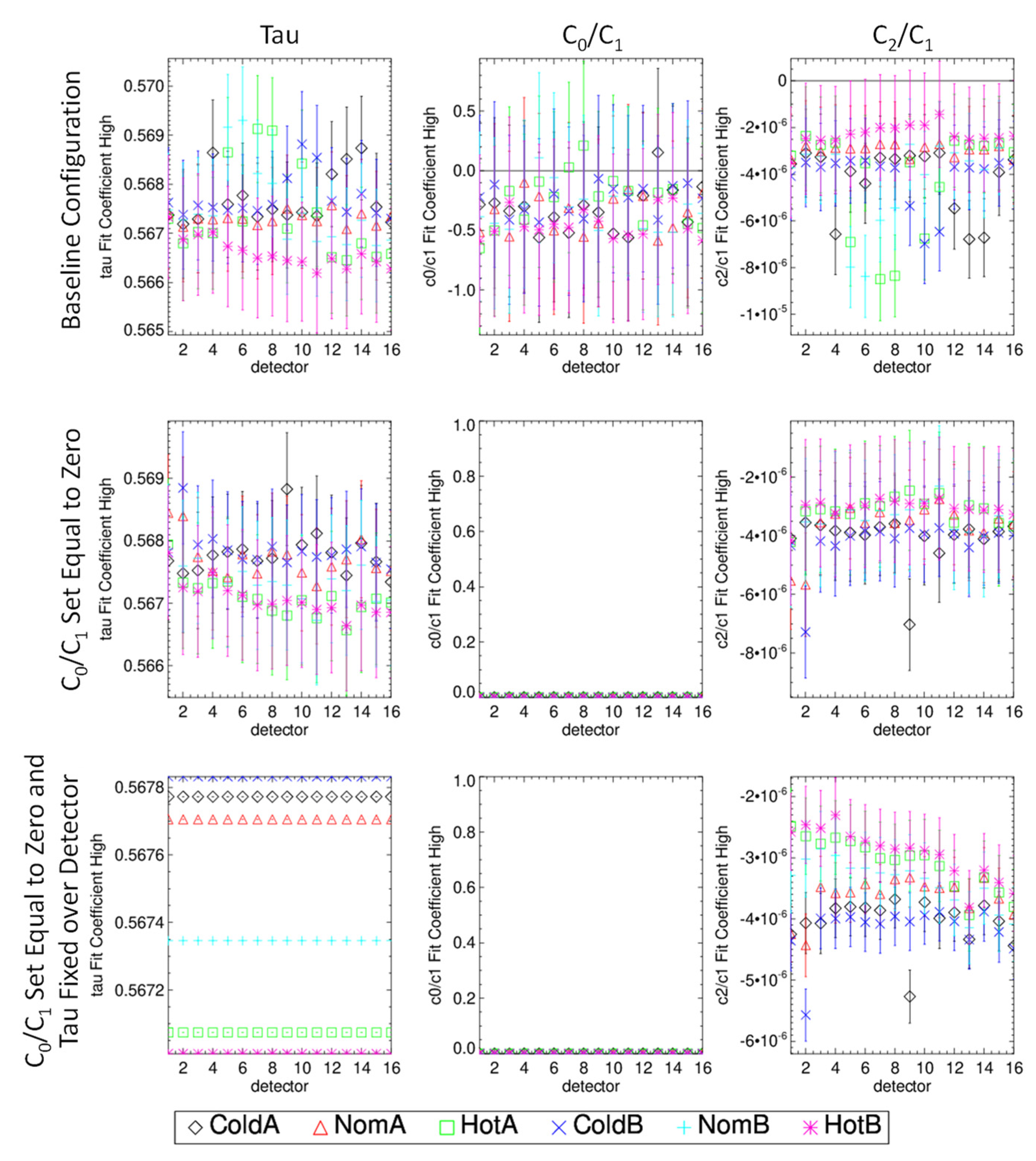
3.4. Detector Response Characterization

The radiometric characterization methodology discussed in Section 2 is used to determine prelaunch calibration coefficients for on-orbit use in the SDR algorithm. Each band, detector, HAM side, and gain have a set of coefficients computed for each TVAC temperature plateau and primary/redundant electronics side. Figure 13 shows an example of the regression coefficients tau, $\frac{c_0}{c_1}$, and $\frac{c_2}{c_1}$ from the SIS100 measurements for band M1 high gain for all TVAC temperature plateaus’ electronic sides. The first column corresponds to the tau coefficients as a function of the detector with the different colors corresponding to the six-temperature plateau and electronic side combinations, the second column $\frac{c_0}{c_1}$, and the third $\frac{c_2}{c_1}$. The rows show the results for the different HAM sides with the first being HAM A and the second HAM B. Whiskers on the points represent the two-sigma uncertainty in the coefficients using the covariance matrix of the least squares regression shown in Equation (6). The assumption is that the tau coefficient should be a constant value across detector and temperature plateau since the physical construction of the LAA should not be angularly dependent or have temperature or electronic sensitivities. These tau variations in Figure 13 are then assumed to be residual uncertainties of the fitting regression being placed in the tau term. An anticorrelated behavior of the $\frac{c_2}{c_1}$ coefficient across the detector and plateau with respect to the tau term indicates that the errors are balanced between these two fitting terms. When the tau for a detector is higher than its counterparts, the $\frac{c_2}{c_1}$ coefficient is below its corresponding detector counterparts. This indicates that some of the detector response in the SIS100 measurements has higher-order nonlinear characteristics than the $\frac{c_2}{c_1}$ coefficient and is being balanced by the tau coefficient. The TMCSIS measurement data show even more of the nonlinear residual fit error in its coefficients, as seen in Figure 14 for band M1 low gain. This could be due to TMCSIS illumination non-uniformity across the track direction; collimated versus diffuse illumination conditions between the TMCSIS and SIS100, respectively; or TMCSIS source instability during LAA in and out collects. The $\frac{c_0}{c_1}$ fit regression term contains information about measurement errors at the low range, where biases, such as nonlinearity, can affect the offset. The model used for characterizing the detector’s response assumes that, at zero radiance, the dns should be zero. Dark noise, nonlinearity, or compensation for higher-order response features can cause the $\frac{c_0}{c_1}$ term to be nonzero. Evaluating the two sigma uncertainties of the $\frac{c_0}{c_1}$ coefficients in comparison with the zero value is used to determine whether the coefficients should be set to zero or left as a calibration coefficient parameter. If the uncertainties bound the zero axis, then the $\frac{c_0}{c_1}$ information is assumed to be dark noise or other minor errors that should not be included in the calibration. Large $\frac{c_0}{c_1}$ values indicate that $\frac{c_0}{c_1}$ is compensating for nonlinearity or other significant response influence and should be included in the calibration coefficients.

An example of fitting coefficients, for the VNIR bands, is shown in Figure 15 for band M1, HAM A in high gain for all temperature and electronic configurations. The first row shows the fit results with no constraints on the coefficients; the second row fixed $\frac{c_0}{c_1}$ to zero; the third fixed tau to the detector, plateau, and electronic side average; and $\frac{c_0}{c_1}$ fixed to zero. The first row shows how error contributors due to higher-order nonlinearity, offset biases, source instabilities, and other contributors cause the tau to be detector and configuration dependent, $\frac{c_0}{c_1}$ to be less than zero, and $\frac{c_2}{c_1}$ to have anticorrelated behavior with the tau term. The second row, where $\frac{c_0}{c_1}$ is fixed to zero, has a minimal effect on the tau and $\frac{c_2}{c_1}$ terms but is impactful on low radiance Earth scenes, where a small $\frac{c_0}{c_1}$ bias can have a significant impact on the estimated top-of-atmosphere SDR radiance. It can even result in nonphysical negative radiance SDR values. The on-orbit calibration coefficients used in the SDR processing set $\frac{c_0}{c_1}$ equal to zero to eliminate this effect. The third row, where the tau is fixed to an average of detector and sensor configuration, has a significant effect on the magnitude and detector-to-detector shape of the $\frac{c_2}{c_1}$ nonlinear term. Fixing the tau causes the $\frac{c_2}{c_1}$ term to be more consistent in both the detector and sensor configurations. Since the tau is expected to be constant across detector and sensor configuration, the $\frac{c_2}{c_1}$ values in row 3 are believed to be more representative of the actual detector’s nonlinear behavior. The last row combines the fixed tau across detectors and $\frac{c_0}{c_1}$ equal to zero and is the configuration of choice for the VNIR calibration coefficient fit regression.

The SWIR band’s response versus SIS100 radiance did not match the VNIR band’s behavior with Figure 16 and Figure 17 comparing the fit residuals of band M7 low gain with band M8 single gain for HAM side A, respectively. The y-axis is the fit residual based on the least squares regression of Equation (6), and the x-axis is the SIS100 radiance. The different color symbols correspond to the different detectors for that band. The band M7 fit residuals, in Figure 16, are on the order of ±0.15%, while the band M8 fit residuals, in Figure 17, are ±0.5% at low radiances. There is also a visible nonlinear residual error at low radiance scenes for the band M8 fit that is not present in the M7 values. An investigation by the vender found that this nonlinearity was a result of an improper voltage bias on the SWIR focal plane. This required the regression fits for the SWIR bands to have a $\frac{c_3}{c_1}$ term to account for higher nonlinear behavior. Equation (10) shows how this additional term is added to Equation (6).

$$d{n}_{in}=\left({\tau }_{LAA}-1\right)\frac{c_0}{c_1}+{\tau }_{LAA}d{n}_{out}+\frac{c_2}{c_1}\left({\tau }_{LAA}d{n}_{out}^2-d{n}_{in}^2\right)+\frac{c_3}{c_1}\left({\tau }_{LAA}d{n}_{out}^3-d{n}_{in}^3\right)$$

(10)

Equation (10) was then used to perform the regression in a similar fashion as the VNIR bands. Figure 18 shows the band M8 fit residuals, like Figure 17, using the third-order polynomial regression fit. The residuals at the lower radiance region and above a radiance of 50 show improvement over the second-order model. A fourth-order polynomial fit (not shown here) improved the performance even more than the third order, but the on-orbit SDR algorithm does not support it. Therefore, a third-order regression model was used to compute the SWIR band calibration coefficients for the on-orbit SDR LUTs. Figure 19 shows an example of band M8, HAM A fit coefficients in a similar style to the band M1 values in Figure 15. The first row is the coefficients with no fixed parameters, the second row $\frac{c_0}{c_1}$ is set to zero, the third row has the tau fixed to the detector, and $\frac{c_0}{c_1}$ fixed to zero. The anticorrelation behavior between the tau and $\frac{c_2}{c_1}$ is consistent with the VNIR bands, but now the $\frac{c_3}{c_1}$ term shows a strong correlation with the tau. Fixing $\frac{c_0}{c_1}$ equal to zero does not greatly influence the tau, $\frac{c_2}{c_1}$, or $\frac{c_3}{c_1}$, but it does improve the low radiance calibration by not including low signal test artifacts. Fixing the tau brings both the $\frac{c_2}{c_1}$ and the $\frac{c_3}{c_1}$ coefficients closer together over sensor configuration and detector but also changes the magnitude of their values. It is also interesting to note that the $\frac{c_2}{c_1}$ and the $\frac{c_3}{c_1}$ coefficients maintain their anticorrelation with respect to one another when the tau is fixed. The last row, where both $\frac{c_0}{c_1}$ and the tau are fixed, is the configuration for fit coefficient used to assess the SWIR radiometric performance. The characterization of band I3 showed that detector 4 was not within the uncertainties of the other 31 bands and is considered a “bad detector” for on-orbit SDR applications. This is consistent with the blinking behavior observed in the SNR measurements.

3.5. Response Sensitivity to Instrument Temperature

The response change versus EM or focal plane temperature is measured during the transitions between TVAC plateaus. The rate of change in the response versus the delta temperature of either the EM or focal plane change is computed and as a correction to the calibration coefficients. With on-orbit calibration measurements only at the South Pole, intraorbital temperature corrections of the calibration coefficients are required. Figure 20 and Figure 21 show an example of the band M1 response change (δL) as a function of temperature change (δT) for the EM and optomechanical module (OMM), respectively, during the transition between cold and nominal plateaus. Each symbol represents a measurement captured during the plateau transition, and each color corresponds to a detector within band M1. The fit lines in the figures are used to model the temperature sensitivities for requirements assessment and on-orbit look-up table (LUT) creation. The focal plane sensitivity for band M1 is on the order of 0.012 W/m²/sr/µm per 1 K change in temperature. The on-orbit variations within one orbit are on the order of 2 K. This indicates that the impact of the response sensitivity to temperature is around 0.024 W/m²/sr/µm or less within an orbit. The band M1 response sensitivity to the EM is around 0.0007 W/m²/sr/µm over a 1 K range. Orbital EM temperature variation within an orbit is ~0.5 K or less, making the temperature sensitivity of the response to the EM temperature almost negligible.

Table 5. VIIRS radiometric sensitivity to temperature change of the instrument. Columns 2 and 3 are for electronics module and optomechanical module temperature sensitivities for the TVAC transition from cold to nominal plateaus and columns 4 and 5 are the corresponding sensitivities for the nominal-to-hot plateau transition.

	Cold-to-Nominal		Nominal-to-Hot
	dL/dT EM	dL/dT OMM	dL/dT EM	dL/dT OMM
I1	0.0161	0.0762	0.0065	0.0291
I2	−0.0014	−0.0207	−0.0057	−0.0531
I3	0.0018	−0.0052	−0.0005	−0.0155
M1	−0.0007	−0.0120	−0.0002	−0.0145
M2	0.0000	−0.0074	0.0010	−0.0111
M3	−0.0006	−0.0114	0.0007	−0.0158
M4	0.0012	−0.0159	−0.0002	−0.0197
M5	−0.0008	−0.0128	−0.0010	−0.0138
M6	0.0006	−0.0041	0.0002	−0.0075
M7	−0.0011	−0.0177	−0.0012	−0.0186
M8	0.0014	−0.0221	0.0002	−0.0263
M9	0.0046	0.0071	−0.0181	0.0031
M10	0.0013	−0.0063	−0.0018	−0.0182
M11	0.0015	0.0010	0.0000	−0.0024

lists the temperature sensitivities for all the bands for both the EM and OMM.

3.6. Uncertainty

The RSB reflectance uncertainty is broken down into six contributors to the total uncertainty. Figure 22 shows the reflectance accuracy error tree contributors that are root sum squared (RSSed) into the top-level accuracy value. Each one of the boxes in Figure 22 has subcategories that are listed in

Table 6. A breakout of the reflective solar band calibration uncertainty tree for each component and a total rollup (highlighted in green for pass and red for fail). Band M11 fails due to high uncertainty in the SD BRF characterization.

Description	Error Type	M1		M2		M3		M4		M5		M6	M7		M8	M9	M10	M11	I1	I2	I3
		Low	High	Low	High	Low	High	Low	High	Low	High		Low	High
Reflectance Accuracy (RSS of Bias & Random Totals)		1.90	1.88	1.78	1.74	1.88	1.68	1.41	1.37	1.38	1.41	1.50	1.43	1.42	1.76	1.48	1.37	2.25	1.36	1.35	1.37
Characterization Uncertainty at Ltyp	Random	0.24	0.05	0.46	0.31	0.85	0.19	0.45	0.31	0.32	0.43	0.67	0.49	0.49	1.14	0.36	0.21	0.59	0.23	0.18	0.13
Response Stability	Random	0.140	0.140	0.120	0.120	0.110	0.110	0.120	0.120	0.130	0.130	0.120	0.120	0.130	0.130	0.220	0.200	0.120	0.130	0.120	0.190
Offset Knowledge & Stability	Random	0.040	0.010	0.040	0.010	0.030	0.012	0.040	0.014	0.040	0.040	0.090	0.040	0.010	0.040	0.030	0.020	0.070	0.070	0.045	0.060
Spec Unc Alloc	Random	0.00	0.00	0.00	0.00	0.00	0.00	0.00		0.00	0.00	0.00	0.00	0.00	0.00	0.00	0.00	0.00	0.00	0.00	0.00
RVS Unc Alloc		0.71	0.71	0.25	0.25	0.06	0.06	0.07	0.07	0.1	0.1	0.06	0.06	0.06	0.13	0.49	0.1	0.09	0.09	0.06	0.08
Pre-Launch Char Uncer	Random	0.10	0.10	0.06	0.06	0.05	0.05	0.06	0.06	0.08	0.08	0.04	0.05	0.05	0.12	0.48	0.07	0.08	0.07	0.05	0.04
Polarization Error	Random	0.00	0.00	0.00	0.00	0.00	0.00	0.00	0.00	0.00	0.00	0.00	0.00	0.00	0.00	0.00	0.00	0.00	0.00	0.00	0.00
RVS Change over Life	Random	0.70	0.70	0.24	0.24	0.04	0.04	0.03	0.03	0.06	0.06	0.04	0.03	0.03	0.06	0.08	0.07	0.04	0.06	0.03	0.07
SD Uncertainty		1.74	1.74	1.69	1.69	1.67	1.66	1.33	1.33	1.33	1.33	1.33	1.33	1.33	1.33	1.33	1.33	2.16	1.33	1.33	1.34
Pre-Launch SD BRDF	Random	0.76	0.76	0.76	0.76	0.76	0.76	0.76	0.76	0.76	0.76	0.76	0.76	0.76	0.76	0.76	0.76	0.76	0.76	0.76	0.76
Straylight	Bias	0.63	0.63	0.63	0.63	0.63	0.63	0.63	0.63	0.63	0.63	0.63	0.63	0.63	0.63	0.63	0.63	0.63	0.63	0.63	0.63
M11 BRDF Extrapolation	Random	0.00	0.00	0.00	0.00	0.00	0.00	0.00	0.00	0.00	0.00	0.00	0.00	0.00	0.00	0.00	0.00	1.70	0.00	0.00	0.00
Other SD		1.43	1.43	1.38	1.37	1.34	1.34	0.89	0.89	0.89	0.89	0.89	0.89	0.89	0.89	0.9	0.89	0.9	0.89	0.89	0.91
SD Degradation over Life	Random	0.12	0.07	0.13	0.07	0.10	0.04	0.10	0.04	0.10	0.04	0.04	0.09	0.03	0.09	0.13	0.09	0.16	0.08	0.10	0.20
SD - Sun Angle Uncertainty	Random	0.33	0.33	0.33	0.33	0.33	0.33	0.33	0.33	0.33	0.33	0.33	0.33	0.33	0.33	0.33	0.33	0.33	0.33	0.33	0.33
Post-Launch BRF Change	Random	0.50	0.50	0.50	0.50	0.50	0.50	0.50	0.50	0.50	0.50	0.50	0.50	0.50	0.50	0.50	0.50	0.50	0.50	0.50	0.50
SAS Error	Random	0.24	0.24	0.24	0.24	0.24	0.24	0.24	0.24	0.24	0.24	0.24	0.24	0.24	0.24	0.24	0.24	0.24	0.24	0.24	0.24
SDSM Error		0.79	0.79	0.68	0.68	0.61	0.61	0.61	0.61	0.61	0.61	0.61	0.61	0.61	0.61	0.61	0.61	0.61	0.61	0.61	0.61
Baseline SDSM Test	Random	0.61	0.61	0.61	0.61	0.61	0.61	0.61	0.61	0.61	0.61	0.61	0.61	0.61	0.61	0.61	0.61	0.61	0.61	0.61	0.61
Spectral OOB	Bias	0.50	0.50	0.30	0.30	0.07	0.07	0.03	0.03	0.00	0.00	0.00	0.00	0.00	0.00	0.00	0.00	0.00	0.00	0.00	0.00
Lunar Cal Error	Random	1.00	1.00	1.00	1.00	1.00	1.00	0.00	0.00	0.00	0.00	0.00	0.00	0.00	0.00	0.00	0.00	0.00	0.00	0.00	0.00

for all the RSBs. The values in Table 6 come from sensor-level testing, subassembly measurements (SD, SDSM), and modeled data (lunar, straylight). The main contributor to the on-orbit reflectance accuracy is the uncertainty in the SD bidirectional reflectance factor (BRF) and the ability of the SDSM to track the change in the BRF. All the bands, excluding band M11, meet the reflectance accuracy uncertainty requirement of 2%. The characterization of the band M11 BRF had higher uncertainty due to limitations of the vendor’s measurement equipment at 2.25 µm. The higher M1 BRF uncertainty is due to the inability of the characterization equipment to directly measure the BRF at that wavelength and, therefore, required extrapolation. More detail on the M11 extrapolation can be found in [18]. The SD BRF characterization is a key component to the instrument’s on-orbit calibration and is performed independently for each instrument build before launch. Differences in the SD BRF characterization methodologies between instruments can cause on-orbit biases in their SDR radiance values. A comparison of the S-NPP and JPSS-1 VIIRS SDR radiances shows a 2–3% difference. An SDR bias study was performed and showed that the S-NPP VIIRS instrument used a different SD BRF prelaunch characterization setup compared with JPSS-1 VIIRS and likely caused the bias between them [19]. The prelaunch characterization of the RVS is very good (less than 0.3%), but the band M1 values in Table 6 include modeled on-orbit degradation that increases the value to 0.71% at the sensor’s end of life. The uncertainty from the calibration coefficients, temperature sensitivity, and response drift between SD calibrations are small contributors to the total uncertainty. This is a testament to the prelaunch calibration test equipment and measurement methodology.

4. Conclusions

The JPSS-1 VIIRS reflective solar band radiometric performance was evaluated before launch during TVAC testing at three different temperature plateaus. The dynamic range, signal-to-noise ratio, dual gain switching, gain temperature sensitivity, and calibration characterization were discussed. Two bands, I3 and M8, failed to meet the dynamic range requirements with bands I3, M6, and M8 having saturation rollover effects that can impact the SDR performance at very bright scenes. The SNRs for all bands met the requirements with band I3 detector 4 being out of family. Meanwhile, band I3 detector 4 still met the SNR requirement, and the calibration uncertainty was large and caused it to be deemed a bad detector. The sensor requirements allowed one detector on a focal plane to be bad, and therefore, there was no requirement failure. The remaining RSBs mt their calibration coefficient uncertainty requirements, as shown in Table 6. Improvements to the calibration coefficient fits was performed for on-orbit applications. This included forcing the offset coefficient to zero and fixing the transmission of the prelaunch attenuator screen across the detector to improve the consistency of the second or fit coefficient over the detector. A third-order polynomial coefficient was added to the SWIR calibration coefficients to better capture the nonlinear response in the low radiance regions. The radiometric uncertainty of the RSBs is within the 2% requirements except for band M11. This is due to how the SD BRF characterization was performed for this band that increased its characterization uncertainty. While not a requirement, the temperature sensitivity of the detector’s response was characterized. The sensitivity was shown to be small with the EM having little effect on response and the OMM temperature being the main driver of temperature-dependent detector response change. These temperature effects are included in the on-orbit SDR calibration coefficient LUTs to reduce calibration uncertainty within an orbit and over different seasons.

References

1. Wolfe, R.E.; Lin, G.; Nishihama, M.; Tewari, K.P.; Tilton, J.C.; Isaacman, A.R. Suomi NPP VIIRS prelaunch and on-orbit geometric calibration and characterization. J. Geophys. Res. Atmos. 2013, 118, 11508–11521. [Google Scholar] [CrossRef] [Green Version]
2. Holben, B.N.; Kaufman, Y.J.; Kendall, J.D. NOAA-11 AVHRR visible and near-IR inflight calibration. Int. J. Remote Sens. 1990, 11, 1511–1519. [Google Scholar] [CrossRef]
3. Salomonson, V.V.; Barnes, W.; Xiong, J.; Kempler, S.; Masuoka, E. An overview of the Earth Observing System MODIS instrument and associated data systems performance. In Proceedings of the IEEE International Symposium on Geoscience and Remote Sensing, Kuala Lumpur, Malaysia, 17–22 July 2022; pp. 1174–1176. [Google Scholar]
4. Kramer, H.J. Observation of the Earth and Its Environment: Survey of Missions and Sensors, 4th ed.; Springer: Berlin, Germany, 2002; ISBN 3540423885. [Google Scholar]
5. Xiong, X.; Aldoretta, E.; Angal, A.; Chang, T.; Geng, X.; Link, D.; Salomonson, V.; Twedt, K.; Wu, A. Terra MODIS: 20 years of on-orbit calibration and performance. J. Appl. Rem. Sens. 2020, 14, 037501. [Google Scholar] [CrossRef]
6. Xiong, X.; Wenny, B.N.; Barnes, W.L. Overview of NASA Earth Observing Systems Terra and Aqua Moderate Resolution Imaging Spectroradiometer Instrument Calibration Algorithms and On-orbit Performance. J. Appl. Remote Sens. 2009, 3, 032501. [Google Scholar]
7. Cao, C.; De Luccia, F.; Xiong, X.; Wolfe, R.; Weng, F. Early On-Orbit Performance of the Visible Infrared Imaging Radiometer Suite Onboard the Suomi National Polar-Orbiting Partnership (S-NPP) Satellite. IEEE Trans. Geosci. Remote Sens. 2013, 52, 1142–1156. [Google Scholar] [CrossRef] [Green Version]
8. Choi, T.; Cao, C.; Blonski, S.; Wang, W.; Uprety, S.; Shao, X. NOAA-20 VIIRS Reflective Solar Band Postlaunch Calibration Updates Two Years In-Orbit. IEEE Trans. Geosci. Remote Sen. 2020, 58, 7633–7642. [Google Scholar] [CrossRef]
9. Murgai, V.; Johnson, L.; Moskun, E. BRDF Characterization of Solar Diffuser for JPSS J1 using PASCAL. In Proceedings of the Earth Observing Systems XIX, San Diego, CA, USA, 18–20 August 2014; SPIE: Bellingham, WA, USA, 2014; Volume 9218, pp. 346–355. [Google Scholar] [CrossRef]
10. Fulbright, J.; Lei, N.; Efremova, B.; Xiong, X. Suomi-NPP VIIRS Solar Diffuser Stability Monitor Performance. IEEE Trans. Geosci. Remote Sens. 2016, 54, 631–639. [Google Scholar] [CrossRef]
11. Lei, N.; Chiang, K.; Xiong, X. Examination of the angular dependence of the SNPP VIIRS solar diffuser BRDF degradation factor. In Proceedings of the Earth Observing Systems XIX, San Diego, CA, USA, 18–20 August 2014; SPIE: Bellingham, WA, USA, 2014; Volume 9218, pp. 550–562. [Google Scholar]
12. Moyer, D.; McIntire, J.; Oudrari, H.; McCarthy, J.; Xiong, X.; De Luccia, F. JPSS-1 VIIRS Pre-Launch Response Versus Scan Angle Testing and Performance. Remote Sens. 2016, 8, 141. [Google Scholar] [CrossRef] [Green Version]
13. Thuillier, G.; Hersé, M.; Foujols, T.; Peetermans, W.; Gillotay, D.; Simon, P.C.; Mandel, H. The Solar Spectral Irradiance from 200 to 2400 nm as Measured by the SOLSPEC Spectrometer from the Atlas and Eureca Missions. Sol. Phys. 2003, 214, 1–22. [Google Scholar] [CrossRef]
14. Cao, C.; Zhang, B.; Shao, X.; Wang, W.; Uprety, S.; Choi, T.; Blonski, S.; Gu, Y.; Bai, Y.; Lin, L.; et al. Mission-Long Recalibrated Science Quality Suomi NPP VIIRS Radiometric Dataset Using Advanced Algorithms for Time Series Studies. Remote Sens. 2021, 13, 1075. [Google Scholar] [CrossRef]
15. Oudrari, H.; McIntire, J.; Xiong, X.; Butler, J.; Lee, S.; Lei, N.; Schwarting, T.; Sun, J. Prelaunch Radiometric Characterization and Calibration of the S-NPP VIIRS Sensor. IEEE Trans. Geosci. Remote Sens. 2015, 53, 2195–2210. [Google Scholar] [CrossRef]
16. Zhang, B.; Cao, C.; Uprety, S.; Shao, X. NOAA-20 VIIRS radiometric band saturation evaluation and comparison with Suomi NPP VIIRS using global probability distribution function method. In Proceedings of the Earth Observing Systems XXIII, San Diego, CA, USA, 19–23 August 2018; SPIE: Bellingham, WA, USA, 2018; Volume 10764, pp. 505–512. [Google Scholar] [CrossRef]
17. Wang, W.; Cao, C.; Blonski, S.; Gu, Y.; Zhang, B.; Uprety, S. An Improved Method for VIIRS Radiance Limit Verification and Saturation Rollover Flagging. IEEE Trans. Geosci. Remote Sens. 2022, 60, 5403011. [Google Scholar] [CrossRef]
18. Murgai, V.; Klein, S. Spectralon Solar Diffuser BRDF extrapolation to 2.25 microns for JPSS J1, J2, and J3. In Proceedings of the Earth Observing Systems XXIV, San Diego, CA, USA, 11–15 August 2019; SPIE: Bellingham, WA, USA, 2019; Volume 11127, pp. 75–85. [Google Scholar] [CrossRef]
19. Moyer, D.; Uprety, S.; Wang, W.; Cao, C.; Guch, I. S-NPP/NOAA-20 VIIRS reflective solar bands on-orbit calibration bias investigation. In Proceedings of the Earth Observing Systems XXVI, Virtual Conference, 3 August 2021; SPIE: Bellingham, WA, USA, 2021; Volume 11829, pp. 319–321. [Google Scholar] [CrossRef]
Figure 1. VIIRS horizontal sampling interval (HSI) for a VIIRS moderate band as a function of scan angle. The light blue and green lines show the unaggregated pixel growth along-scan for the scan and track directions, respectively. The dark blue line shows the pixel growth for the scan direction with the three aggregation zones.
Remotesensing 14 05113 g001
Figure 2. VIIRS scan section diagram illustrating the different collection regions and their angles during a single scan.
Remotesensing 14 05113 g002
Figure 3. Diagram of the VIIRS solar diffuser calibration. This includes the VIIRS scanner that looks at the Earth and solar diffuser (SD) when illuminated by the Sun through an attenuation screen and the solar diffuser stability monitor (SDSM) that views the Sun through a screen and the SD while it is illuminated.
Remotesensing 14 05113 g003
Figure 4. A cartoon of the VIIRS TVAC test chamber setup. The SV, TMCBB, and SIS100 sources are shown with respect to the instrument location within the chamber.
Remotesensing 14 05113 g004
Figure 5. A comparison of the on-orbit solar spectral irradiance profile and the SIS100 radiance profile. The OOB RSR contributions are not weighted the same in on-orbit and prelaunch applications.
Remotesensing 14 05113 g005
Figure 6. Band M4 dynamic range measurements for all detectors, legend in the upper right, for HAM side B. The points to the left of the first vertical line are high gain measurements. The band switches to low gain after a radiance of 40. The first and second vertical red lines are for high and low gain Lmax, respectively. The y-axis is offset subtracted VIIRS response, and the x-axis is the SIS100 radiance during the measurement.
Remotesensing 14 05113 g006
Figure 7. Band M8 dynamic range measurements for all detectors, legend in the upper right, for HAM side A. The y-axis is offset subtracted VIIRS response, and the x-axis is the SIS100 radiance during the measurement. The vertical red line corresponds to Lmax, and the saturation occurs before the line. The rollover in the response is due to saturation of the focal plane electronics. This causes two unique radiance levels to produce the same VIIRS digital number.
Remotesensing 14 05113 g007
Figure 8. Band I3 dynamic range measurements for all detectors, legend on the right, for HAM side B. The y-axis is offset subtracted VIIRS response, and the x-axis is the SIS100 radiance during the measurement. The vertical red line corresponds to Lmax, and the saturation occurs before the line. The rollover in the response is due to saturation of the focal plane electronics. This causes two unique radiance levels to produce the same VIIRS digital number. The blue crosses are from detector 4 that is an out of family with degraded performance that has continued on orbit.
Remotesensing 14 05113 g008
Figure 9. Band M6 dynamic range measurements for all detectors, legend in the upper right, for HAM side B. The y-axis is offset subtracted VIIRS response, and the x-axis is the SIS100 radiance during the measurement. The vertical red line corresponds to Lmax, and the saturation occurs before the line. The rollover in the response is due to saturation of the focal plane electronics. This causes two unique radiance levels to produce the same VIIRS digital number.
Remotesensing 14 05113 g009
Figure 10. Band M7 digital numbers (DNs) as a function of scan during prelaunch testing (upper image). The pattern shows the detector’s response to the SIS100 profile as it scans across it in auto gain mode. The wings on the left and right are high gain DNs (blue line), where the detector is partially viewing the SIS100 aperture. When the DNs reach the gain switch point value, the detector switches to low gain and the DNs drop in the middle of the image (orange line). The M7 radiance is shown in the middle image and is the upper image DNs’ converted radiance using the prelaunch calibration coefficients. The lower image is a zoom-in of the gain transition point to show that it is continuous in radiance.
Remotesensing 14 05113 g010
Figure 11. The signal-to-noise ratio (SNR) of band I3 for all detectors (colored symbols) as a function of SIS100 radiance (W/m2/µm/sr). The three vertical red lines are for Lmin (left), Ltyp (middle), and Lmax (right). The decrease in SNR at the Lmax line is due to partial saturation of the signal. This behavior is used help identify valid response data for characterization purposes.
Remotesensing 14 05113 g011
Figure 12. The signal-to-noise ratio (SNR) of band M10 for all detectors (colored symbols) as a function of SIS100 radiance (W/m2/µm/sr). The three vertical red lines are for Lmin (left), Ltyp (middle), and Lmax (right).
Remotesensing 14 05113 g012
Figure 13. Band M1 high gain fit coefficients for all detectors (x-axis) and TVAC/electronics configurations (colors and symbols). The columns are tau, c 0 c 1 , and c 2 c 1 . The rows are HAM A and B. Cold, nominal, and hot plateaus and electronics sides A and B are shown here.
Remotesensing 14 05113 g013
Figure 14. Band M1 low gain fit coefficients for all detectors (x-axis) and TVAC/electronics configurations (colors and symbols). The columns are tau, c 0 c 1 , and c 2 c 1 . The rows are HAM A and B. Cold, nominal, and hot plateaus and electronics sides A and B are shown here.
Remotesensing 14 05113 g014
Figure 15. Band M1 high gain fit coefficients for all detectors (x-axis) and TVAC/electronics configurations (colors and symbols) for HAM A. The columns are tau, c 0 c 1 , and c 2 c 1 . The rows are not fixed parameters, c 0 c 1 fixed at zero, c 0 c 1 fixed at zero, and the tau set to the detector average of each plateau. Cold, nominal, and hot plateaus and electronics sides A and B are shown here.
Remotesensing 14 05113 g015
Figure 16. Band M7 low gain fit residuals as a function of SIS100 radiance within the Lmin and Lmax regions for all detectors (colors and symbols).
Remotesensing 14 05113 g016
Figure 17. Band M8 fit residuals as a function of SIS100 radiance within the Lmin and Lmax regions for all detectors (colors and symbols) using a second-order polynomial fit.
Remotesensing 14 05113 g017
Figure 18. Band M8 fit residuals as a function of SIS100 radiance within the Lmin and Lmax regions for all detectors (colors and symbols) using a third-order polynomial fit.
Remotesensing 14 05113 g018
Figure 19. Band M8 fit coefficients for all detectors (x-axis) and TVAC/electronics configurations (colors and symbols) for HAM A. The columns are tau, c 0 c 1 , c 2 c 1 , and c 3 c 1 . The rows are not fixed parameters, c 0 c 1 fixed at zero, c 0 c 1 fixed at zero, and the tau set to the detector average of each plateau. Cold, nominal, and hot plateaus and electronics sides A and B are shown here.
Remotesensing 14 05113 g019
Figure 20. Band M1 temperature sensitivity (dL) as a function of electronics module (EM) temperature change between nominal and hot plateau for each detector (colors and symbols).
Remotesensing 14 05113 g020
Figure 21. Band M1 temperature sensitivity (dL) as a function of focal plane assembly (FPA) temperature change between nominal and hot plateau for each detector (colors and symbols).
Remotesensing 14 05113 g021
Figure 22. VIIRS top-level radiometric calibration uncertainty tree.
Remotesensing 14 05113 g022