Abstract
Intermittent records of satellite soil moisture data are major obstacles that constrain their hydrometeorological applications. Based on the European Space Agency Climate Change Initiative (ESA CCI) soil moisture combined product, two machine learning models were employed to reconstruct soil moisture in China during 1979–2019 in both temporal and spatial domains, and latent errors for reconstructed series, as well as their performances for tracing climate extremes, were analyzed. The results showed that with the homogeneity of available data over space, the spatial approach performed well in reproducing the spatial heterogeneity of soil moisture (with medians of the correlation coefficient (CC) above 0.8 and root mean square errors (RMSEs) ranging from 0.02 to 0.03 m3∙m−3). The temporal approach (CC values of 0.7 and RMSEs ranging between 0.02 and 0.03 m3∙m−3) was superior in capturing the seasonality features and the timely and accurate mapping of short-term soil moisture dynamics impacted by rainstorms. However, both approaches failed to identify the location and severity of droughts accurately. The findings highlight the benefits of combining the strengths of both temporal and spatial gap-filling approaches for improving the estimation of missing values and hydrometeorological applications.
1. Introduction
Soil moisture, defined as the water stored within the unsaturated soil zone, is a key variable for understanding the Earth system process [1]. As a major component in the hydrological cycle, soil moisture governs the partition of precipitation into runoff and infiltration, controls the available water in land for evapotranspiration, and also has a notable impact on the climate system through land–atmosphere feedback [2,3]. Given its important role in linking water and energy movements, soil moisture has a wide range of applications, serving as a critical parameter for climate projection, hydrological process simulation, and monitoring hydro-meteorological extreme events (e.g., floods, heatwaves, and droughts) [4,5,6,7]. A long-term series of soil moisture with broad spatial extent and continuous temporal coverage is a prerequisite for the above applications.
Values of soil moisture can be obtained from three major sources, i.e., ground measurements, Earth system model simulations, and satellite observations. With digital/electrical signals collected from ground instruments, probes, or sensors installed, in situ observations inarguably are the ideal options for accurate estimates of soil water content for a target site. The quality of ground observations is largely subject to the operation of sampling devices and measuring methods; meanwhile, sparse observation sites/networks are also an obvious drawback in terms of reflecting the spatial heterogeneity of soil moisture [8]. For large-scale soil moisture monitoring, land surface modeling offers an alternative which simulates the terrestrial exchange process of water and energy fluxes through various physically based numerical models. Uncertainties associated with model structure, parameterization, and meteorological forcings are major issues to be solved to improve the accuracy of soil moisture estimation. With successively launched new satellite missions, remotely sensed soil moisture products have increasingly emerged during the past two decades. The Soil Moisture Active Passive (SMAP) satellite from the National Aeronautics and Space Administration (NASA), the Soil Moisture and Ocean Salinity (SMOS) satellite mission led by the European Space Agency (ESA), and the ESA Climate Change Initiative (CCI) are representative blended products that provide global soil moisture retrievals at fine temporal resolutions [9,10,11,12]. With the abilities of providing soil moisture estimations over a wide spatial extent, these remote-sensing-based products have been widely used for monitoring large-scale soil moisture dynamics. However, some inherent issues such as the low spatial and temporal resolutions, as well as missing values, are major problems often encountered in remotely sensed soil moisture products due to Radio Frequency Interference (RFI) effects, thick cloud coverages, dense vegetation impacts, or satellite sensor errors [13,14].
To ensure the continuity of long-term satellite observations, many efforts have been devoted to filling the gaps in intermittent soil moisture records. These include the merging of multiple datasets (e.g., the integration of various satellite products, as seen in the ESA CCI product), applications of various mathematic algorithms and statistical models for gap-filling or missing value reconstruction, the assimilation of satellite observations into land surface models, along with improvements in such interpolation techniques for advancing data accuracy and their fractional coverages [13,15,16,17,18]. The generation of spatially consistent and temporally continuous soil moisture products therefore becomes a key issue among these progresses given the highly variable nature of soil moisture across temporal and spatial scales [19]. For example, Wang et al. [20] employed a penalized least square method to simultaneously consider information over time and space, but the data accuracy is discounted when large spatial heterogeneity exists. Ford et al. [21] compared six temporal interpolation methods and found the artificial neural network (ANN) method is less impacted by data density and is the most accurate and stable method. Meanwhile, the Daily Average Replacement method could also be an alternative when strong temporal autocorrelation exists. In a different manner, reconstructions in the spatial domain mainly rely on information from other pixels of the same image to infer missing values [22]. Geostatistical methods such as the kriging and inverse distance weighting method are representatives of the spatial gap-filling approaches. In addition, simple and multiple linear regression, as well as machine learning models, have also been applied for the spatial reconstruction of missing values [16]. Although both temporal and spatial approaches are able to reproduce the continuity of a dataset for different purposes of usage, they essentially follow different rules of infilling the missing values in the arithmetic, and their performances depend on the spatial and temporal deficiency of the information and signal characteristics (e.g., seasonality, amplitude, or variance) of the intermittent dataset be complemented.
However, it is rare for studies to have comprehensively compared the performances of the temporal and spatial approaches in filling data gaps [16,21,22,23,24], as well as their strengths and limitations in capturing the dynamics of soil moisture at both short and long time scales. The aim of this study, therefore, is to bridge this research gap. An evaluation of the temporal and spatial gap-filling techniques was performed for the ESA CCI soil moisture product by using two machine learning models, i.e., the ANN and the random forest (RF), given their wide applications for infilling missing values (e.g., Cui et al. [25]; Yuan et al. [26]; Abowarda et al. [27]). The remainder of this study is organized as follows: Section 2 describes the temporal and spatial coverage of the ESA CCI soil moisture product in China and auxiliary data used in this study. At the same time, Section 2 introduces the principle of the two machine learning models and how we reconstructed the soil moisture series in the temporal and spatial domains. Section 3 presents the results obtained by different models in the temporal and spatial domains and their performances in tracing the dynamics of soil moisture during landfall typhoon and drought events. A discussion of the major findings is provided in Section 4. Conclusions from this study are drawn in Section 5.
2. Materials and Methods
2.1. Soil Moisture Products
2.1.1. ESA CCI SM
The European Space Agency’s Soil Moisture Climate Change Initiative (CCI) project provides global satellite-observed soil moisture (SM) datasets by merging soil moisture retrievals from various active-microwave-based and passive-microwave-based sensors. Remote sensing data acquired from satellites are spatially resampled and temporally resampled to generate data products with a spatial resolution of 0.25 degrees and a temporal resolution of one day. After its first release in 2012, this product has experienced qualitative improvements by introducing new satellite-sensor-based datasets and enhanced merging algorithms, and it is updated at regular intervals [12,13]. Three types of daily surface soil moisture products at a spatial resolution of 0.25 degree were provided by the ESA CCI SM, including the ACTIVE product (merging soil moisture retrievals from active-microwave-based sensors), the PASSIVE product (merging soil moisture retrievals from passive-microwave-based sensors), and the COMBINED product (merging soil moisture retrievals from both active-microwave-based and passive-microwave-based sensors). In this study, the COMBINED product of ESA CCI SM in version v04.4 (https://www.esa-soilmoisture-cci.org/, accessed on 4 November 2021) generated by an improved uncertainty characterization approach for better parameterizing the triple collocation merging scheme was employed [28,29]. The soil moisture data are provided in volumetric units (m3∙m−3). Figure 1 shows the spatiotemporal coverage of available ESA CCI SM data in China from 1979 to 2019. It is evident that the spatial coverage of SM data increases over time, especially for the period after 2006, with more sensors and instruments incorporated (e.g., AMSR-E and ASCAT) to construct the ESA CCI SM; the mean percentage of available data in China reached 50% during 2007−2019 (Figure 1a). The significant spatial heterogeneity of data coverage is seen for the study area, where pixels in western Xizang and eastern the Xinjiang are the ones with the lowest percentage of data, and the northern China has highest coverage of available data, ranging between 60 and 70% (Figure 1b). For the temporal distribution, the data coverage is generally high (ranges between 50% and 60%) in growing seasons (namely the Days of Year (DOY) 120−300), while large gaps (with coverage below 20%) are observed in winter (Figure 1a). On the basis of coverage inspection, the soil moisture data (version 04.4) from 1979 to 2019 during the growing season (April−October) were chosen for analysis.
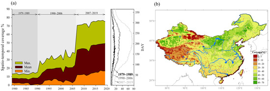
Figure 1.
(a) Maximum, mean, and minimum coverage of available ESA CCI SM data in China and the distribution (i.e., the Days of Year (DOYs)) of data coverage over multiple years. (b) Fractional coverage of available data for each grid in China during 1979−2019.
2.1.2. ERA-Interim Reanalysis
The ERA-Interim reanalysis (Nanjing, China, Dee et al. [30]; https://apps.ecmwf.int/, accessed on 6 November 2021) is a global atmospheric product produced by the European Centre for Medium-Range Weather Forecasts (ECMWF) based on a sequential data assimilation scheme. This dataset provides daily soil moisture data of four depths (0−7 cm, 7−28 cm, 28−100 cm, and 100−289 cm), with a spatial resolution of 0.75 degrees. Meanwhile, ECMWF also provides other optional interpolated data with different spatial resolutions. For temporal coverage, the dataset covers the period from 1979 until the present. In this study, records of the topsoil layer (0−7 cm) at a 0.25° (25 kilometers) spatial resolution during 1979−2019 were employed for intercomparison.
2.1.3. In Situ Soil Moisture Measurements
Given the dense distribution of agrometeorological stations over China (a total of 778 stations) and their relatively complete and long data records, the in situ soil moisture observations of the China agrometeorological stations were employed for validation. The dataset of these stations contains information regarding crop growth and soil moisture content for farmland and can be downloaded from the China Meteorological Data Sharing Service System (Nanjing, China, http://data.cma.cn/, accessed on 8 November 2021). The in situ soil moisture was measured based on the principle of Frequency Domain Reflectometry (FDR) in which the dielectric constant of a certain volume element around the sensor can be obtained by measuring the operating frequency of an oscillating circuit. The capacitance probes were installed at a vertical angle (90°) for the depths of 10, 20, 50, 70, and 100 cm, respectively. The probes contained a waterproof enclosure, sensing head, and a cable. With a temporal resolution of ten days, the data were provided in units of saturation degree (%), and was available from January 1992 to December 2013. After quality checkup, 298 out of 778 sites (generally evenly distributed in the mainland of China, as shown in Figure 2) with relatively complete records of the first soil layer (0−10 cm) were selected. These included 36 sites in arid zones, 143 sites in semi-arid zones, 105 sites in semi-humid zones, and 14 sites in humid zones. Since the unit of the in situ soil moisture data is different from that of ESA CCI SM, the degree of saturation (%) was converted to volumetric soil moisture content (m3∙m−3) using the following equation:
where θv represents the volumetric soil moisture content (m3∙m−3), s represents the degree of saturation (%), and f is a map of the porosity [31], which was estimated based on the Harmonized World Soil Database (HWSD).
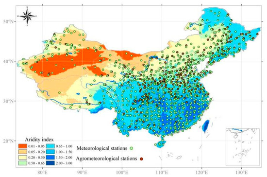
Figure 2.
Spatial distribution of the national meteorological stations and Chinese agrometeorological stations and climate zones.
2.2. Ancillary Data
The daily ground-based meteorological observations, including precipitation and air temperature from the 756 national meteorological stations (Figure 2), were collected from the China Meteorological Administration (CMA, Nanjing, China; http://data.cma.cn/, accessed on 8 November 2021). Based on the inverse distance weighting interpolation method, these daily point-scale precipitation and air temperature observations during 1979 to 2019 were processed into gridded data at a spatial resolution of 0.25° (25 kilometers).
The third-generation NDVI (NDVI3g) dataset released by Global Inventory Modeling and Mapping Studies (GIMMS) was collected from the NASA Ames ecological forecasting lab (Nanjing, China, http://ecocast.arc.nasa.gov/da-ta/pub/gimms/3g.v1/, accessed on 10 November 2021). It is currently the latest version of the GIMMS NDVI product with the longest time series of data available and also presents higher quality in mid-high latitudes than other versions [32]. The spatial resolution of this dataset was 0.083° (10 kilometers), and the data were resampled into 0.25° × 0.25° (25 kilometers × 25 kilometers) to match the resolution of gridded meteorological forcings and soil moisture data. The NDVI3g was available semimonthly through 1982−2015, and they were generated into daily time series (e.g., days for the first half of the month share the same NDVI3g value and were estimated to be another value for the second half of the month) to meet the time step requirements of machine learning.
The global land surface satellite leaf area index (GLASS LAI) product released by the Center for Global Change Data Processing and Analysis of Beijing Normal University (Nanjing, China, http://www.bnu-datacenter.com/, accessed on 11 November 2021) was employed as the input of the machine learning model. Compared to other existing LAI products, the GLASS LAI provides global data with improved temporal smoothness and better agreement with ground measurements [33]. The GLASS LAI product has a temporal resolution of eight days and spans from 1981 to 2017. During 1981−1999, the LAI product was generated from AVHRR reflectance data at a spatial resolution of 0.05° (5.5 kilometers), while for the period of 2000−2019, the LAI product was derived from Moderate Resolution Imaging Spectroradiometer (MODIS) surface-reflectance data at a spatial resolution of 1 km. In this study, the GLASS LAI data during 1981−2017 was employed, and the original series with a temporal resolution of eight days were processed into daily series, as were the daily NDVI3g. For spatial preprocessing, the product was resampled to a 0.25° (25 kilometers) spatial resolution using the nearest-neighbor resampling method.
The soil texture parameter was estimated based on the Harmonized World Soil Database (HWSD), which was developed by the Food and Agriculture Organization (FAO) and the International Institute for Applied Systems Analysis (IIASA) [34]. Version 1.1 of the HWSD contains four source databases, including the European Soil Database (ESDB), various regional SOTER databases, the Soil Map of the World, and the recent 1:1,000,000 scale soil map of China provided by the Institute of Soil Science, Chinese Academy of Sciences [35]. This database provides soil properties for the topsoil (0–30 cm) and subsoil (30–100 cm) separately. For soil texture, it is divided into 13 classes (e.g., sand, clay, and loam) according to a particular range of separate soil (i.e., clay, silt, and sand) fractions. The spatial resolution of the HWSD is 30 arc-second. In this study, the soil texture pixels in China were extracted and resampled into a 0.25° (25 kilometers) spatial resolution with the nearest-neighbor resampling method.
In addition, five geographic and topographic properties, including the geographical coordinates (denoted by the latitude and longitude), altitude, slope, and aspect for each pixel were also extracted for analysis. The elevation information was obtained from the shutter radar topography mission digital elevation model (SRTM, Nanjing, China, http://srtm.csi.cgiar.org/, accessed on 12 November 2021), and its spatial resolution was 0.08333° (10 kilometers). The slope and aspect for each grid cell were derived from elevation on the geospatial information system platform. All these data were resampled into a spatial resolution of 0.25° (25 kilometers) by using the nearest-neighbor resampling method.
2.3. Machine Learning
2.3.1. Random Forest
Random forests (RF), developed by Breiman [36] and Cutler et al. [37], is a nonparametric and ensemble machine learning technique, being the worldwide preference for classification or regression purposes. Compared to other existing machine learning methods, RF exhibits high efficiency and fast processing speed for handling high-dimensional datasets, and it is apt at modeling the complex and nonlinear relationships between predicators and responsible variables [38].
Specifically, the algorithm combines the bagging idea (or the bootstrapping technique) and the random selection of features to construct a multitude of decision trees with controlled variance at the training phase. Each decision tree is independently built from a random subset of the same training samples, and the final predicted values are produced by the aggregation of the results of all the individual decision trees that make up the forest. Obviously, the samples to be learned are separated into two parts, in which two thirds of the samples (also referred to as in-bag samples) are used for model construction, and the remaining one third (also referred to as out-of-the bag (OOB) samples) are employed to estimate the error of the resulting RF model (which is known as the OOB error) based on the mean squared error (MSE). Before fitting the RF model, two tuning parameters need to be specified, i.e., the number of decision trees (or tree size) to be generated, and the number of features to be selected and tested when growing the trees [38]. Several previous studies highlighted that the classification accuracy is insensitive to the tree size, and a number of 500 decision trees were mostly used by the majority of relevant studies [39,40]. According to the performance of the OOB error, in this study, the tree size and the number of features were set to 1000 and three, respectively.
2.3.2. Artificial Neural Network
ANNs, also simply referred to as neural networks (NNs), are a machine learning technique inspired by the biological neural networks that constitute brains. The training of NNs follows a supervised learning algorithm which involves successive adjustments until the processed output of the network (often a prediction value) infinitely approaches to a target output. To deal with various tasks, a multitude of different NN frameworks have been developed. Among these, the back propagation neural network (BPNN) is one typical form of the learning algorithms which trains feedforward neural networks and has been widely applied to solve nonlinear issues [16,41].
A BPNN is constituted by a multilayer architecture in which at least one hidden layer is configured to connect the input and output layers. Each layer may include several nodes or neurons, and two nodes in each adjacent layer are directly connected, represented by a weighted value to show their relational degree. With the aim of finding a suit of weights to ensure the output vector produced by the network sufficiently close to the desired output vector, the BPNN uses the steepest gradient descent method to train the multilayer networks through both forward and backward propagations. In the forward process, neurons in the input layer pass through each hidden layer with a result derived in the output layer. If the generated values do not close to the expected results, then the backward pass would start by iteratively updating weights and thresholds of neurons in each hidden layer until a minimum sum of squared errors is achieved [26,42].
In this study, a three-layer (i.e., one input, hidden, and output layer, respectively) BPNN was employed to simulate the relationship between the explanatory variables and soil moisture. The architecture was equipped with ten neurons in the input layer, thirteen neurons in the hidden layer, and one neuron in the output layer. Specifically, ten neurons in the input layer were the possible factors that might explain the variability in soil moisture, including geographic and topographic features (i.e., central latitude, central longitude, DEM, slope, and aspect), meteorological forcings (i.e., precipitation and temperature), vegetation conditions (i.e., NDVI and LAI), and soil texture. The number of neurons in the hidden layer was an empirical value, and the gradient descent of the momentum method was adopted to train the network. Based on previous research [43,44] and numerical simulation experiments, the learning rate, maximum interaction, and target error were set to 0.01, 1000, and 0.001, respectively. These parameters could ensure the robust behavior of the model with optimal simulation results, and they were also less time consuming. The neurons of the output layer were the soil moisture series.
2.4. Reconstruction of Soil Moisture in the Temporal and Spatial Domains
Machine learning has been increasingly used for gap-filling or the reconstruction of intermittent soil moisture series. For a certain region, the variation in soil moisture essentially is a three-dimensional issue that has features both in time and space (Figure 3). According to the way that the patterns are discovered from the data deluge, the target dataset can be reconstructed in the temporal and spatial domains, respectively. The red grid cell (30.68 °N, 106.1 °E) in the data cube in Figure 3 represents an example of the ESA CCI soil moisture product with data gaps during 1979−2019. To obtain serially complete soil moisture records, reconstruction in the temporal domain mainly relies on the gap-free explanatory variables (e.g., meteorological variables and vegetation conditions that may provide useful information on the temporal dynamics of soil moisture) for the target grid cell and the temporal structure explored by the machine learning models. With the constructed relationship, missing values of pixels could be predicted and filled up by mapping temporally varying features into target variables. As for the spatial domain, the objective was to complete each daily map of the CCI SM series. As shown in Figure 3, the missing value on 13 August, 2000 could be filled up with information extracted from the data deluge which consists of gap-free ancillary data and spatially discontinuous soil moisture data on the specific day. It is worth mentioning that although the auxiliary data from grid cells in the research domain all participate as model inputs, their roles in the prediction of the missing values would be different, and higher weights would be allocated to the neighboring grid cells. In this study, the ANN and RF models were employed to reconstruct the ESA CCI SM series in the temporal and spatial domains, with four seamless soil moisture series derived, denoted as ANNt, ANNs, RFt, and RFs. To evaluate the performances of different methods as well as different models, the soil moisture values were randomly separated into the training and the test subsets (80% and 20% of the existing values, respectively). Two evaluation coefficients were employed for the validation assessment with the test set, i.e., the Pearson correlation coefficient (CC) and the root mean square error (RMSE), and higher values of CC and smaller absolute values of RMSE suggest good performances.
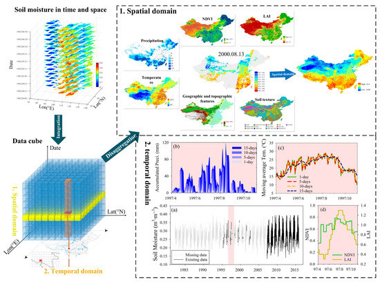
Figure 3.
A sketch map of reconstructing soil moisture in the temporal and spatial domains. (a) Soil moisture in the temporal domain. (b) Accumulated precipitation in the temporal domain. (c) Moving average temperature in the temporal domain. (d) NDVI and LAI in the temporal domain.
3. Results
3.1. Performances Evaluation of the Machine Learning Approaches
Figure 4 compares the reconstructed soil moisture series under 12 scenarios against original ESA CCI SM series. These included the ANN and RF simulated soil moisture series by using the training subset, the test subset, and the entire dataset in the temporal (denoted as ANNt_cal, ANNt_ver, ANNt_all, RFt_cal, RFt_ver, and RFt_all) and spatial (denoted as ANNs_cal, ANNs_ver, ANNs_all, RFs_cal, RFs_ver, and RFs_all) domains, respectively. It can be seen that the medians of CC obtained in the spatial domain were all above 0.8, and the medians of RMSE ranged from 0.02 to 0.03 m3∙m−3. The accuracies for the temporal domain were slightly lower, where the medians of CC generally reduced by 0.1 to 0.2 compared to those in the spatial domain. In terms of RMSE values, very tiny differences were found between the temporal and spatial context. As for the performances of the two machine learning models, the RF outperformed the ANN given high CC values and low RMSE values both in the spatial and temporal domains. The performances of the ANN presented considerable deviations under different scenarios, particularly for the spatial domain, and significant differences were observed among ANNs_cal, ANNs_ver, and ANNs_all. It can be seen that the results of ANNs_cal derived from 80% of existing data for model training were very close to ANNs_all, while large deviations (the CC values varied between 0.4 and 0.95) were obtained for ANNs_ver. In contrast, the CC and RMSE values of six RF reconstructed soil moisture series were generally comparable, and RF was therefore more robust than the ANN.
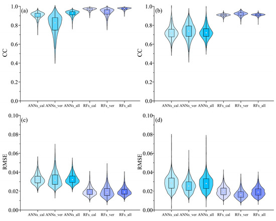
Figure 4.
Comparison of reconstructed soil moisture series in different scenarios against original ESA CCI SM series. (a,b) are the CC values for the spatial and temporal domains, respectively, and (c,d) are corresponding RMSE values.
Table 1 further compares the statistics of the ANN and RF reconstructed soil moisture series in the temporal and spatial domains (the entire data were employed for training, and are denoted as ANNt, ANNs, RFt, and RFs, respectively) against the in situ soil moisture observations of the China agrometeorological stations and ERA data in four climate zones. Observations of the in situ soil moisture sites located in the same grid cell were aggregated into average values for comparison. In terms of mean values, the ERA presented overestimations in semi-humid areas with a bias of 0.06 m3∙m−3. In contrast, the mean values of the original ESA CCI series and the four machine-learning-based series were generally close to those of in situ observations. Exceptions were found in humid areas, where soil moisture was conformably underestimated by the original ESA CCI series and the four machine-learning-based series, with the bias being no more than 0.04 m3∙m−3. As for the extremum (i.e., the maximum and minimum values), the ANN and RF presented good results in arid and semi-humid areas with relatively low bias obtained compared to the in situ observations. Especially for RFt and RFs, the biases of maximum and minimum values were no more than 0.04 m3∙m−3 in absolute values. In semi-arid areas, the biases for all six grid-based soil moisture series (including ERA and five ESA CCI related series) were slightly higher compared to the extremum of in situ observations. One possible reason lies in the fact that the semi-arid zone includes the most in situ sites in China, which may increase the sample errors; meanwhile, geographically, this climate zone spans across approximately 40 longitudes, and the intrinsic defects of a remotely sensed SM product associated with image/stripes fusion may be largely exposed given the wide spatial coverage in longitudes [14]. In humid areas, the systematic negative bias of the ESA CCI SM series was further amplified for the minimum values, and such underestimation was not improved by the two machine models, either. The humid areas in China are mostly covered with dense vegetation, which affects the remotely sensed SM quality [12,45]. In addition, the unsatisfactory performances of the ANN and RF suggest the present input variables (e.g., NDVI and LAI) are insufficient to reflect the complicated variation in soil moisture, and the incorporation of other information, such as the soil moisture condition on the previous/following day in the temporal domain [21] or the combination of multiple data sources to overcome the inherent bias from the original ESA CCI product, may possibly improve the simulation accuracies.

Table 1.
Comparison of reconstructed soil moisture series against in situ soil moisture observations of the China agrometeorological stations and ERA data.
3.2. Comparison of Spatial and Temporal Reconstructed Series
Figure 5 compares the average values of reconstructed soil moisture series obtained in the spatial and temporal domains by using the ANN and RF models over China and in four climate zones. It can be seen that for both models, the soil moisture series derived in the spatial domain presented larger variabilities than those in the temporal domain, and this difference was particularly significant in humid areas. As shown in Figure 5m,n, the values of temporally reconstructed soil moisture series in humid zones mainly varied between 0.3 and 0.34 m3∙m−3, while the cases in the spatial context exhibited large fluctuations, with soil moisture values ranging between 0.34 and 0.2 m3∙m−3. It is worth mentioning that the ESA CCI soil moisture product had rather low data coverage in southern China before the 1990s (Figure 1). Such an irregular distribution of available data may influence the filled results and even produce some outliers when using the spatial gap-filling approach. A detailed analysis of the effects of sample size is presented in the discussion section. In contrast, small differences were found in the arid zone given the small variation ranges in soil moisture (0.12~0.22 m3∙m−3) in this region (Figure 5d,e). In addition, the two machine learning models also performed differently in the spatial and temporal domains. Compared to the ANN, there was generally a good agreement between temporally and spatially reconstructed series with RF. As for the ANN, the spatially simulated values on the whole were lower than those obtained in the temporal domain (with scatters mostly distributed below the 1:1 line), particularly in arid and humid zones (Figure 5f,o).
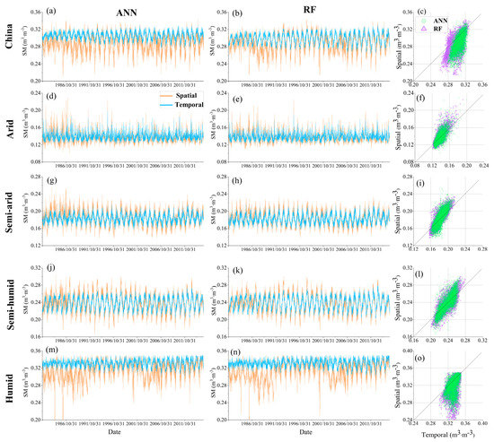
Figure 5.
Comparison of reconstructed soil moisture series in the spatial and temporal domains by using the ANN and RF models over China and in four climate zones. (a,d,g,j,m) The comparison of average values of reconstructed soil moisture series obtained in the spatial and temporal domains by using the ANN model. (b,e,h,k,n) The comparison of average values of reconstructed soil moisture series obtained in the spatial and temporal domains by using the RF model. (c,f,i,l,o) Scatter plot of all spatial values and temporal values in the area.
The ability to capture the seasonal soil moisture dynamics is also an important metric for evaluating the accuracy of obtained results. Figure 6 presents the intra-annual distribution of reconstructed daily soil moisture series in the temporal and spatial domains with the ANN (upper four panels) and RF (bottom four panels) models in four climate zones. Similar patterns were observed for the two machine learning models, where except for the semi-humid region, substantial differences were found between the patterns derived from the temporal and spatial domains. In the arid zone (Figure 6a,e), the temporally reconstructed series suggested soil moisture values were generally high in spring and autumn and low in summer, which was in accordance with the patterns of in situ observations [46]. The series derived from the spatial domain, however, presented an opposite pattern with peak values in summer. Likewise, the temporal reconstruction approach accurately captured the intra-annual dynamics of soil moisture in the semi-arid zone compared with in situ observations [47], while the spatial approach failed to capture the slightly decreasing pattern of soil moisture from the Days of Year (DOYs) 1−130, but generally presented satisfactory performances in the growing seasons. In humid areas, the temporally reconstructed series presented a unimodal pattern with peak values in summer, which was in good agreement with patterns of precipitation. The spatial approach missed this interannual pattern again but presented tiny fluctuations around 0.31 m3∙m−3. The abovementioned results suggest that the temporal approach is superior to the spatial approach in depicting the interannual variation in soil moisture.
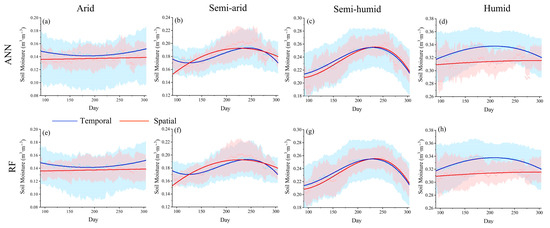
Figure 6.
Distribution of reconstructed daily soil moisture in the temporal and spatial domains with the ANN (a–d) and RF (e–h) models in four climate zones during 1979−2019. The blue and red solid lines are the mean values in each day. The blue and red shades represent the 5% and 95% percentiles of soil moisture in each climate zone.
3.3. Performances for Tracing Typhoon Rainstorm and Drought Extreme Events
Soil moisture is an important variable linking the water cycle in the atmosphere–land interface. Extreme climatic conditions such as typhoon rainstorms or prolonged atmospheric water deficits may lead to varying responses in soil moisture over time and space. In this section, the abilities of the reconstructed soil moisture series for tracing extreme weather–climate events at different time scales were assessed.
3.3.1. Performances for Tracing Typhoon Rainstorm Events
Figure 7 shows the affected areas and migration routes of major typhoons in China during the summer of 2006. Five landfall typhoons successively hit the coastal and inland provinces from 27 June to 10 August, and such a high frequency (equivalent to one landfall typhoon per nine days on average) of landfall typhoons induced heavy casualties and huge economic losses to society. Strong winds and heavy precipitation are two major features during typhoon-affected days, which may lead to large increments in soil moisture through infiltration in a very short period of time. Taking the case of typhoon Bilis as an example, it landed in Taiwan on 13 July; then, the tropical cyclone moved northwestwards, accompanied with rainfall in Fujian and the neighboring provinces within the next five days. This spatiotemporal migration pattern was accurately captured by the temporally reconstructed soil moisture series (Figure 8). It can be seen that both SM_ANNt and SM_RFt presented rapid increments in soil moisture (positive anomalies above 2) in the coastal areas of Fujian province on 14 July; then, the impacted areas expanded gradually and the correlation with rainfall was clear. The variations in SM_ANNs and SM_RFs anomalies, however, presented poor performances and failed to track the landfall location and time of typhoon. The cases for the fifth typhoon Kaemi (from 25 July to 28 July) and sixth typhoon Prapiroon (from 2 August to 6 August) revealed a similar phenomenon, as shown in Figure 8, where the temporally reconstructed soil moisture series allowed the timely and accurate mapping of the areas most affected by typhoons and rainstorms and were superior to the spatially reconstructed soil moisture series in capturing the variation in soil moisture in short time scales (Figure 9).
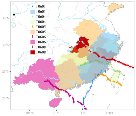
Figure 7.
Affected areas and migration routes of the five major typhoons in 2006.
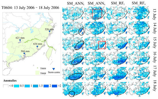
Figure 8.
Spatial variations in anomalies of reconstructed soil moisture series in the temporal and spatial domains with the ANN and RF models (denoted as SM_ANNt, SM_ANNs, SM_RFt, and SM_RFs, respectively) during the fourth typhoon Bilis (from 13 July 2006 to 18 July 2006). The black solid circles show the regions where SM_ANNt accurately capture the increments in soil moisture, and the red solid rectangles show the poor performances of SM_ANNs.
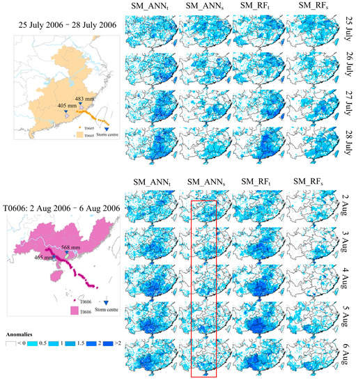
Figure 9.
This is the same as Figure 8, but the fifth typhoon Kaemi (from 25 July to 28 July) and sixth typhoon Prapiroon (from 2 August 2006 to 6 August 2006) are displayed. The red solid rectangle shows the poor performances of SM_ANNs.
3.3.2. Performances for Tracing Drought Events
Unlike typhoons, the formation of droughts usually takes a longer time, but the impacts can be devastating due to their long persistence and wide spatial extents. According to the Bulletin of flood and drought disasters (Nanjing, China, http://www.mwr.gov.cn/, accessed on 20 November 2021) released by the Ministry of Water Resources of the People’s Republic of China (hereafter referred to as the recorded drought information), approximately 17,966,000 hectares on average suffered droughts during 2000−2019 (Figure 10a), and we selected three recent large-scale droughts to investigate the performance of reconstructed series in monitoring the dynamics of soil moisture at long time scales. As shown in Figure 10b, the recorded drought information showed the 2007 drought mainly hit northern China (i.e., Inner Mongolia and Heilongjiang province, with the affected area exceeding 10%), followed by the central and southern regions (the affected area ranged between 1% and 5%). In contrast, the drought condition in western and eastern China was mild, with the affected area being no more than 1%. With respect to the performance of reconstructed soil moisture series, the two spatially derived series generally effectively captured such a spatial pattern of drought. Overestimation was found for the two temporally derived series in southeastern China, especially for the SM_RFt (Figure 11). Again, SM_RFt overestimated the drought condition in eastern China during 2009. For the 2011 drought, underestimation occurred for SM_ANNs and SM_RFs when monitoring the drought condition in southeastern China. SM_ANNt, by contrast, provided more accurate mapping of the affected area and outperformed other derived soil moisture series in the 2011 drought.
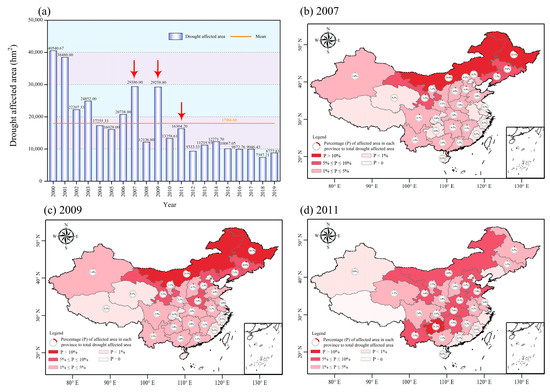
Figure 10.
(a) Annual drought area in China during 2000–2019. (b–d) The percentage of affected area in each province to total drought affected area in China in 2007, 2009, and 2011, respectively. The data were collected from the Bulletin of flood and drought disasters released by the Ministry of Water Resources of the People’s Republic of China. Drought affected areas for each province were not available before 2006 and are marked in light-colored shades in Figure 10a.
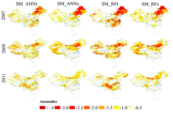
Figure 11.
Spatial distribution of average anomalies of reconstructed soil moisture in the temporal and domains with the ANN and RF models (denoted as SM_ANNt, SM_ANNs, SM_RFt, and SM_RFs) in 2007, 2009, and 2011, respectively.
Obviously, all four reconstructed series presented better performances for monitoring drought conditions in northern, arid regions than in southern, humid regions. Although the temporally based series could accurately capture the drought condition in southern China, the overestimation of droughts was apparent in the southeastern regions. In contrast to the overwhelming advantages in tracing typhoon-induced variation in soil moisture, the temporal approach failed to reproduce its advantage of reflecting soil moisture dynamics at long time scales. One reason may lie in that the input data for model training were mostly variables that reflected the moisture status at momentary or short time scales. Droughts in nature, however, are moisture deficits accumulated at long time scales (e.g., 1 month or longer). In this sense, the ten variables employed for training the model may be insufficient to illustrate the variation in soil moisture at long time scales. The incorporation of more information responsible for the dynamics of soil moisture may possibly improve the accuracy of drought application. For example, the incorporation of large-scale circulation factors, such as the sea temperature and 500 hPa geopotential height, may improve the abilities reflect the variation in prolonged moisture status [48].
4. Discussion
Previous studies mostly focused on the applications and improvements in either temporal or spatial gap-filling techniques to obtain spatially complete and temporally continuous soil moisture series [49,50,51]. However, their differences, as well as the influencing factors for the derived results, have been rarely addressed. Throughout the process of gap-filling, the differentiated performance between the spatial and temporal approaches can be attributed into two aspects. One is from the database, including the gaps in original series, ancillary variables incorporated, and the data cube architecture (arrangement of data information). The other refers to the effectiveness of data-driven models employed for extracting information features from the data cube.
It is well acknowledged that data gaps over time and space influence the interpolation results, while their specific impacts on the temporal and spatial gap-filling approaches have rarely been compared. To address this issue, a sensitivity analysis with a varied sample size was implemented for the RF model given its relatively robust behaviors in estimating missing values (Figure 4 and Figure 5). For the temporal domain, the sub-datasets for model training were generated by an equal-step method (5% increments of data coverage for each step) from 1982 to 2019. Such inverse-order sampling generally follows the way that the missing values were temporally infilled, since more data gaps were concentrated before the 1990s (Figure 1a) due to immature satellite remote sensing technology. Figure 12 shows the CC and RMSE values for the temporally reconstructed series against original series under different percentages of data inputs over China. It can be seen that the accuracy of the reconstructed series increased with the enlarged sample size, and robust estimation results were obtained when 50~60% of available ESA CCI soil moisture data were incorporated for model training. This finding is consistent with previous studies [23,51].
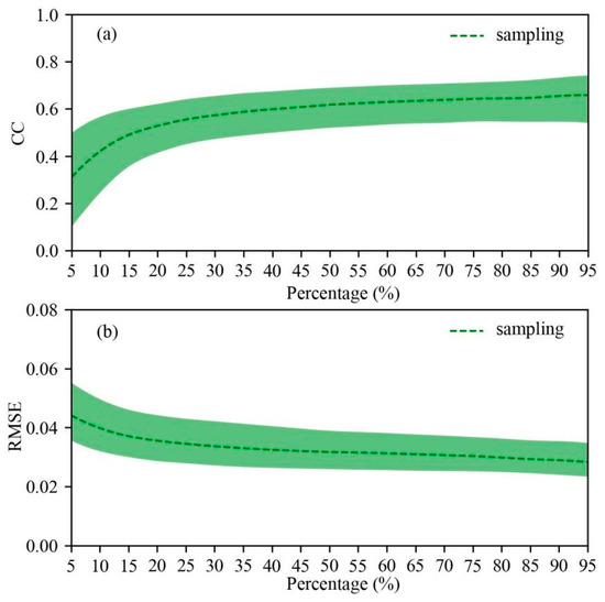
Figure 12.
(a) The correlation coefficients and (b) root mean square errors for the RF gap-filling procedure in the temporal domain under different percentages of data coverage for model training. The dashed lines represent the average results of all grids over China.
The case for the spatial domain is more complicated. Three different spatial sampling methods (including one for the uniform sampling and two for non-uniform sampling) accompanied with varied data lengths were examined. The spatially uniform sampling was realized by an equal space distance searching algorithm (i.e., one sample is taken from every n neighboring point) so that grid cells with disparate properties across the research domain would be selected during the sampling process. Regarding non-uniform sampling, samples were randomly selected from a certain region, meaning that data information in other districts may be lost. As shown in Figure 13, the uniform sampling was less impacted by the sample size and maintained a stable performance (CC and RMSE values varied around 0.8 and 0.05 m3∙m−3, respectively) under varied percentages of data inputs. In contrast, the two cases of non-uniform sampling presented large fluctuations, and the accuracy even decreased with an enlarged sample size. This suggests the spatial uniformity of data selection is more important than gap lengths for the spatial domain. According to Figure 1, the available ESA CCI soil moisture data were unevenly distributed before the 1990s with rather low data coverage in southern China, and such non-uniform information over space may be responsible for the outliers in humid regions (Figure 5m,n). It is worth mentioning that swaths are commonly encountered for remote sensing soil moisture products due to the ascending or descending satellite sensors [12], and the performance of the spatial gap-filling approach could be compromised for areas with large missing values.
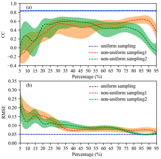
Figure 13.
(a) The correlation coefficients and (b) root mean square errors for the RF gap-filling procedure in the spatial domain under different percentages of data coverage by uniform and non-uniform sampling schemes for model training over China.
The temporal and spatial approaches also behave differently in excavating valid information from the data cube. For temporal gap-filling, procedures were implemented for each grid cell so that ancillary variables providing the daily variabilities were valuable for missing value estimation. In other words, geographic features (i.e., central latitude, central longitude, DEM, slope, and aspect) and soil texture have not been well considered in the temporal domain. A lack of such spatial information may transfer to the estimation results. As shown in Figure 5, the variance in temporally reconstructed series was smaller to that in spatially derived ones. This may lead to the underestimation of the available water capacity (AWC, reflecting the maximum water storage in the root zone that can be used for evapotranspiration) for the soil profile [52]. Apart from variables incorporated, the arrangement of data information also influences estimation accuracy. For example, features extracted from chronological precipitation series can be significantly different from those of spatial images. As with the water source of infiltration in the soil profile, the seasonality and effects of the antecedent moisture condition can be exploited from the time series of precipitation, and this is particularly important for a remote sensing product that provides surface soil moisture values. However, such temporal features can hardly be captured by spatial images. This could be one reason for the relatively poor performance of spatial approaches in tracing extreme flood and drought events (Figure 9 and Figure 11).
Therefore, strategies that benefit from the combination of temporal and spatial gap-filling approaches are promising directions for improving estimation precision. Zhang et al. [51] constructed a three-dimensional database by incorporating spatial images in adjacent eight days and proposed a deep partial reconstruction model to take both spatial and temporal information into consideration. While the attempt was proved to be effective, its ability to monitor soil moisture dynamics at long time scales (e.g., droughts, with an optimum monitoring scale of one month or longer) is debatable given the rather limited temporal patterns involved in the database. In addition, the data-driven models also perform differently when infilling data gaps. In this study, we found RF was superior to the ANN given its robust behaviors both in the temporal and spatial domains. Nonetheless, the intrinsic errors from the original ESA CCI product were not substantially improved through the machine learning model (Table 1), and even may transmit to extended applications such as extreme events monitoring (Figure 11). Such genetic behaviors of estimation errors were also found for other interpolation models [51] and should be addressed in future research.
5. Conclusions
Missing values have always been a problem encountered in remote sensing soil moisture products which comprises their continuity for climate- and hydrology-related applications. The temporal and spatial gap-filling techniques, respectively, can remedy this deficiency, but their differences in terms of missing value estimation, as well as their abilities to trace the dynamics of soil moisture at short (e.g., instantaneous variation in typhoon days) and long time scales (e.g., annual variation in drought years), have been seldom compared and evaluated. In this study, a comprehensive comparison between the temporal and spatial gap-filling techniques was performed for the ESA CCI soil moisture combined product in China during 1979–2019. This was implemented by using two machine learning models, i.e., the ANN and RF, to infill the missing values of the ESA CCI soil moisture product in the temporal and spatial domains, respectively, with four reconstructed series derived (i.e., ANNt, ANNs, RFt, and RFs). The results show that the temporal and spatial approaches behaved differently in reproducing the continuity of the long-term soil moisture series.
The temporally based approach had the advantage of precisely capturing the seasonality of soil moisture in different climate zones but was insufficient to fully exhibit the spatial heterogeneity with small variation ranges in soil moisture. For extreme hydro-meteorological monitoring, the temporally based series (i.e., ANNt and RFt) enabled the provision of the timely and accurate mapping of the areas most impacted by typhoons and rainstorms. However, to trace the dynamics of soil moisture at long time scales (i.e., drought events), their superiority was discounted, with better performances in northern arid regions than in southeastern regions. The sensitivity test on varied data gaps suggested the accuracy of estimation increased with a gradually reduced gap length for model training, and robust estimation results can be achieved when 50%–60% of existing ESA CCI soil moisture data were incorporated.
Except for the semi-humid areas, the spatial gap-filling approach did not perform well in capturing the seasonality of soil moisture. Particularly in arid and humid zones, the spatially reconstructed series (i.e., ANNs and RFs) virtually presented no seasonality with tiny fluctuations for the intra-annual distribution. In semi-arid areas, they missed the slightly decreasing pattern of soil moisture in winter (from DOY 1 to 130) but performed pretty well in growing seasons. With higher variance for the reconstructed series, the spatial approach outperformed the temporal approach in reflecting the spatial heterogeneity of soil moisture. At the same time, however, some outliers were generated in the spatially reconstructed series due to the spatially irregular distribution of available ESA CCI data before the 1990s. In terms of hydro-meteorological extremes monitoring, the spatially based approach hardly exhibited any strengths either for typhoon-induced rainstorm or drought events. Different from the temporal approach, the spatial gap-filling technique was less impacted by the length of data gaps; rather, the homogeneity of available data in space was more important for the high accuracy of soil moisture estimation.
The different performances between the temporal and spatial gap-filling approaches largely rely on the information and data features extracted from the data cube in the temporal and spatial domains, respectively, while the machine learning models act as a tool for extracting such information, and their influences on missing values estimation are generally minor. Nonetheless, the RF model is more recommended for use given its robustness than ANN. The intra-seasonal variability in soil moisture is an important signal for interpreting the evolution process of the Earth system, and from the perspective of practical applications such as tracing hydro-meteorological extremes, the temporal gap-filling technique in conjunction with robust machine learning models (such as RF) are more competent for providing timely and accurate mapping of soil moisture dynamics, which is essential for disaster strategies’ implementation and emergency management. Meanwhile, the strength of the spatial approach in representing the spatial heterogeneity of soil moisture at large scales compensates for the temporal approach, and a deep combination of the temporal and spatial gap-filling approaches might be addressed in future research.
Author Contributions
Writing—original draft, Y.L.; methodology and writing—original draft, R.C. and S.Y.; project administration, L.R.; writing—review and editing, X.Z.; supervision, C.L.; visualization, software, and data, Q.M. All authors have read and agreed to the published version of the manuscript.
Funding
This study was supported by the National Key Research and Development Program approved by the Ministry of Science and Technology, the People’s Republic of China, under Grant No. 2019YFC1510600; the National Natural Science Foundation of China under Grant No. (42171021, U2243203, 41901037); the Fundamental Research Funds for the Central Universities under Grant No. 2019B05214; the Central Guidance for Local Science and Technology Development fund projects (grant no. 2021ZY0027); Hunan Provincial Water Conservancy Science and Technology Project (XSKJ2019081-17); and Guangxi province Key R&D projects (2019AB20003).
Data Availability Statement
ERA CCI SM data used in this study are available (https://www.esa-soilmoisture-cci.org/, Nanjing, China, 4 November 2021). ERA-Interim data used in this study are available through European Centre for Medium-Range Weather Forecasts (https://apps.ecmwf.int/, Nanjing, China, 6 November 2021). Meteorological data are available at China Meteorological Data Service Center (http://data.cma.cn/, Nanjing, China, 8 November 2021). NDVI dataset can be download from Global Inventory Modeling and Mapping Studies (http://ecocast.arc.nasa.gov/da-ta/pub/gimms/3g.v1/, Nanjing, China, 10 November 2021). GLASS LAI can be download from the Center for Global Change Data Processing and Analysis of Beijing Normal University (http://www.bnu-datacenter.com/, Nanjing, China, 11 November 2021). Digital elevation data are available at the website (http://srtm.csi.cgiar.org/, Nanjing, China, 12 November 2021). China’s disaster information can be obtained from the Bulletin of flood and drought disasters released by the Ministry of Water Resources of the People’s Republic of China (http://www.mwr.gov.cn/, Nanjing, China, 20 November 2021). The software is Matlab (version 2019a), and the function packages, including random forest and the artificial neural network, can be downloaded from the website (https://www.mathworks.com, Nanjing, China, 2 July 2021).
Conflicts of Interest
The authors declare that they have no known competing financial interests or personal relationships that could have appeared to influence the work reported in this paper.
References
- Peng, J.; Albergel, C.; Balenzano, A.; Brocca, L.; Cartus, O.; Cosh, M.H.; Crow, W.T.; Dabrowska-Zielinska, K.; Dadson, S.; Davidson, M.W.; et al. A roadmap for high-resolution satellite soil moisture applications–confronting product characteristics with user requirements. Remote Sens. Environ. 2021, 252, 112162. [Google Scholar] [CrossRef]
- Greve, P.; Orlowsky, B.; Mueller, B.; Sheffield, J.; Reichstein, M.; Seneviratne, S. Global assessment of trends in wetting and drying over land. Nat. Geosci. 2014, 7, 716–721. [Google Scholar] [CrossRef]
- Martin, H.; Mueller, B.; Dorigo, W.; Seneviratne, S.I. Using remotely sensed soil moisture for land–atmosphere coupling diagnostics: The role of surface vs. root-zone soil moisture variability. Remote Sens. Environ. 2014, 154, 246–252. [Google Scholar]
- Brocca, L.; Ciabatta, L.; Massari, C.; Moramarco, T.; Hahn, S.; Hasenauer, S.; Kidd, R.; Dorigo, W.; Wagner, W.; Levizzani, V. Soil as a natural rain gauge: Estimating global rainfall from satellite soil moisture data. J. Geophys. Res. Atmos. 2014, 119, 5128–5141. [Google Scholar] [CrossRef]
- Miralles, G.D.; Gentine, P.; Seneviratne, S.I.; Teuling, A.J. Land–atmospheric feedbacks during droughts and heatwaves: State of the science and current challenges. Ann. N. Y. Acad. Sci. 2019, 1436, 19–35. [Google Scholar] [CrossRef]
- Liu, Y.; Zhu, Y.; Ren, L.; Otkin, J.; Hunt, E.D.; Yang, X.; Yuan, F.; Jiang, S. Two Different Methods for Flash Drought Identification: Comparison of Their Strengths and Limitations. J. Hydrometeorol. 2020, 21, 691–704. [Google Scholar] [CrossRef]
- Zhu, Y.; Liu, Y.; Wang, W.; Singh, V.P.; Ren, L. A global perspective on the probability of propagation of drought: From meteorological to soil moisture. J. Hydrol. 2021, 603, 126907. [Google Scholar] [CrossRef]
- Peng, J.; Loew, A.; Merlin, O.; Verhoest, N.E.C. A review of spatial downscaling of satellite remotely sensed soil moisture. Rev. Geophys. 2017, 55, 341–366. [Google Scholar] [CrossRef]
- Entekhabi, D.; Njoku, E.G.; O’Neill, P.E.; Kellogg, K.H.; Crow, W.T.; Edelstein, W.N.; Entin, J.K.; Goodman, S.D.; Jackson, T.J.; Johnson, J.; et al. The Soil Moisture Active Passive (SMAP) Mission. Proc. IEEE 2010, 98, 704–716. [Google Scholar] [CrossRef]
- Liu, Y.Y.; Dorigo, W.A.; Parinussa, R.M.; de Jeu, R.A.M.; Wagner, W.; McCabe, M.F.; Evans, J.P.; van Dijk, A.I.J.M. Trend-preserving blending of passive and active microwave soil moisture retrievals. Remote. Sens. Environ. 2012, 123, 280–297. [Google Scholar] [CrossRef]
- Kerr, Y.; Al-Yaari, A.; Rodriguez-Fernandez, N.; Parrens, M.; Molero, B.; Leroux, D.; Bircher, S.; Mahmoodi, A.; Mialon, A.; Richaume, P.; et al. Overview of SMOS performance in terms of global soil moisture monitoring after six years in operation. Remote Sens. Environ. 2016, 180, 40–63. [Google Scholar] [CrossRef]
- Al-Yaari, A.; Wigneron, J.-P.; Dorigo, W.; Colliander, A.; Pellarin, T.; Hahn, S.; Mialon, A.; Richaume, P.; Fernandez-Moran, R.; Fan, L.; et al. Assessment and inter-comparison of recently developed/reprocessed microwave satellite soil moisture products using ISMN ground-based measurements. Remote Sens. Environ. 2019, 224, 289–303. [Google Scholar] [CrossRef]
- Dorigo, W.; Wagner, W.; Albergel, C.; Albrecht, F.; Balsamo, G.; Brocca, L.; Chung, D.; Ertl, M.; Forkel, M.; Gruber, A.; et al. ESA CCI Soil Moisture for improved Earth system understanding: State-of-the art and future directions. Remote Sens. Environ. 2017, 203, 185–215. [Google Scholar] [CrossRef]
- Gruber, A.; De Lannoy, G.; Albergel, C.; Al-Yaari, A.; Brocca, L.; Calvet, J.-C.; Colliander, A.; Cosh, M.; Crow, W.; Dorigo, W.; et al. Validation practices for satellite soil moisture retrievals: What are (the) errors? Remote Sens. Environ. 2020, 244, 111806. [Google Scholar] [CrossRef]
- Liu, Y.; Yang, Y.; Jing, W. Potential Applicability of SMAP in ECV Soil Moisture Gap-Filling: A Case Study in Europe. IEEE Access 2020, 8, 133114–133127. [Google Scholar] [CrossRef]
- Zhang, L.; Liu, Y.; Ren, L.; Teuling, A.J.; Zhang, X.; Jiang, S.; Yang, X.; Wei, L.; Zhong, F.; Zheng, L. Reconstruction of ESA CCI satellite-derived soil moisture using an artificial neural network technology. Sci. Total Environ. 2021, 782, 146602. [Google Scholar] [CrossRef]
- Crow, W.T.; Wood, E.F. The assimilation of remotely sensed soil brightness temperature imagery into a land surface model using Ensemble Kalman filtering: A case study based on ESTAR measurements during SGP97. Adv. Water Resour. 2003, 26, 137–149. [Google Scholar] [CrossRef]
- Hain, C.R.; Crow, W.T.; Mecikalski, J.R.; Anderson, M.C. An ensemble Kalman filter dual assimilation of thermal infrared and microwave satellite observations of soil moisture into the Noah land surface model. Water Resour. Res. 2012, 48, 11. [Google Scholar] [CrossRef]
- Long, D.; Bai, L.; Yan, L.; Zhang, C.; Yang, W.; Lei, H.; Quan, J.; Meng, X.; Shi, C. Generation of spatially complete and daily continuous surface soil moisture of high spatial resolution. Remote Sens. Environ. 2019, 233, 111364. [Google Scholar] [CrossRef]
- Wang, G.; Garcia, D.; Liu, Y.; de Jeu, R.; Dolman, A.J. A three-dimensional gap filling method for large geophysical datasets: Application to global satellite soil moisture observations. Environ. Model. Softw. 2012, 30, 139–142. [Google Scholar] [CrossRef]
- Ford, T.W.; Quiring, S.M. Comparison and application of multiple methods for temporal interpolation of daily soil moisture. Int. J. Clim. 2014, 34, 2604–2621. [Google Scholar] [CrossRef]
- Siabi, N.; Sanaeinejad, S.H.; Ghahraman, B. Comprehensive evaluation of a spatio-temporal gap filling algorithm: Using remotely sensed precipitation, LST and ET data. J. Environ. Manag. 2020, 261, 110228. [Google Scholar] [CrossRef] [PubMed]
- Liu, Y.; Yao, L.; Jing, W.; Di, L.; Yang, J.; Li, Y. Comparison of two satellite-based soil moisture reconstruction algorithms: A case study in the state of Oklahoma, USA. J. Hydrol. 2020, 590, 125406. [Google Scholar] [CrossRef]
- Jing, W.; Zhang, P.; Zhao, X. Reconstructing Monthly ECV Global Soil Moisture with an Improved Spatial Resolution. Water Resour. Manag. 2018, 32, 2523–2537. [Google Scholar] [CrossRef]
- Cui, Y.; Zeng, C.; Zhou, J.; Xie, H.; Wan, W.; Hu, L.; Xiong, W.; Chen, X.; Fan, W.; Hong, Y. A spatio-temporal continuous soil moisture dataset over the Tibet Plateau from 2002 to 2015. Sci. Data 2019, 6, 247. [Google Scholar] [CrossRef]
- Yuan, Q.; Shen, H.; Li, T.; Li, Z.; Li, S.; Jiang, Y.; Xu, H.; Tan, W.; Yang, Q.; Wang, J.; et al. Deep learning in environmental remote sensing: Achievements and challenges. Remote Sens. Environ. 2020, 241, 111716. [Google Scholar] [CrossRef]
- Abowarda, A.S.; Bai, L.; Zhang, C.; Long, D.; Li, X.; Huang, Q.; Sun, Z. Generating surface soil moisture at 30 m spatial resolution using both data fusion and machine learning toward better water resources management at the field scale. Remote Sens. Environ. 2021, 255, 112301. [Google Scholar] [CrossRef]
- Dorigo, W.; Wagner, W.; Gruber, A.; Scanlon, T.; Hahn, S.; Kidd, R.; Paulik, C.; Reimer, C.; van der Schalie, R.; de Jeu, R. ESA Soil Moisture Climate Change Initiative (Soil_Moisture_cci): Version 03.2 Data Collection; Centre for Environmental Data Analysis: Chilton, UK, 2018. [Google Scholar]
- Gruber, A.; Scanlon, T.; van der Schalie, R.; Wagner, W.; Dorigo, W. Evolution of the ESA CCI Soil Moisture climate data records and their underlying merging methodology. Earth Syst. Sci. Data 2019, 11, 717–739. [Google Scholar] [CrossRef]
- Dee, D.P.; Uppala, S.M.; Simmons, A.J.; Berrisford, P.; Poli, P.; Kobayashi, S.; Andrae, U.; Balmaseda, M.A.; Balsamo, G.; Bauer, P.; et al. The ERA-Interim reanalysis: Configuration and performance of the data assimilation system. Q. J. R. Meteorol. Soc. 2011, 137, 553–597. [Google Scholar] [CrossRef]
- Daniel, H. Introduction to Soil Physics; Academic Press: Cambridge, MA, USA, 2013. [Google Scholar]
- Zhu, Z.; Bi, J.; Pan, Y.; Ganguly, S.; Anav, A.; Xu, L.; Samanta, A.; Piao, S.; Nemani, R.R.; Myneni, R.B. Global Data Sets of Vegetation Leaf Area Index (LAI)3g and Fraction of Photosynthetically Active Radiation (FPAR)3g Derived from Global Inventory Modeling and Mapping Studies (GIMMS) Normalized Difference Vegetation Index (NDVI3g) for the Period 1981 to 2011. Remote Sens. 2013, 5, 927–948. [Google Scholar]
- Xiao, Z.; Liang, S.; Wang, J.; Xiang, Y.; Zhao, X.; Song, J. Long-Time-Series Global Land Surface Satellite Leaf Area Index Product Derived from MODIS and AVHRR Surface Reflectance. IEEE Trans. Geosci. Remote Sens. 2016, 54, 5301–5318. [Google Scholar] [CrossRef]
- Nachtergaele, F.; van Velthuizen, H.; Verelst, L.; Batjes, N.; Dijkshoorn, K.; van Engelen, V.; Fischer, G.; Jones, A.; Montanarella, L.; Petri, M.; et al. Harmonized World Soil Database (Version 1.1); FAO: Rome, Italy; IIASA: Laxenburg, Austria, 2009. [Google Scholar]
- Shi, X.Z.; Yu, D.S.; Warner, E.D.; Pan, X.Z.; Petersen, G.W.; Gong, Z.G.; Weindorf, D.C. Soil Database of 1:1,000,000 Digital Soil Survey and Reference System of the Chinese Genetic Soil Classification System. Soil Horiz. 2004, 45, 129–136. [Google Scholar] [CrossRef]
- Leo, B. Random forests. Mach. Learn. 2001, 45, 5–32. [Google Scholar]
- Adele, C.; Cutler, D.R.; Stevens, J.R. Random forests. In Ensemble Machine Learning; Springer: Boston, MA, USA, 2012; pp. 157–175. [Google Scholar]
- Belgiu, M.; Drăguţ, L. Random forest in remote sensing: A review of applications and future directions. ISPRS J. Photogramm. Remote Sens. 2016, 114, 24–31. [Google Scholar] [CrossRef]
- Guan, H.; Li, J.; Chapman, M.; Deng, F.; Ji, Z.; Yang, X. Integration of orthoimagery and lidar data for object-based urban thematic mapping using random forests. Int. J. Remote Sens. 2013, 34, 5166–5186. [Google Scholar] [CrossRef]
- Du, P.; Samat, A.; Waske, B.; Liu, S.; Li, Z. Random Forest and Rotation Forest for fully polarized SAR image classification using polarimetric and spatial features. ISPRS J. Photogramm. Remote Sens. 2015, 105, 38–53. [Google Scholar] [CrossRef]
- Rumelhart, D.E.; Hinton, G.E.; Williams, R.J. Learning representations by back-propagating errors. Nature 1986, 323, 533–536. [Google Scholar] [CrossRef]
- Zhang, Y.; Wu, L. Stock market prediction of S&P 500 via combination of improved BCO approach and BP neural network. Expert Syst. Appl. 2009, 36, 8849–8854. [Google Scholar]
- Bengio, Y. Practical Recommendations for Gradient-Based Training of Deep Architectures. In Neural Networks: Tricks of the Trade; Springer: Berlin/Heidelberg, Germany, 2012; pp. 437–478. [Google Scholar]
- Shi, Y.; Ren, C.; Yan, Z.; Lai, J. High Spatial-Temporal Resolution Estimation of Ground-Based Global Navigation Satellite System Interferometric Reflectometry (GNSS-IR) Soil Moisture Using the Genetic Algorithm Back Propagation (GA-BP) Neural Network. ISPRS Int. J. Geo-Information 2021, 10, 623. [Google Scholar] [CrossRef]
- Kim, H.; Wigneron, J.-P.; Kumar, S.; Dong, J.; Wagner, W.; Cosh, M.H.; Bosch, D.D.; Collins, C.H.; Starks, P.J.; Seyfried, M.; et al. Global scale error assessments of soil moisture estimates from microwave-based active and passive satellites and land surface models over forest and mixed irrigated/dryland agriculture regions. Remote Sens. Environ. 2020, 251, 112052. [Google Scholar] [CrossRef]
- Lu, G.H.; Kuang, Y.H.; Wu, Z.Y.; He, H. Spatial and temporal characteristic of soil moisture in different climatic regions of China. China Rural. Water Hydropower 2013, 5, 15–19. [Google Scholar]
- Buda, S.; Wang, A.; Wang, G.; Wang, Y.; Jiang, T. Spatiotemporal variations of soil moisture in the Tarim River basin, China. Int. J. Appl. Earth Obs. Geoinf. 2016, 48, 122–130. [Google Scholar]
- Ford, T.W.; Labosier, C.F. Meteorological conditions associated with the onset of flash drought in the Eastern United States. Agric. For. Meteorol. 2017, 247, 414–423. [Google Scholar] [CrossRef]
- Yuan, S.; Quiring, S.M. Comparison of three methods of interpolating soil moisture in Oklahoma. Int. J. Clim. 2017, 37, 987–997. [Google Scholar] [CrossRef]
- Almendra-Martín, L.; Martínez-Fernández, J.; Piles, M.; González-Zamora, Á. Comparison of gap-filling techniques applied to the CCI soil moisture database in Southern Europe. Remote Sens. Environ. 2021, 258, 112377. [Google Scholar] [CrossRef]
- Zhang, Q.; Yuan, Q.; Li, J.; Wang, Y.; Sun, F.; Zhang, L. Generating seamless global daily AMSR2 soil moisture (SGD-SM) long-term products for the years 2013–2019. Earth Syst. Sci. Data 2021, 13, 1385–1401. [Google Scholar] [CrossRef]
- Liu, M.; Zhang, B.; He, X. Climate Rather Than Vegetation Changes Dominate Changes in Effective Vegetation Available Water Capacity. Water Resour. Res. 2022, 58, e2021WR030319. [Google Scholar] [CrossRef]
Publisher’s Note: MDPI stays neutral with regard to jurisdictional claims in published maps and institutional affiliations. |
© 2022 by the authors. Licensee MDPI, Basel, Switzerland. This article is an open access article distributed under the terms and conditions of the Creative Commons Attribution (CC BY) license (https://creativecommons.org/licenses/by/4.0/).