Abstract
Korea has been recognized as an earthquake-safe zone, but over recent decades, several earthquakes, at a medium scale or higher, have occurred in succession in and around the major fault zones, hence there is a need for studying active faults to mitigate earthquake risks. In Korea, research on active faults has been challenging owing to urbanization, high precipitation, and erosion rates, and relatively low earthquake activity compared to the countries on plate boundaries. To overcome these difficulties, the use of aerial light detection and ranging (LiDAR) techniques providing high-resolution images and digital elevation models (DEM) that filter vegetation cover has been introduced. Multiple active fault outcrops have been reported along the Yangsan Fault, which is in the southeastern area of the Korean Peninsula. This study aimed to detect active faults by performing a detailed topographic analysis of aerial LiDAR images in the central segment of the Yangsan Fault. The aerial LiDAR image covered an area of 4.5 km by 15 km and had an average ground point density of 3.5 points per m2, which produced high-resolution images and DEMs at greater than 20 cm. Using LiDAR images and DEMs, we identified a 2–4 m high fault scarp and 50–150 m deflected streams with dextral offset. Based on the image analysis, we further conducted a trench field investigation and successfully located the active fault that cut the Quaternary deposits. The N–S to NNE-striking fault surfaces cut unconsolidated deposits comprising nine units, and the observed slickenlines indicated dextral reverse strike-slip. The optically stimulated luminescence (OSL) age dating results of the unconsolidated deposits indicate that the last earthquake occurred 3200 years ago, which is one of the most recent along the Yangsan Fault.
1. Introduction
Earthquakes prove that the Earth is dynamic and fragile due to their unpredictable nature and the ensuing natural disasters are unavoidable. As humans advanced, earthquakes have caused an increasing amount of damage to civilization, owing to high infrastructure and population densities associated with highly developed and populated cities [1,2,3]. To mitigate earthquake damage, it is necessary to apply civil engineering and architectural building design technologies, such as vibration isolation, vibration control, and anti-vibration measures, and to initiate disaster prevention plans such as evacuation scenarios and post-earthquake recovery plans [1,2]. The seismic hazard assessment (SHA) and earthquake risk map, which can predict earthquake hazards, form the basis for establishing practical policies [1,2,4,5]. The evaluation methods for SHA are probabilistic and deterministic, and paleoseismic data are commonly required for both methods; therefore, a concrete SHA begins with the acquisition of reliable paleoseismic data [4,5,6]. Since the inception of the field of paleoseismology, scientists have performed numerous case studies and investigated various research methods to obtain reliable geological data [7,8,9]. In particular, various scientific techniques have been applied to efficiently search for active faults [10,11]. Active fault detection methodology consists of three major components: remote sensing, geophysical techniques, and field surveys (Figure 1). When remote sensing first emerged, aerial photography was primarily used, and as technology advanced, more efficient techniques covering larger areas became possible using satellite images and digital elevation models (DEMs) [12,13,14,15]. Interferometry from synthetic-aperture radar (InSAR) [16,17,18,19,20,21,22] and light detection and ranging (LiDAR) [23,24,25,26,27,28,29,30,31] can be used to precisely search for active faults by providing higher resolution data than older technologies can. Geophysical techniques are non-destructive methods that provide subsurface information without excavation. An infield survey comprising a 3D trench and large-scale mega trenches is also conducted to extract reliable paleoseismic data that reflect the real geometry and kinematics of active faults [7,32,33,34,35].
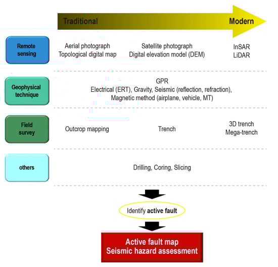
Figure 1.
General methods used in terrestrial paleoseismic investigations. Technological innovations have led to the development of advanced survey techniques, which give the option to select various survey techniques depending on the site-specific condition. Nevertheless, traditional techniques are still needed and used now and can be complemented by modern techniques.
2. Geological Settings
The Korean Peninsula was previously seen as an earthquake-free zone; however, due to the two recent occurrences of medium-scale earthquakes, the Gyeongju earthquake: 09.12.2016, MW 5.5 [36] and Pohang earthquake: 11.15.2017, MW 5.4 [37], there is a need for Korea to prepare for earthquake events. However, limited and low reliability of paleoseismic data, which are essential elements for SHA, exists as a challenge. In the Korean Peninsula, it is difficult to find an active fault due to high humidity, high erosion rate, urbanization, and agriculture [38]. The low reliability of paleoseismic data, due to natural and cultural conditions, is the main limitation to research continuity, which is evidenced by the social evaluation of its effectiveness. Therefore, new techniques and applications that can overcome these local limitations are needed by both policymakers and geologists.
The study of active faults in Korea began with Lee and Na (1983) [39], and a full-scale study was conducted by Okada et al. (1994) [40] in a joint research effort with Japan. Most of the previous studies primarily focused on geological surveys, which form the basis for geotechnical information used to inform the construction of major national infrastructure facilities such as nuclear power plants [41,42]. Since these studies are conducted only when major facilities are built, the connectivity and continuity of the research are poor. The largest challenge is that a comprehensive interpretation of all active faults is limited because faults demonstrating evidence of surface rupture cannot be traced as continuous lines on the map. Previous studies were limited to single-point data such as trenches and outcrops, as such, it was not possible to trace faults in a scientifically evidenced continuous line [43,44,45,46,47,48,49]. The fundamental scientific basis for the search and tracing of active faults is topographic analysis through remote sensing [10]. Practically, remote sensing is a necessary, cost-effective, and efficient research method because it is not possible to physically excavate the full extent of a fault [7,10]. Among the various remote sensing approaches, topographic analysis using LiDAR data makes it possible to precisely trace faults [23,24,25,26,27,28,29,30,31]. In this study, we introduce a topographic analysis using LiDAR in Korea and demonstrate that it is effective and essential when searching for an active fault.
The Korean Peninsula is situated inside the Eurasian Plate, also known as the Amurian Plate [50,51,52,53,54]. Earthquakes do not occur frequently in this area, unlike in Japan, China, Taiwan, and the Philippines, which are neighboring countries located on the plate boundary [55]. Following the scientific observation and instrument measurement of earthquakes, several medium-scale earthquakes have been recorded, and historic paleoseismological and seismic studies suggest the possibility of large-scale earthquakes having occurred in the past [37,56,57,58,59,60,61]. In the current Korean Peninsula stress field, the maximum horizontal principal stress in the E–W and ENE–WSW direction is a result of the far-field stress caused by the collision between the Indian and Eurasian Plates and the subduction angle of the Pacific Plate [62,63]. The overall uplift rate of the Korean Peninsula is 0.07–0.80 mm/yr [64], which is slow on the inland and west coast (0.07 mm/yr), and relatively faster on the east and south coast (0.80 mm/yr). The denudation rate of SE Korea is 0.08 mm/yr [65]. The average annual precipitation is 1306.3 mm/yr [66], with the highest rainfall occurring during the summer monsoon. Urbanization in Korea has progressed rapidly in recent decades and since the 1970s, road highways have been primarily built along the major fault line valleys.
Faults splitting the Quaternary sediments from paleo-earthquakes on the Korean Peninsula have been reported steadily by domestic and foreign researchers since the 1990s. Most of these faults are concentrated along major tectonic lines located in the southeastern part of the Korean Peninsula, such as the Yangsan Fault, the Ulsan Fault, and the Yeonil Tectonic Line (Figure 2a,b) [38,63,67,68]. The Quaternary faults in the Korean Peninsula reactivated along the pre-existing fault surface, with various slip senses based on the interaction between the geometry of the pre-existing structure and the current stress field [69]. The Yangsan Fault, one of the major tectonic lines on the Korean Peninsula, is the largest fault among the NNE-striking fault systems. On land, it extends ~200 km with a fault zone width of several hundred meters, and a dextral offset exceeding 20 km [69,70,71,72,73]. During the Cretaceous–Cenozoic Era, the Yangsan Fault experienced multiple deformations with various kinematics, and the displacement of the most dominant dextral strike-slip among the multiple deformations was found to be ~20–35 km (Figure 2b) [70,71,74,75,76,77]. The Quaternary faulting events that formed the Yangsan Fault were discovered through outcrops and trenches that had been dextral strike-slip with a minor reverse component under the current compressive stress in the E–W or ENE–WSW direction [63,69].
The Byeokgye outcrop [67,68,78] and the Dangu trench [79] sites in the central part of the Yangsan Fault, the study area, have been reported as the Quaternary faults (Figure 2c). A fault surface with an attitude of N12°E, 80°SE that cuts between the Cretaceous felsic rocks and Quaternary sediments is evident at the Byeokgye site. Based on the shear band observed in the two-fault gouge layer, drag fold of the sedimentary layer in the footwall, and near-horizontal slickenline observed in the fault surface, it was interpreted that strike-slip faulting occurred after reverse faulting [78]. Furthermore, the optically stimulated luminescence (OSL) age of the Quaternary sediments is 75,000 ± 3000 years [67], indicating that the most recent surface faulting event at this site took place after this date. A trench survey excavation was conducted at the Dangu site, ~ 50 m north of the Byeokgye site, to obtain more detailed paleoseismological information [79]. Paleoseismic surface ruptures (fault surface: N10–20°E, 75–79°SE) possessing similar geometric and kinematic characteristics to those of the Byeokgye site were observed in two sections of the trench. Based on the drag fold of the Quaternary sediment, slickenline, and three fault gouges observed in the trench, it was interpreted that the surface faulting of the strike-slip with the reverse component occurred a minimum of three times after the Quaternary sediments were deposited. In addition, the timing of the most recent surface faulting event at the Dangu site, calculated using a combination of the OSL age, radiocarbon age, and archaeological interpretation of the Quaternary sediments, was found to be after 7500 ± 300 years [79].

Figure 2.
Regional and detailed study area maps. (a) Topographic Landsat TM satellite image map of SE Korea. Major fault locations: Yangsan fault (YF), Yeongdeok fault (YDF), Jain fault (JF), Miryang fault (MF), Moryang fault (MF), Dongnae fault (DF), Ilgwang fault (IF), Ocheon fault system (OFS), Yeonil tectonic line (YTL), Ulsan fault (UF), Quaternary faults (QFs), and recent epicenters (modified from [38,63,73]). The YF consisting of three segments (left side/white). (b) Regional geological map of SE Korea (modified from [74,76,77,80,81,82,83,84]). The bold line representing the YF indicates a dextral offset of approximately 21 km and is aligned with the A-type granite in the study area. (c) Detailed high resolution light detection and ranging (LiDAR) image hillshade fault trace map.
3. Methods
3.1. Acquisition of LiDAR Data
The LiDAR remote sensing method records data using a laser pulse that reflects off the ground. The arrival time of the returned laser pulse is calculated and location information (X, Y, Z) of the reflection point is captured. Airborne LiDAR mapping acquires 3D point clouds, which are a large amount of spatial location (X, Y, Z) data for the reflection points of laser pulses and classifies the data according to reflection characteristics. The method is cost-effective, efficient, and accurate, producing DEMs and digital surface models (DSMs) including topography and features such as trees and artificial structures. Unlike satellite images, aerial images, and digital topographic maps, LiDAR is capable of removing trees and showing the actual ground surface level, thereby providing precise surface information, which is essential for detailed topographic mapping (Figure 3) [85,86,87,88]. In airborne LiDAR mapping, terrain relief is measured at regular intervals along the flight path of a specialized aircraft with a mounted laser pulse transceiver, global navigation satellite system (GNSS) receiver, and inertial navigation system (Figure 4a). The precise position of the laser scanner from the ground reference station and the vertical distance of the laser pulse reflected from the ground is determined using the differential global navigation satellite system (DGNSS) technique. A laser scanner is equipped with a multi-pass function in which a plurality of reflected pulses is acquired with respect to one pulse. The pulse mode varies depending on the model, but four pulse systems (discrete form) namely, first pulse, second pulse, third pulse, and last pulse are predominantly used (Figure 4b). In this study, we used full-waveform equipment, which stores all reflected waves, rather than the discrete form that detects four pulses. The most notable difference between the two forms is the ability to receive reflected waves, as such the full waveform is relatively advantageous for acquiring ground data when surveying a forested area. The LiDAR mapping was performed using a Cessna 208 aircraft, and a Lite mapper-6800 (IGI co., Germany) laser pulse transceiver. The survey area was 69.6 km2, 875.4 km long, with a 60% overlap, and with 124 air courses, which is approximately four times more than the flight courses typically performed in Korea. A total of 1,856,096,462 laser return points were acquired and following post-processing, a total of 317,989,564 ground points remained. The average total point density was 21.28 points/m2 (maximum: 26.53 points/m2 and minimum: 17.23 points/m2), and the average ground point density was 3.64 points/m2 (maximum: 4.35 points/m2 and minimum: 3.07 points/m2). After verifying the accuracy through on-site measurements, the vertical error was measured at an average of 8.2 cm, a maximum of 15.7 cm, and a minimum of 1.2 cm. We conducted detailed topographic mapping using hillshade images based on DEMs obtained from the high-resolution LiDAR data (Figure 4c).
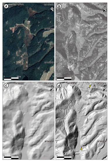
Figure 3.
Resolution comparison of various remote sensing technologies for the same area. (a) Google Earth Pro satellite image. (b) Aerial photography (1970s). (c) Hillshade using 1:5000 digital topographic maps (5 m resolution). (d) High-resolution LiDAR image hillshade. The yellow arrow indicates a fault scarp which was not observed in other images (0.5 m resolution).
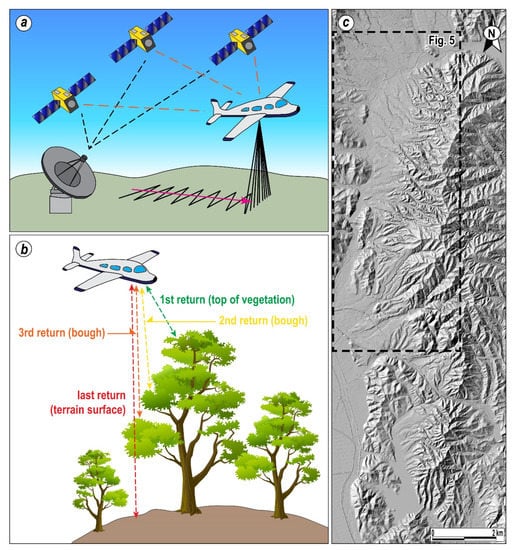
Figure 4.
Schematic diagrams showing the LiDAR imaging principles. (a) Airborne LiDAR imaging systems. (b) Laser point 3D surface information. (c) Airborne LiDAR imaging hillshade.
3.2. Electrical Resistivity & Trench Survey for Site Selection
An electrical resistivity survey is a geophysical technique used to recognize underground structures such as faults and rock boundaries. Electrical resistivity tomography (ERT) measures the potential differences in underground structures using a pair of electrodes to measure the difference in electrical resistivity which is then observed by interpreting the resultant 2D cross-section image. The electrical resistivity of rocks is determined based on the type of rock, porosity, permeability, and geological structures such as faults and joints [89]. When compared with ground penetrative radar (GPR), the ERT method has a deeper depth range and is able to distinguish the groundwater table. However, its limitation is that it is greatly affected by surface and underground conductive material. It is most commonly used in fault detection worldwide and is favored in Korea because the biophysical conditions presented by undulating forests and cultivated fields such as rice fields are not favorable for other geophysical techniques [38]. In this study, the AGI Mini Sting was used to perform the ERT along a lateral line of 150–200 m, with an electrode spacing of 10 m, and a depth of 50 m. Measurement data were processed into 2D images by inverse resistivity modeling using finite difference method (FDM) or finite element method (FEM) techniques, and geological structure and ground characteristics were expressed as high or low resistivity anomalies. The trench site was selected by precisely locating the fault using the analyzed ERT profile.
4. Results
4.1. Topographic Mapping Using High-Resolution LiDAR Data DEMs
The overall topography of the study area is divided into a lowland area in the west and a mountainous area in the east (Figure 5). The ridges of the western hills show irregular directions, but in the eastern mountains, the ridges extending from the summit are cut off by a lineament heading west. Most of the streams drain the high elevations in the east to the west, and several alluvial fans, fed from the sediments of the eastern mountains, are present at the foot slopes. We identified twelve lineaments in the study area through lineament analysis. The main lineament of high activity extends for 7.6 km passing through the northern side of the Byoekgye site. Two subsidiary lineaments of high activity are evident to the west of the 3.5–6.0 km section of the main lineament. The high activity lineament in the NNE direction also branches off the main lineament at 5.5 km. Low activity lineaments are primarily present in the N–S or NNE direction, which is the same direction as the high activity lineaments; however, most appear to be valleys eroded by fluvial and hillslope processes, rather than fault valleys. The main lineament is the longest and comprises continuous fault scarps and deflected streams. Most reservoirs are characteristically located along the main lineament, which also cuts alluvial fans. The impermeable fault gouges provide the water storage capability to the main lineament.
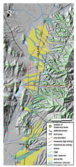
Figure 5.
Geomorphic mapping results of the study area using LiDAR imaging. The fault scarp is recognized along a main lineament extending northward from the previous studies sites (i.e., Byeokgye and Dangu). The study area is divided into two areas for detailed analysis. Each fault scarp is differentiated from other fluvial and man-made scarps by on-field confirmation considering its linear continuity and near-by connectivity using the different years of aerial photographs and topomaps.
We conducted a detailed topographic analysis by dividing the study area into south and north, centering on the main lineament. Fault scarps are continuously and distinctly visible in the main lineament of the southern section (Figure 6a). In the cross-section, the fault scarps are recognized as knickpoints, and on the topographical map, the ridges on the east side of the lineament are cut by the fault and merged with the alluvial fans (Figure 6b). In addition, fault scarps can be intuitively observed with the naked eye on the 3D view of the LiDAR data hillshade image (Figure 6c). The main lineament is located along the small valley floor between the hills and alluvial fans, therefore there is a high possibility that the Quaternary sedimentary deposits distributed in the lowlands may have traces of displacement or deformation created by a faulting event. Relatively large floodplains and fans are present in the southern section, ~300 m from the Byeokgye site; however, the fault landforms cannot be identified owing to the presence of agricultural land and river embankment construction.
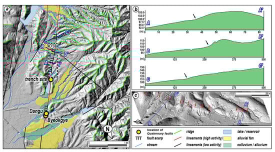
Figure 6.
(a) Detailed topographic map of the southern area. (b) Topographic profiles of the fault line (blue line in (a)) across the fault scarps. Black arrows point to knickpoints identified as fault scarps. (c) Hillshade image 3D view. The red arrows indicate the fault scarp, which is clearly visible to the naked eye.
The main lineament of the northern section is identified as a linear arrangement of deflected streams and fault scarps (Figure 7a). Unlike in the south, the fault scarps in the north show surface uplift estimated at a vertical offset of between 2–4.2 m of the same alluvial fan surface cross-section (Figure 7b). The 3D view of the hillshade image displays weak fault scarps in the southern section; however, they are visible to the naked eye (Figure 7c). On the western side of the main lineament, high activity lineaments with a vertical offset of 3–7.5 m developing into an en-echelon array are present (Figure 7a,b), and an NNE-striking high activity lineament with deflected streams with a dextral offset is present on the eastern side (Figure 7a). The horizontal offsets calculated based on the three deflected streams are 92 m, 98 m, and 150 m. The tendency for the offset to decrease as the distance from the main lineament increases indicates that the fault offset branching from the main fault gradually decreases.
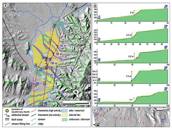
Figure 7.
(a) Detailed topographic map of the northern area. An NNE lineament branching from the main lineament is indicated by the dextrally deflected stream. (b) Topographic profiles of the line (blue line in (a)) across the fault scarps. Fault scarps in the northern section are evident based on the surface elevation difference in the similar landform. (c) Hillshade image 3D view. Red arrows indicate the fault scarp.
4.2. Electrical Resistivity and Trench Survey
4.2.1. Electrical Resistivity Survey
The electrical resistivity survey of the trench site was performed at a length of 200 m, electrode spacing of 10 m, and depth of 50 m. The measured resistivity values ranged from 16.6–502.5 Ω·m (Figure 8). The granite on the western side displayed a relatively high resistivity value compared to the sedimentary rock on the eastern side, and the low resistivity anomaly observed at the point was presumed to be the boundary extending to the surface (Figure 8b). The low resistivity anomaly of the surface is located between 105–120 m of the survey line, which is consistent with the lineament estimated from the fault scarp. The trench survey was conducted where the topographic analysis and electrical resistivity survey coincided.
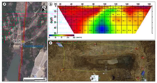
Figure 8.
(a) Location of the electrical resistivity survey line (black line) and trench site (square). The red line and blue circle indicate the main lineament and a low resistivity anomaly zone, respectively. (b) Electrical resistivity tomography (ERT) result. The blue zone, between 105–120 m, was selected as the trench site because of its low resistivity extending to the surface. (c) Trench site plan view.
4.2.2. Quaternary Fault Characteristics in the Trench
The trench was aligned in an E–W direction, 10 m long, 2 m wide, and 3.5 m deep (Figure 8c). In the trench section, seven fault surfaces (F1–F7) were observed dipping to the east either cutting the Quaternary sedimentary deposits or forming a boundary between the Quaternary sedimentary deposits and the pre-existing fault core (Figure 9). Based on the F6 fault surface, the hanging wall on the eastern side comprises a pre-existing fault core with a minimum width of 2.5 m, which may have formed before the Quaternary, while the footwall on the western side comprises the Quaternary sedimentary deposits. The fault core observed in the hanging wall is divided, with fault core 1 comprising a blue gouge, with a width of ~40 cm, cutting the Quaternary sediments, and a weakly developed shear band due to the arrangement of clay minerals. To the east of fault core 1, brown and gray fault core 2 has a width exceeding 2 m but does not cut the Quaternary sediments. Fault core 2 comprises a gouge zone containing a great deal of fault breccia with white, light gray, and dark gray gouge layers with a width of ~1 to 2 cm alternately present. In addition, the slickenline, which indicates the dextral strike-slip, is present on the slip surface between the fault breccia zone and the fault gouge. The Quaternary sedimentary deposits of the footwall have been subdivided into units (A to I from the top layer) based on grain size, type of clast and matrix, texture, roundness, sorting, and color, among others (Figure 10). The basement rock, A-type alkali granite, was observed below unit I. Unit A, included as a lens-shape in unit B, is a fine brown sandy silt that does not contain clast, whereas unit B, which is the thickest section, comprises dark brown cobble deposits containing various size breccias. Unit B becomes finer upward, and the clast size becomes smaller toward the surface. Unit C covering the hanging-wall side fault core of the F6 fault surface is a brown sand with cobble, which is a lighter color and shows better sorting and roundness compared to unit B and becoming thinner toward the west from the footwall and pinches out. Unit D is a light brown sand with pebble deposits, and although it is next to the fault the clast sorting and roundness are even. Since both boundaries of unit D are against a fault surface, it is highly probable that the nearby sediments were captured along the shear surface by horizontal displacement. Unit E comprises alternating fine gray sand and medium brown sand and various types of seismic soft-sediment deformation structures (SSDS) were also observed (Figure 10). The load structure, such as load casts, ball-and-pillow structure, and the intrusive structure such as flame structure, pillar structure, clastic dyke, disturbed structure, and structureless sediments were observed as SSDS. The intrusion structure is mainly observed in unit E (Figure 10a,b), and the load structure in unit G (Figure 10c). These structures were formed because of the liquefaction or fluidization of sediments due to seismic ground motion [90,91,92,93]. Unit F is grayish-white medium sand with 1–5 cm of felsic and granitic clasts and displays poor lateral continuity and sorting. Unit G is fine gray sand with granules and the load structure, which is an SSDS, is also well observed. Unit H is a brown gravelly fine sand, with a moderate roundness and sorting. Unit I, comprising A-type alkali feldspar granite, is a grayish-white gravelly fine sand and predominantly comprises felsic and granitic clasts, with a clast size ranging from 5–30 cm, with the clast appearance being similar to granite. The strike of the seven fault surfaces varies from N60°W to N28°E, and its dip-direction displays a change from NW to NNE as it continues eastward. The F6 fault surface (N01°E, 69°SE), which cuts up to unit B, the youngest unit among the Quaternary deposits, has a strike like the N–S lineament, which was confirmed by the LiDAR-driven DEM image. In contrast, F7 cuts up to unit C of the hanging wall, F3–F5 cut up to units D, E, and F, respectively, and are covered by unit C, whereas F1and F2 cut unit G but are covered by unit F. The slickenline is observed in the F6 fault surface, showing a dextral strike-slip with a rake of 30°N (Figure 10d). The OSL age of unit B cut by the F6 fault surface is 3200 ± 200 years [94,95], and the most recent earthquake fault is approximately after 3200 ± 200 years old.
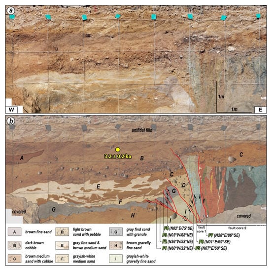
Figure 9.
(a) Trench site photomosaic. (b) Trench sketch. Seven fault surfaces (red line) and nine deposit units are evident in the section. Division of unit B by the most recent faulting event (3200 ± 200 year).
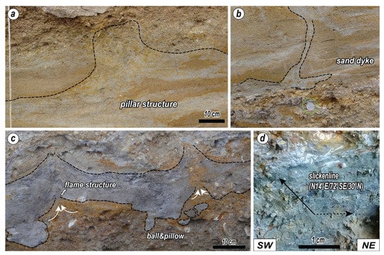
Figure 10.
Photograph showing features in a section of the trench. (a) Pillar structure and (b) sand dyke in unit E. (c) Flame and ball and pillow structures in unit G. (d) Slickenline on the F6 fault surface indicating dextral reverse faulting.
5. Conclusions
We identified the main lineament on the central Yangsan Fault, a major tectonic line in the Korean Peninsula by performing detailed topographic analysis using high-resolution LiDAR data. After identifying the lineament as a high activity seismic area as indicated by the topographic analysis, we conducted an electrical resistivity survey in the area to select a trench site. Finally, we identified an active fault in the trenched outcrop. The most recent earthquake occurred during the Holocene. In conclusion, we traced an active fault with high accuracy using LiDAR.
Korea, being located on an intraplate, has a relatively slow slip rate and seismic activity compared to countries located on plate boundaries. However, the recent medium-scale earthquakes that occurred in 2016 and 2017 drew much attention to the risk of seismic activity in Korea. Although research on active faults in Korea is limited compared to other countries, such as the United States, Japan, and Taiwan, the Korean government recently initiated a national active fault mapping program, resulting in an increase in the pace and amount of paleoseismological studies being undertaken. Owing to natural (e.g., humid climate and the rapid rate of surface erosion) and cultural (e.g., rapid urbanization and historic and current cultivation) conditions, the search for active faults, which is the basis of the paleoseismological study, was challenging. However, large-scale faults pass through or by most metropolitan areas in Korea (e.g., the Chugaryeong Fault in Seoul where there is a population of ~20 million people). For this reason, earthquake disaster countermeasures are essential in the long term for people living in proximity to fault lines. The first step for this is to identify active faults and construct reliable paleoseismic datasets. In this study, we were the first to apply the LiDAR technique to trace a major active fault in Korea and our study may assist stakeholders as well as geologists in policy and planning decisions to mitigate earthquake risks by providing reliable paleoseismic data.
Author Contributions
Conceptualization, S.H., Y.B.S. and M.S.; methodology, Y.B.S.; investigation, S.H.; data curation, Y.B.S.; writing—original draft preparation, S.H.; writing—review and editing, Y.B.S. and M.S.; visualization, S.H.; supervision, M.S.; project administration, Y.B.S.; funding acquisition, M.S. All authors have read and agreed to the published version of the manuscript.
Funding
This research was supported by a grant (2022-MOIS62-001) of National Disaster Risk Analysis and Management Technology in Earthquake funded by Ministry of Interior and Safety (MOIS, Korea).
Data Availability Statement
Not applicable.
Acknowledgments
We thank the anonymous reviewers for helping improve the manuscript.
Conflicts of Interest
The authors declare no conflict of interest.
References
- Coburn, A.W.; Spence, R.J.S. Earthquake Protection, 2nd ed.; Wiley: Chichester, UK, 2002. [Google Scholar]
- Blaikie, P.; Cannon, T.; Davis, I.; Wisner, B. At Risk: Natural Hazards, People’s Vulnerability and Disasters, 2nd ed.; Routledge: London, UK, 2004; p. 496. [Google Scholar]
- Stein, S.; Wysession, M. An Introduction to Seismology, Earthquakes, and Earth Structure; Blackwell Scientific: Malden, MA, USA, 2003. [Google Scholar]
- McCalpin, J.P. Chapter 9: Application of Paleoseismic Data to Seismic Hazard Assessment and Neotectonic Research. In Paleoseismology, 2nd ed.; International Geophysics Series; McCalpin, J.P., Ed.; Academic Press-Elsevier: Burlington, NJ, USA, 2009; Volume 95, pp. 1–106. [Google Scholar]
- Gurpinar, A. The importance of paleoseismology in seismic hazard studies for critical facilities. Tectonophysics 2005, 408, 23–28. [Google Scholar] [CrossRef]
- Reiter, L. Earthquake Hazard Analysis: Issue and Insights; Columbia University Press: New York, NY, USA, 1990; p. 254. [Google Scholar]
- McCalpin, J.P.; Nelson, A.R. Chapter 1: Introduction to paleoseismology. In Paleoseismology, 2nd ed.; International Geophysics Series; McCalpin, J.P., Ed.; Academic Press-Elsevier: Burlington, NJ, USA, 2009; Volume 95, pp. 1–27. [Google Scholar]
- Crone, A.J.; Omdahl, E.M. Directions in Paleoseismology. In U.S. Geological Survey Open-File Report; USGS: Denver, CO, USA, 1987; pp. 87–673. [Google Scholar]
- Yeats, R.S.; Prentice, C.S. Introduction to special section: Paleoseismology. J. Geophys. Res. 1996, 101, 5847–5853. [Google Scholar] [CrossRef]
- McCalpin, J.P. Chapter 2A: Field Techniques in Paleoseismology-Terrestrial Environments. In Paleoseismology, 2nd ed.; International Geophysics Series; McCalpin, J.P., Ed.; Academic Press-Elsevier: Burlington, NJ, USA, 2009; Volume 95, pp. 29–118. [Google Scholar]
- Goldfinger, C. Chapter 2B: Sub-Aqueous Paleoseismology. In Paleoseismology, 2nd ed.; McCalpin, J.P., Ed.; International Geophysics Series; Academic Press-Elsevier: Burlington, NJ, USA, 2009; Volume 95, pp. 119–170. [Google Scholar]
- Ganas, A.; Pavlides, S.; Karastathis, V. DEM-based morphometry of range-front escarpments in Attica, central Greece, and its relation to fault slip rates. Geomorphology 2005, 65, 301–319. [Google Scholar] [CrossRef]
- Oguchi, T.; Aoki, T.; Matsuta, N. Identification of an active fault in the Japanese Alps from DEM-based hill shading. Comput. Geosci. 2003, 29, 885–891. [Google Scholar] [CrossRef]
- Yang, Y.; Qin, X.; Shi, W.; Zhang, Y.; Zhao, Z. Segmentation of the active Liumugao Fault, NE Tibetan Plateau as revealed by DEM-derived geomorphic indices. Geosyst. Geoenviron. 2022, 1, 100056. [Google Scholar] [CrossRef]
- Viveen, W.; Baby, P.; Hurtado-Enríquez, C. Assessing the accuracy of combined DEM-based lineament mapping and the normalised SL-index as a tool for active fault mapping. Tectonophysics 2021, 813, 228942. [Google Scholar] [CrossRef]
- Wisely, B.A.; Schmidt, D. Deciphering vertical deformation and poroelastic parameters in a tectonically active fault-bound aquifer using InSAR and well level data, San Bernardino basin, California. Geophys. J. Int. 2010, 181, 1185–1200. [Google Scholar] [CrossRef]
- Xu, W.; Dutta, R.; Jónsson, S. Identifying Active Faults by Improving Earthquake Locations with InSAR Data and Bayesian Estimation: The 2004 Tabuk (Saudi Arabia) Earthquake Sequence. Bull. Seismol. Soc. Am. 2015, 105, 765–775. [Google Scholar] [CrossRef]
- Yao, X.; Li, L.; Zhang, Y.; Zhou, Z.; Liu, X. Types and characteristics of slow-moving slope geo-hazards recognized by TS-InSAR along Xianshuihe active fault in the eastern Tibet Plateau. Nat. Hazards 2017, 88, 1727–1740. [Google Scholar] [CrossRef]
- Ghayournajarkar, N.; Fukushima, Y. Determination of the dipping direction of a blind reverse fault from InSAR: Case study on the 2017 Sefid Sang earthquake, northeastern Iran. Earth Planets Space 2020, 72, 64. [Google Scholar] [CrossRef]
- Wang, Z.; Lawrence, J.; Ghail, R.; Mason, P.; Carpenter, A.; Agar, S.; Morgan, T. Characterizing Micro-Displacements on Active Faults in the Gobi Desert with Time-Series InSAR. Appl. Sci. 2022, 12, 4222. [Google Scholar] [CrossRef]
- Wang, H.; Wright, T.J.; Liu-Zeng, J.; Peng, L. Strain rate distribution in south-central Tibet from two decades of InSAR and GPS. Geophys. Res. Lett. 2019, 46, 5170–5179. [Google Scholar] [CrossRef]
- Zhao, D.; Qu, C.; Shan, X.; Gong, W.; Zhang, Y.; Zhang, G. InSAR and GPS derived coseismic deformation and fault model of the 2017 Ms7.0 Jiuzhaigou earthquake in the Northeast Bayanhar block. Tectonophysics 2018, 726, 86–99. [Google Scholar] [CrossRef]
- Chan, Y.-C.; Chen, Y.-G.; Shih, T.-Y.; Huang, C. Characterizing the Hsincheng active fault in northern Taiwan using airborne LiDAR data: Detailed geomorphic features and their structural implications. J. Asian Earth Sci. 2007, 31, 303–316. [Google Scholar] [CrossRef]
- Chen, T.; Zhang, P.Z.; Liu, J.; Li, C.Y.; Ren, Z.K.; Hudnut, K.W. Quantitative study of tectonic geomorphology along Haiyuan fault based on airborne LiDAR. Chin. Sci. Bull. 2014, 59, 2396–2409. [Google Scholar] [CrossRef]
- Hunter, L.E.; Howle, J.F.; Rose, R.S.; Bawden, G.W. LiDAR-Assisted Identification of an Active Fault near Truckee, California. Bull. Seismol. Soc. Am. 2011, 101, 1162–1181. [Google Scholar] [CrossRef]
- Cunningham, D.; Grebby, S.; Tansey, K.; Gosar, A.; Kastelic, V. Application of airborne LiDAR to mapping seismogenic faults in forested mountainous terrain, southeastern Alps, Slovenia. Geophys. Res. Lett. 2006, 33, L20308. [Google Scholar] [CrossRef]
- Chen, R.-F.; Lin, C.-W.; Chen, Y.-H.; He, T.-C.; Fei, L.-Y. Detecting and Characterizing Active Thrust Fault and Deep-Seated Landslides in Dense Forest Areas of Southern Taiwan Using Airborne LiDAR DEM. Remote Sens. 2015, 7, 15443–15466. [Google Scholar] [CrossRef]
- Prentice, C.S.; Crosby, C.J.; Whitehill, C.S.; Arrowsmith, J.R.; Furlong, K.P.; Phillips, D.A. Illuminating Northern California’s Active Faults. Eos Trans. AGU 2009, 90, 55. [Google Scholar] [CrossRef]
- Lin, Z.; Heitaro, K.; Sakae, M.; Norichika, A.; Tatsuro, C. Detection of subtle tectonic–geomorphic features in densely forested mountains by very high-resolution airborne LiDAR survey. Geomorphology 2013, 182, 104–115. [Google Scholar] [CrossRef]
- Moulin, A.; Benedetti, L.; Gosar, A.; Rupnik, P.J.; Rizza, M.; Bourlès, D.; Ritz, J.F. Determining the present-day kinematics of the Idrija fault (Slovenia) from airborne LiDAR topography. Tectonophysics 2014, 628, 188–205. [Google Scholar] [CrossRef]
- Scott, C.P.; DeLong, S.B.; Arrowsmith, J.R. Distribution of aseismic deformation along the Central San Andreas and Calaveras faults from differencing repeat airborne lidar. Geophys. Res. Lett. 2020, 47, e2020GL090628. [Google Scholar] [CrossRef]
- Marco, S.; Rockwell, T.K.; Heimann, A.; Frieslander, U.; Agnon, A. Late Holocene activity of the Dead Sea Transform revealed in 3D palaeoseismic trenches on the Jordan Gorge segment. Earth Planet Sci. Lett. 2005, 234, 189–205. [Google Scholar] [CrossRef]
- Medina-Cascales, I.; Koch, L.; Cardozo, N.; Martin-Rojas, I.; Alfaro, P.; García-Tortosa, F.J. 3D geometry and architecture of a normal fault zone in poorly lithified sediments: A trench study on a strand of the Baza Fault, central Betic Cordillera, south Spain. J. Struct. Geol. 2019, 121, 25–45. [Google Scholar] [CrossRef]
- Galli, P.A.C.; Giaccio, B.; Messina, P.; Peronace, E.; Zuppi, G.M. Palaeoseismology of the L’Aquila faults (central Italy, 2009, Mw 6.3 earthquake): Implications for active fault linkage. Geophys. J. Int. 2011, 187, 1119–1134. [Google Scholar] [CrossRef]
- Ferrater, M.; Echeverria, A.; Masana, E.; Martínez-Díaz, J.J.; Sharp, W.D. A 3D measurement of the offset in paleoseismological studies. Comput. Geosci. 2016, 90, 156–163. [Google Scholar] [CrossRef]
- Woo, J.-U.; Rhie, J.; Kim, S.; Kang, T.-S.; Kim, K.-H.; Kim, Y. The 2016 Gyeongju earthquake sequence revisited: Aftershock interactions within a complex fault system. Geophys. J. Int. 2019, 217, 58–74. [Google Scholar] [CrossRef]
- Kim, K.-H.; Ree, J.-H.; Kim, Y.; Kim, S.; Kang, S.Y.; Seo, W. Assessing whether the 2017 Mw 5.4 Pohang earthquake in South Korea was an induced event. Science 2018, 360, 1007–1009. [Google Scholar] [CrossRef]
- Kim, Y.-S.; Jin, K.; Choi, W.-H.; Kee, W.-S. Understanding of active faults: A review for recent researches. J. Geol. Soc. Korea 2011, 47, 723–752, (In Korean with English Abstract). [Google Scholar]
- Lee, K.; Na, S.H. A study of microearthquake activity of the Yangsan fault. J. Geol. Soc. Korea 1983, 19, 127–135, (In Korean with English Abstract). [Google Scholar]
- Okada, A.; Watanabe, M.; Sato, H.; Jun, M.S.; Jo, W.R.; Kim, S.K.; Jeon, J.S.; Chi, H.C.; Oike, K. Active fault topography and trench survey in the central part of the Yangsan fault, southeast Korea. J. Geogr. 1994, 103, 111–126, (In Japanese with English Abstract). [Google Scholar] [CrossRef]
- Korea Hydro & Nuclear Power Co. Ltd. Preliminary Safety Analysis Report of Shin KORI Units 3; Korea Hydro & Nuclear Power Co. Ltd.: Gyeongju-si, Korea, 2002; 133p. (In Korean) [Google Scholar]
- Korea Hydro & Nuclear Power Co. Ltd. Preliminary Safety Analysis Report of Shin WOLSUNG Units 1; Korea Hydro & Nuclear Power Co. Ltd.: Gyeongju-si, Korea, 2003; 574p. (In Korean) [Google Scholar]
- Lee, K.; Lee, J.; Kyung, J.B. A Statistical analysis of the seismicity of the Yangsan Fault System. J. Eng. Geol. 1998, 8, 99–114, (In Korean with English Abstract). [Google Scholar]
- Chwae, U.; Lee, D.Y.; Lee, B.J.; Ryoo, C.-R.; Choi, P.-Y.; Choi, S.-J.; Cho, D.-L.; Kim, J.-Y.; Lee, C.B.; Kee, W.S.; et al. An Investigation and Evaluation of Capable Fault: Southeastern Part of the Korean Peninsula; KIGAM: Daejeon, Korea, 1998; p. 324. (In Korean) [Google Scholar]
- Kyung, J.B. Paleoseismological study on the mid-northern part of Ulsan fault by trench method. J. Eng. Geol. 1997, 7, 81–90, (In Korean with English Abstract). [Google Scholar]
- Kyung, J.B.; Lee, K.; Okada, A. A paleoseismological study of the Yangsan fault-Anaysis of deformed topography and trench survey. J. Korean Geophys. Soc. 1999, 2, 155–168, (In Korean with English Abstract). [Google Scholar]
- Kyung, J.B.; Lee, K.; Okada, A.; Watanabe, M.; Suzuki, Y.; Takemura, K. Study of fault characteristics by trench survey in the Sangchon-ri area in the southern part of Yangsan fault, southeastern Korea. J. Korean Earth Sci. Soc. 1999, 20, 101–110, (In Korean with English Abstract). [Google Scholar]
- Kee, W.-S.; Kim, B.C.; Hwang, J.H.; Song, K.-Y.; Kihm, Y.-H. Structural Characteristics of Quaternary reverse faulting on the Eupcheon Fault, SE Korea. J. Geol. Soc. Korea 2007, 43, 311–333, (In Korean with English Abstract). [Google Scholar]
- Kim, Y.-S.; Kihm, J.-H.; Jin, K. Interpretation of the rupture history of a low slip-rate active fault by analysis of progressive displacement accumulation: An example from the Quaternary Eupcheon Fault, SE Korea. J. Geol. Soc. 2011, 168, 273–288. [Google Scholar] [CrossRef]
- Zonenshain, L.P.; Savostin, L.A. Geodynamics of the Baikal rift zone and plate tectonics of Asia. Tectonophysics 1981, 76, 1–45. [Google Scholar] [CrossRef]
- Minster, J.B.; Jordan, T.H. Present-day plate motions. J. Geophys. Res. 1978, 83, 5331–5354. [Google Scholar] [CrossRef]
- DeMets, C.; Gordon, R.G.; Argus, D.F.; Stein, S. Current plate motions. Geophys. J. Int. 1990, 101, 425–478. [Google Scholar] [CrossRef]
- DeMets, C.; Gordon, R.G.; Argus, D.F.; Stein, S. Effect of recent revisions to the geomagnetic reversal time scale on estimates of current plate motions. Geophys. Res. Lett. 1994, 21, 2191–2194. [Google Scholar] [CrossRef]
- Bird, P. An updated digital model of plate boundaries. Geochem. Geophys. Geosyst. 2003, 4, 1027. [Google Scholar] [CrossRef]
- Korea Meteorological Administration. Available online: https://www.weather.go.kr/w/eqk-vol/archive/stat/trend.do (accessed on 16 March 2022). (In Korean).
- Lee, K. Historical earthquake data of Korean. J. Korea Geophys. Soc. 1998, 1, 3–22, (In Korean with English Abstract). [Google Scholar]
- Lee, K.; Yang, W.-S. Historical Seismicity of Korea. Bull. Seismol. Soc. Am. 2006, 96, 846–855. [Google Scholar] [CrossRef]
- Kim, K.-H.; Kang, T.-S.; Rhie, J.; Kim, Y.H.; Park, Y.; Kang, S.Y.; Han, M.; Kim, J.; Park, J.; Kim, M.; et al. The 12 September 2016 Gyeongju earthquakes: 2. Temporary seismic network for monitoring aftershocks. Geosci. J. 2016, 20, 753–757. [Google Scholar] [CrossRef]
- Kim, K.-H.; Seo, W.; Hang, J.; Kwon, J.; Kang, S.Y.; Ree, J.-H.; Kim, S.; Liu, K. The 2017 ML 5.4 Pohang earthquake sequence, Korea, recorded by a dense seismic network. Tectonophysics 2020, 774, 228306. [Google Scholar] [CrossRef]
- Han, M.; Kim, K.-H.; Son, M.; Kang, S.Y.; Park, J.-H. Location of recent micro earthquakes in the Gyeongju area. Geophys. Geophys. Explor. 2016, 19, 97–104, (In Korean with English Abstract). [Google Scholar] [CrossRef]
- Lee, J.; Ryoo, Y.; Park, S.C.; Ham, Y.M.; Park, J.S.; Kim, M.S.; Park, S.M.; Cho, H.G.; Lee, K.S.; Kim, I.S.; et al. Seismicity of the 2016 ML 5.8 Gyeongju earthquake and aftershocks in South Korea. Geosci. J. 2018, 22, 433–444. [Google Scholar] [CrossRef]
- Park, Y.; Ree, J.-H.; Yoo, S.-H. Fault slip analysis of Quaternary faults in southeastern Korea. Gondwana Res. 2006, 9, 118–125. [Google Scholar] [CrossRef]
- Kim, M.-C.; Jung, S.; Yoon, S.; Jeong, R.-Y.; Song, C.W.; Son, M. Neotectonic crustal deformation and current stress field in the Korean Peninsula and Their Tectonic Implications: A review. J. Petrol. Soc. Korea 2016, 25, 169–193, (In Korean with English Abstract). [Google Scholar] [CrossRef]
- Nahm, W.-H.; Lee, H.; Jun, C.-P. Holocene uplift rates in Korea. Korean J. Quat. Res. 2018, 32, 41–50. (In Korean) [Google Scholar]
- Lee, S.Y.; Seong, Y.B.; Choi, K.H.; Yu, B.Y. Cosmogenic 10Be and OSL dating of marine terraces along the central -east coast of Korea: Spatio-temporal variations in uplift rates. Open Geogr. J. 2015, 7, 28–39. [Google Scholar] [CrossRef][Green Version]
- Korea Meteorological Administration. In 2021 Year Book. Available online: https://www.kma.go.kr (accessed on 6 March 2022). (In Korean).
- Kee, W.-S.; Kim, Y.-H.; Lee, H.-J.; Choi, D.-L.; Kim, B.-C.; Song, K.-Y.; Koh, H.-J.; Lee, S.R.; Gwang, Y.Y.; Hwang, S.-H.; et al. South Eastern Fault Variable Research and DB Construction; KIGAM: Daejeon, Korea, 2009; 327p. (In Korean) [Google Scholar]
- Choi, S.-J.; Jeon, J.S.; Song, G.Y.; Kim, H.C.; Kim, Y.H.; Choi, B.Y.; Chwae, W.C.; Han, J.G.; Ryoo, C.R.; Seon, C.G.; et al. Active Fault Map and Seismic Hazard Map; NEMA: Seuol, Korea, 2012; 939p. (In Korean) [Google Scholar]
- Cheon, Y.; Choi, J.-H.; Kim, N.; Lee, H.; Choi, I.; Bae, H.; Rockwell, T.K.; Lee, S.R.; Ryoo, C.-R.; Choi, H. Late Quaternary transpressional earthquakes on a long-lived intraplate fault: A case study of the Southern Yangsan Fault, SE Korea. Quat. Int. 2020, 553, 132–143. [Google Scholar] [CrossRef]
- Cheon, Y.; Ha, S.; Lee, S.; Cho, H.; Son, M. Deformation features and history of the Yangsan Fault Zone in the Eonyang-Gyeongju area, SE Korea. J. Geol. Soc. Korea 2017, 53, 95–114, (In Korean with English Abstract). [Google Scholar] [CrossRef]
- Cheon, Y.; Cho, H.; Ha, S.; Kang, H.-C.; Kim, J.-S.; Son, M. Tectonically controlled multiple stages of deformation along the Yangsan Fault Zone, SE Korea, since Late Cretaceous. J. Asian Sci. 2019, 170, 188–207. [Google Scholar] [CrossRef]
- Cheon, Y.; Choi, J.-H.; Choi, Y.; Bae, H.; Han, K.-H.; Son, M.; Choi, S.-J.; Ryoo, C.-R. Understanding the distribution and internal structure of the main core of the Yangsan Fault Zone: Current trends and future work. J. Geol. Soc. Korea 2020, 56, 619–640, (In Korean with English Abstract). [Google Scholar] [CrossRef]
- Choi, J.-H.; Kim, Y.-S.; Klinger, Y. Recent progress in studies on the characteristics of surface rupture associated with large earthquakes. J. Geol. Soc. Korea 2017, 53, 129–157, (In Korean with English Abstract). [Google Scholar] [CrossRef]
- Chang, K.H.; Woo, B.G.; Lee, J.H.; Park, S.O.; Yao, A. Cretaceous and early Cenozoic stratigraphy and history of eastern Kyongsang Basin, S. Korea. J. Geol. Soc. Korea 1990, 26, 471–487. [Google Scholar]
- Hwang, B.H.; Lee, J.D.; Yang, K. Petrological study of the granitic rocks around the Yangsan fault: Lateral displacement of the Yangsan fault. J. Geol. Soc. Korea 2004, 40, 161–178, (In Korean with English Abstract). [Google Scholar]
- Hwang, B.H.; Lee, J.D.; Yang, K.; McWilliams, M. Cenozoic strike-slip displacement along the Yangsan fault, southeast Korean Peninsula. Int. Geol. Rev. 2007, 49, 768–775. [Google Scholar] [CrossRef]
- Hwang, B.H.; McWilliams, M.; Son, M.; Yang, K. Tectonic implication of A-type granites across the Yangsan fault, Gigye and Gyeongju areas, southeast Korean Peninsula. Int. Geol. Rev. 2007, 49, 1094–1102. [Google Scholar] [CrossRef]
- Ryoo, C.-R.; Lee, B.-J.; Cho, D.-L.; Chwae, U.-C.; Choi, S.-J.; Kim, J.-Y. Quaternary fault of Dangu-ri in Gyeongju Gangdong-myeon: Byeokgye fault. In Proceedings of the Korean Society of Economic and Environmental Geology/The Korean Society of Mineral and Energy Resources Engineers/Korean Society of Earth and Exploration Geophysicists, Spring Joint Conference, Chungnam National University, Daejeon, Korea, 14 April 1999; p. 334. [Google Scholar]
- Lee, J.; Rezaei, S.; Hong, Y.; Choi, J.-H.; Choi, J.-H.; Choi, W.-H.; Rhee, K.-W.; Kim, Y.-S. Quaternary fault analysis through a trench investigation on the northern extension of the Yangsan fault at Dangu-ri, Gyungju-si, Gyeongsangbuk-do. J. Geol. Soc. Korea 2015, 51, 471–485, (In Korean with English Abstract). [Google Scholar] [CrossRef]
- Hwang, J.H.; Kim, D.H.; Cho, D.R.; Song, K.Y. Explanatory Note of The Andong Sheet, 1:1:250,000; Korea Institute of Geoscience and Mineral Resources: Daejeon, Korea, 1996; 67p. (In Korean) [Google Scholar]
- Kim, D.H.; Hwang, J.H.; Park, K.H.; Song, K.Y. Explanatory Note of The Pusan Sheet, 1:1:250,000; Korea Institute of Energy and Resources: Daejeon, Korea, 1998; 62p. (In Korean) [Google Scholar]
- Son, M.; Song, C.W.; Kim, M.-C.; Cheon, Y.; Cho, H.; Sohn, Y.K. Miocene tectonic evolution of the basins and fault systems, SE Korea: Dextral, simple shear during the East Sea (Sea of Japan) opening. J. Geol. Soc. 2015, 172, 664–680. [Google Scholar] [CrossRef]
- Song, C.W. Study on the Evolution of the Miocene Pohang Basin Based on Its Structural Characteristics. Ph.D. Thesis, Pusan National University, Pusan, Korea, 2015; 146p. (In Korean with English Abstract). [Google Scholar]
- Kang, H.-C.; Cheon, Y.; Ha, S.; Seo, K.; Kim, J.-S.; Shin, H.C.; Son, M. Geology and U-Pb age in the eastern part of Yeongdeok-gun, Gyeongsangbuk-do, Korea. J. Petrol. Soc. Korea. 2018, 27, 153–171, (In Korean with English Abstract). [Google Scholar]
- Staley, D.M.; Wasklewicz, T.A.; Blaszczynski, J.S. Surficial patterns of debris flow deposition on alluvial fans in Death Valley, CA using airborne laser swath mapping data. Geomorphology 2006, 74, 152–163. [Google Scholar] [CrossRef]
- Volker, H.X.; Wasklewicz, T.A.; Ellis, M.A. A topographic fingerprint to distinguish alluvial fan formative processes. Geomorphology 2007, 88, 34–45. [Google Scholar] [CrossRef]
- Arrowsmith, J.R.; Zielke, O. Tectonic geomorphology of the San Andreas Fault zone from high resolution topography: An example from the Cholame segment. Geomorphology 2009, 113, 70–81. [Google Scholar] [CrossRef]
- Kondo, H.; Toda, S.; Okumura, K.; Takada, K.; Chiba, T. A fault scarp in an urban area identified by LiDAR survey: A Case study on the Itoigawa-Shizuoka Tectonic Line, central Japan. Geomorphology 2008, 101, 731–739. [Google Scholar] [CrossRef]
- Telford, W.M.; Geldart, P.L.; Sheriff, R.E. Applied Geophysics, 2nd ed.; Cambridge University Press: New York, NY, USA, 1990; 770p. [Google Scholar]
- Silva, P.G.; Rodríguez-Pascua, M.A.; Giner Robles, J.L.; Élez, J.; Pérez-López, R.; Davila, M.B.B. Catalogue of the Geological Effects of Earthquakes in Spain Based on the ESI-07 Macroseismic Scale: A New Database for Seismic Hazard Analysis. Geosciences 2019, 9, 334. [Google Scholar] [CrossRef]
- Martín-Chivelet, J.; Palma, R.M.; López-Gómez, J.; Kietzmann, D.A. Earthquake-induced soft-sediment deformation structures in Upper Jurassic open-marine microbialites (Neuquén Basin, Argentina). Sediment. Geol. 2011, 235, 210–221. [Google Scholar] [CrossRef]
- Owen, G.; Moretti, M. Identifying triggers for liquefaction-induced soft-sediment deformation in sands. Sediment. Geol. 2011, 235, 141–147. [Google Scholar] [CrossRef]
- Kang, H.-C.; Paik, I.S.; Lee, H.I.; Lee, J.E.; Chun, J.H. Soft-sediment deformation structures in Cretaceous non-marine deposits of southeastern Gyeongsang Basin, Korea: Occurrences and origin. Isl. Arc 2010, 19, 628–646. [Google Scholar] [CrossRef]
- Song, Y.; Ha, S.; Lee, S.; Kang, H.-C.; Choi, J.-H.; Son, M. Quaternary structural characteristics and paleoseismic interpretation of the Yangsan Fault at Dangu-ri, Gyeongju-si, SE Korea, through trench survey. J. Geol. Soc. Korea 2020, 56, 155–173, (In Korean with English Abstract). [Google Scholar] [CrossRef]
- Kim, S. Luminescence Dating of Active (Quaternary) Faults in the Southeastern Part of Korean Peninsula. Ph.D. Thesis, Pusan National University, Pusan, Korea, 2022; 146p. (In Korean with English Abstract). [Google Scholar]
Publisher’s Note: MDPI stays neutral with regard to jurisdictional claims in published maps and institutional affiliations. |
© 2022 by the authors. Licensee MDPI, Basel, Switzerland. This article is an open access article distributed under the terms and conditions of the Creative Commons Attribution (CC BY) license (https://creativecommons.org/licenses/by/4.0/).