Abstract
In recent decades, European countries have faced repeated heat waves. Traditionally, atmospheric CO2 concentration linked to repeated heat wave-induced photosynthetic inhibition has been explored based on local-specific in-situ observations. However, previous research based on field surveys has limitations in exploring area-wide atmospheric CO2 concentrations linked to repeated heat wave-induced photosynthetic inhibition. The present study aimed to evaluate the spatial cross-correlation of Greenhouse gases Observing SATellite (GOSAT) CO2 concentrations with repeated heat wave-induced photosynthetic inhibition in Europe from 2009 to 2017 by applying geographically weighted regression (GWR). The local standardized coefficient of a fraction of photosynthetically active radiation (FPAR: −0.24) and the normalized difference vegetation index (NDVI: −0.22) indicate that photosynthetic inhibition increases atmospheric CO2 in Europe. Furthermore, from 2009 to 2017, the heat waves in Europe contributed to CO2 emissions (27.2–32.1%) induced by photosynthetic inhibition. This study provides realistic evidence to justify repeated heat wave-induced photosynthetic inhibition as a fundamental factor in mitigating carbon emissions in Europe.
1. Introduction
The intensity and frequency of heat waves, described as periods of days with unprecedented high temperatures, have intensified during the last decade and are anticipated to increase in the 21st century [1]. Due to continuous record-breaking high temperatures, the heat waves have expanded in amplitude and spatial extent in Europe during recent decades [2]. For instance, temperature observation records at European stations continue to be broken every year [3]. In this regard, the length of heat waves in summer has increased twofold, and the number of days reporting heat extremes has increased threefold in Europe [4]. These heat wave events are projected to become more frequent and intense in Europe.
Plants respond to heat waves by adjusting their physiological structures, such as decreased leaf area, root–shoot ratio changes, or osmolyte concentration [5]. This causes decreased CO2 assimilation rates by reducing photosynthetic enzymes and sink strength and increasing source activity (respiration). It is thus necessary to elucidate the current status of CO2 emitted and absorbed according to photosynthetic inhibition and net primary productivity since heat waves are a crucial regulator of rising atmospheric CO2 concentrations [6].
It is essential to explore the vertical profile of CO2 that changes according to the photosynthetic action of vegetation and the use of fossil fuels as it is transported from the ground to the upper atmosphere. The mechanisms of greenhouse gases, including CO2, are monitored at approximately 530 ground stations operated by the World Meteorological Organization (WMO) [7]. However, these field-oriented surveys have considerable limitations in generalizing research outcomes because CO2 concentrations vary significantly in time and space, and the survey area is limited to the range of the WMO station.
Satellite-based XCO2 (column-averaged CO2) carries large amounts of information from the bottom atmospheric layer (near-ground) to the top of the atmosphere, including background atmospheric CO2 [8,9,10]. Hence, satellite-based XCO2 can be a valuable indicator of atmospheric CO2 caused by photosynthetic inhibition on a regional scale. Recently, the observation of CO2 through advanced remote sensing technology has been suggested to overcome the spatio-temporal limitations of existing measurements. The Greenhouse gases Observing SATellite (GOSAT) is the most advanced satellite system for observing CO2, and its usefulness has been recognized in various studies [11,12,13].
The relationship between photosynthetic inhibition induced by heat waves and its influence on the atmospheric CO2 growth rate varies regionally, annually, and seasonally with time (including day and night) [14]. Geographically weighted regression (GWR) provides a weighting of locally correlated information and allows the building of local regression model parameters varying in space during the last ten years. Hence, GWR could help to reveal spatiotemporal variations in the empirical relationships between photosynthetic inhibition and CO2 concentration over a more extended period. Previous studies have reported that heat waves affect the seasonal photosynthetic responses of European oak [15]. It was confirmed that these studies were the closest to the topic to be dealt with in this study. Therefore, this study aimed to evaluate the spatial cross-correlation of GOSAT CO2 concentrations with repeated heat wave-induced photosynthetic inhibition in Europe from 2009 to 2017.
2. Materials and Methods
2.1. Study Area
Europe is the second-smallest continent after Australia but includes 18 climate zones in small continents from Arid to Polar [16]. There are various types of plants in Europe, such as boreal tundra woodland, boreal coniferous forest, temperate steppe, temperate continental forest, subtropical dry forest, and so on [17]. The 18 climate zones show the different frequencies and characteristics of heat waves within the European continent. The diverse types of heat waves that occurred in the 18 climate zones induce photosynthetic inhibition stress in terms of diverse exposure temperatures, such as exposure duration, the ability of tolerance or acclimation, time of year, and soil moisture availability. The heat stress of terrestrial plants inhabited in 18 climates can present the quantitative influence of differentiated response patterns on photosynthetic inhibition (reductions of carbon assimilation and growth) [18]. Therefore, the European continent is ideal for studying heat wave-induced photosynthetic inhibitions from terrestrial plants.
2.2. Variables for Building the GWR Model
In this study, we utilized satellite observation data acquired by the Moderate Resolution Imaging Spectroradiometer (MODIS) onboard the Terra satellite from June 2009 to October 2017: normalized difference vegetation index (NDVI; MOD13A2), leaf area index (LAI), fraction of photosynthetically active radiation (FPAR; MOD15A2), daytime and nighttime land surface temperatures (LSTs; MOD11A2), and daily net photosynthesis (PSNet; MOD17a2) (Table 1). The original temporal and spatial resolutions of LAI, FPAR, and PSNet were eight days and 0.5 km; those of NDVI were 16 days and 1 km; and those of LST were eight days and 1 km, respectively. MODIS is a major observation sensor mounted on NASA’s Earth Observation Satellite, with multipurpose sensors that can be applied to the ocean, land, and atmosphere. The MODIS sensors observe the Earth’s surface once or twice a day at an altitude of 705 km, with a viewing angle of ±55°, an observation width of 2330 km, and a total of thirty-six spectral bands in the range of 0.4–14.4 μm. Two of the bands make 250-m resolution images at the nadir, five bands have a resolution of 500 m, and the remaining 29 bands have a resolution of 1 km.

Table 1.
Descriptive statistics for monthly anomalies of dependent and independent variables used in GWR.
The GOSAT Level 4 (L4) product comprises Level 4A (L4A) surface CO2 flux data and Level 4B (L4B) 3D-CO2 concentrations modeled with L4A. The L4B data contain the CO2 concentrations at 17 vertical levels from the ground to the upper atmosphere (666 km) [19]. The closest vertical level of the L4B data to the ground is 975 hPa [20]. Because the CO2 nearest to the ground surface provides more information on changes in the CO2 sink and source, this study utilized the L4B CO2 concentrations at 975 hPa to reflect near-ground CO2. The L4B product for CO2 was obtained between June 2009 and October 2017. The GOSAT L4B data provide the average monthly CO2 concentrations modeled on a 2.5° × 2.5° horizontal grid in netCDF format. Therefore, we fitted the spatial and temporal scales of the MODIS indicators into GOSAT XCO2 by averaging MODIS observations. This study used the monthly anomalies of GOSAT XCO2 and MODIS observations to build the GWR model.
2.3. Moran’s I Analysis
When analyzing the statistical distribution of spatial data, the results differ according to the location and circumstances of the data. This is because spatial data are related to each other due to the influence of spatial interaction and spatial diffusion. Before performing the spatial regression, spatial autocorrelation tests were conducted for each explanatory and dependent variable. Spatial autocorrelation is multidimensional (i.e., two to three dimensions of space) and multidirectional; it is more complicated than one-dimensional autocorrelation. The GWR builds a regional regression model using spatial weights. Therefore, spatial autocorrelation must be investigated before building the GWR model. Hence, we utilized Moran’s I to evaluate the autocorrelations of the variables used to build the GWR model.
Moran’s I was computed from −1 to 1. The negative autocorrelation (close to −1) exhibits that nearby locations tend to have unrelated values in adjacent areas [10]. By contrast, a positive autocorrelation (close to 1) implies that similar values tend to occur in adjacent areas. The spatial arrangement is randomly distributed if there is no spatial autocorrelation (close to zero). In this study, individual variables for GWR showed strong positive autocorrelations of 0.61–0.86 (Table 2). The mean autocorrelation of GOSAT Level 4 XCO2 appears the highest at 0.86, while the average latent heat flux appears the lowest at 0.61. The autocorrelation of GOSAT Level 4 XCO2 is strongly associated with the spatial distribution of CO2 sources and sinks. The GOSAT Level 4 XCO2 is calculated with Priori flux, which utilizes ODIAC data. ODIAC data is a global, high-resolution monthly emission data, which disaggregates the emission from diverse CO2 sources (fossil fuel, nuclear, hydro, and other renewable energy plants) obtained from the Carbon Monitoring for Action (CARMA) data set [21]. Average latent heat flux is estimated with diverse data such as land surface temperature (LST), the fraction of absorbed photosynthetically active radiation (FPAR), the normalized difference vegetation index (NDVI), the enhanced vegetation index (EVI), leaf area index (LAI), and albedo [22]. The parameters for estimating average latent heat flux are heterogeneous in the terrestrial landscape [23]. Thereby, it shows less autocorrelation than other indicators.
Table 2.
Descriptive statistics for Moran’s I estimated from individual variables.
2.4. Building GWR Model
A GWR local model was employed to evaluate how the variations in carbon uptake sources and GOSAT XCO2 regional relationships changed from 2009 to 2017. GWR is a local regression that locally differentiates the variables of a regression estimation. Unlike traditional regression, which establishes a single global regression among explanatory and response variables, GWR considers spatial variation in a model and provides maps to explain spatial non-stationarity [24,25]. The GWR is estimated by multiplying the geographically weighted matrix composed of geo-references [24,26]. is calibrated using the geographically neighboring spatial relations between points. In this study, we presumed that the degree of influence had an inverse ratio to the square distance of GOSAT Level 4. This means that the greater the is, the closer the points of geographical data and the stronger their influence on one another [27]. This study examined the spatial variability of a locally computed coefficient to identify the underlying process that presents spatial heterogeneity [24]. The regression model can be defined as follows (Equation (1)):
where represents the parameters estimated at each independent variable in which the coordinates are presented by vector . denotes the regression coefficient for the ith datum of independent variables (LST, NDVI, FPAR, LAI, Average latent heat flux, emission). is a residual [28]. Our analysis was implemented utilizing ArcMap 10.3 with a significance level of 0.05. Because the distribution of variables in the study area was non-uniform, an adaptive kernel was selected.
2.5. Mediation Analysis
Mediation analysis helps interpret the causality between dependent and independent variables by adding a third mediator, as there is a hidden connection between these variables [29]. Baron and Kenny (1986) found that four criteria have to be satisfied to implement the mediation analysis [30], as shown below (Table 3); (1) significantly accounting for , (2) significantly accounting for , (3) significantly accounting for , (4) decreases in the effect of on with entered simultaneously with . Table 3 presents the evidence that the results of this study satisfy the four criteria suggested by Baron and Kenny (1986) [30]. Based on this result, we assume that LST () directly or indirectly involves the changes in the effects of photosynthetic activities (), preceding changes in GOSAT XCO2 (). The total effects of MODIS photosynthetic indicators on GOSAT XCO2 could be apportioned individually into direct and indirect effects from an LST (mediator). Preacher and Hayes bootstrapping [31] with 5000 bootstrap samples were utilized to investigate mediation effects that can be caused by LSTs.
Table 3.
Results of Pearson’s r among mediator (LST), independent (NDVI, FPAR, LAI) and dependent variables (GOSAT Level4 XCO2).
3. Results
Figure 1 and Table 4 present the results of the 10-year GWR with the monthly anomaly of GOSAT level 4 XCO2 versus photosynthetic activity. NDVI, FPAR, and LAI have negative mean values of the standardized local coefficient of −0.22, −0.24, and −0.16, respectively. A decrease in chlorophyll levels affects the ability of plants to reflect incident solar radiation. Hence, stressed plants with low photosynthetic capability have reduced NDVI values. The distribution of LAI is another crucial determinant of photosynthesis because canopy leaf area rather than vegetation cover indicated by NDVI is often chosen as a base reference for the growth index of plants [32,33,34]. Therefore, the negative local coefficients of NDVI, FPAR, and LAI on GOSAT level 4 XCO2 show that the capability of photosynthetic activities in Europe has been reduced from 2009 to 2017. Changes in NDVI, FPAR and LAI possibly contributed to increasing atmospheric CO2 because of the reduced capability of photosynthetic activities in terrestrial ecosystems. Temperature showed the most decisive positive influence (0.35) on the geographical variations in CO2 concentrations during June 2009–October 2017. In this study, LST and latent heat flux increased sharply, whereas FPAR decreased. This has been caused by the scarcity of nutrients, humidity, and water stress due to the rapid increase in temperature and latent heat flux. This possibly has impeded the growth of carbon stocks through photosynthetic inhibition.
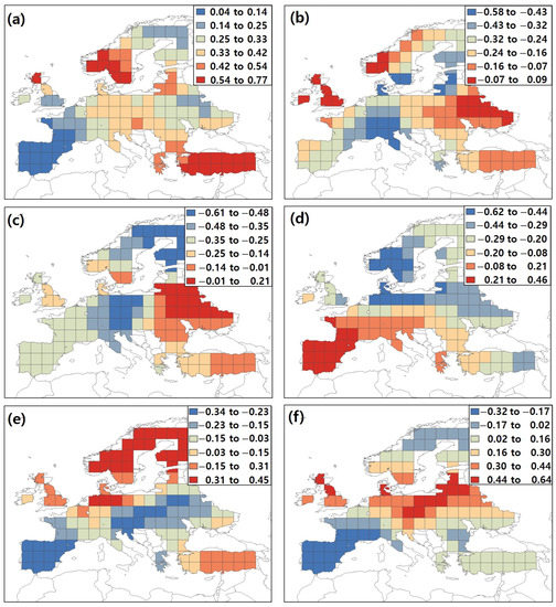
Figure 1.
Regional mean of GWR local coefficient. (a) Temperature. (b) NDVI. (c) Fraction of photosynthetically active radiation (FPAR). (d) Leaf area index (LAI). (e) Average latent heat flux. (f) ODIAC-PSNet.
Table 4.
Results of the GWR between GOSAT XCO2 (dependent variables) and heat wave-induced photosynthetic factor, including CO2 emissions (ODIAC-PSnet, independent variables).
During one specific heat wave, the local R2 and R2 plunged simultaneously (Figure 2). It was the second hottest year without an El Niño since 1850 [35]. Heat stress causes reductions in enzymatic activity [36], mesophyll/chlorophyll, and stomatal conductance [37]. The structural changes that occurred by leaf wilting and rolling decreased NDVI and LAI, reducing FPAR [38]. However, according to Shekhar et al. (2020), FPAR from European forest areas during the heat wave and drought events was not lower than FPAR in the past three years. While FPAR did not decrease, the proportion of FPAR decreased in transporting electrons for carbon assimilation, causing a surplus of photosynthetic energy [39]. It is considered that a similar pattern has occurred in this study. In August 2013 (heat wave events happened), the NDVI and LAI were relatively low, but the FPAR was the highest in the study period (Figure 3). Generally, the relations between NDVI, LAI, and FPAR are positively linear [40]. This abnormal negative correlation between NDVI, LAI, and FPAR involves the stiff decline of R2 and local R2 in August 2013.
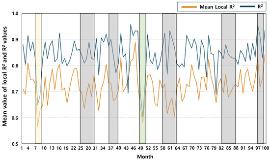
Figure 2.
Results of monthly mean local R2 and R2 values of GWR without the temporal bandwidth during June 2009–October 2017. The yellow box represents the coldest winter in Europe during 2009–2017. The green box represents August 2013, the second hottest year without an El Niño since 1850 [35]. Grey boxes indicate the months showing the largest discrepancy between local R2 and R2 during 2009–2017.
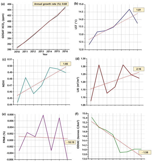
Figure 3.
Annual trends of GOSAT XCO2 and carbon uptake sources in Europe during 2010–2016. Red dotted lines are the trend lines used with the linear fit (x-axis: year). The years 2009 and 2017 are not presented in Figure 3 due to the lack of data for calculating the annual mean values. (a) GOSAT XCO2. (b) LST. (c) NDVI. (d) LAI. (e) FPAR. (f) Open-source Data Inventory for Anthropogenic CO2 (ODIAC).
The indirect effects of sudden climatic events (higher heating demands, drought, etc.) have influenced terrestrial carbon uptake activities, leading to decreased local R2 and R2. According to Bezak and Mikoš (2020) [41], heat waves have shown an increased probability of occurrence with compound events (hot and dry) across Europe during recent decades. Moreover, the heat waves with high surface temperature tend to cause the soil moisture deficit reducing the evaporative cooling and increasing heat flux. In turn, this exacerbates the prevailing drought condition in Europe [42]. Therefore, Europe’s photosynthetic inhibition resulted from heat waves and coincident droughts.
Interestingly, as we explored the monthly local R2 and R2 values during June 2009–July 2017, there were specific patterns between local R2 and R2. Generally, the R2 was higher than the local R2 value. This means that regionally differentiated patterns of photosynthetic inhibition influence the temperature rise. In Figure 2, the grey boxes denote the months showing the larger discrepancy between local R2 and R2 of 0.15–0.28. The local R2 and R2 discrepancies increase during the summer and winter (Figure 2). The abnormal heat wave or temperature rise appears more clearly in the summer and winter (Figure 3). Thus, this discrepancy between local R2 and R2 in summer and winter indicates that abnormal photosynthetic inhibition has occurred regionally in Europe from 2009 to 2017.
The trends of MODIS photosynthetic indicators and GOSAT XCO2 support the influence of photosynthetic inhibition resulting from heat waves. LST continues to increase by 0.29 °C per year in Europe. This indicates that Europe had hotter summers and milder winters from June 2009 to July 2017. Simultaneously, NDVI and LAI also increased to 0.007 and 0.018 m2/m2, respectively, because of the milder winters. However, FPAR, which represents the photosynthetic activities of the terrestrial ecosystem, decreased annually over Europe. This indicates that droughts induced by repeated heat waves increase water stress in plants [43].
The trends of MODIS photosynthetic indicators and GOSAT XCO2 support the influence of photosynthetic inhibition resulting from heat waves. LST continues to increase by 1.81% per year in Europe. This indicates that Europe had hotter summers and milder winters from June 2009 to July 2017. Simultaneously, NDVI and LAI also increased to 1.66% and 2.16%, respectively, because of the milder winters. However, FPAR, which represents the photosynthetic activities of the terrestrial ecosystem, decreased by 10.19% annually in Europe. This indicates that droughts induced by repeated heat waves increase water stress in plants [43]. To verify the linear trends of variables utilized for GWR, this study computes the confidence interval/confidence bands for the slope parameter of the linear regression. This interval reads for an error of 5% as follows:
where the t denotes the Student t distribution quantile and n is the number of observations. Y is the explained variable, and x is the input variable of the linear model. is the average of the input values, and is the model estimate. Based on this, we can compute the difference between the real world and the model estimate (and square it) and divide it through the sum of the squared deviations of the input values from the mean/average value. If n = 7 then n − 2 = 5 and the Student t quantile is 2.571. What remains to compute are the sums in the above formula. As explained in the above formula, the estimated slope parameter minus/plus the confidence band factor gives the confidence interval at a level of 5%. If zero is not contained in this interval, we consider the estimated parameters to be significant. Estimated slopes and the confidence bands of all the variables (LST, NDVI, FPAR, LAI, GOSAT level XCO2, ODIAC) in Figure 3 are all significant (Table 5).
Table 5.
Results of the computing confidence bands (confidence intervals) of variables used in Figure 3.
4. Discussion
The mediation analysis results show that LST had strong negative mediating effects on MODIS photosynthetic indicators from 2009 to 2017 (Table 6). The indirect effects of LST on NDVI, FPAR, and LAI ranged from −32.1% to −28.4%. Even though the mediator variable (LST) did not change the direction of the relationships between the MODIS photosynthetic indicators and GOSAT XCO2 from 2009 to 2017, LST promoted stronger photosynthetic inhibition from NDVI, FPAR, and LAI. LST operated as a mediator for NDVI, FPAR, and LAI within a confidence level of 0.05. LST had a statistically significant mediation effect on NDVI, FPAR, and LAI. LST indirectly influenced the decrease in photosynthetic indicators for all the three variables. Furthermore, it might have accelerated the decrease in photosynthetic inhibition from 2009 to 2017.
Table 6.
Mediation analysis results between NDVI, fraction of FPAR, LAI, and LST on GOSAT XCO2.
The observed local coefficient and mediation analysis results between LST, LAI, FPAR, NDVI, and GOSAT XCO2 indicate that recent heat waves in 2009–2017 have reduced the potential of photosynthetic activities within Europe to withstand adverse heat stress. This is well presented in an in-situ survey implemented by FOREST EUROPE [44]. The survey reported the defoliation of forests submitted from 27 European countries, monitored at 5634 plots, 103,797 trees, and more than 130 species. According to this report, the condition of European forests has recently deteriorated, with increasing mean defoliation of the six most frequent tree species (Pinus pinaster, Picea abies, Pinus sylvestris, Fagus sylvatica, and Quercus ilex) particularly obvious in 18.9% of the monitoring plots from 2010 to 2018. Furthermore, the report pointed out that heat waves appear to be the primary drivers triggering changes in forest tree defoliation [44].
Additionally, the recent extraordinary warming during winter greatly enhanced the subsequent release of CO2 due to soil organic matter’s microbial decomposition [45]. Natali et al. [46] suggested that increased soil CO2 loss due to warmer winters may offset carbon uptake during the growing season under future climatic conditions. Heat waves are also interlinked with other factors that affect forest health, such as soil acidification and foliar nutritional imbalances. This study did not address evaporation, water stress, or precipitation caused by heat waves. The influences of these variables should also be considered in further studies to explore the overall impacts of heat waves on photosynthetic inhibition.
Heat waves are particularly relevant because climate extremes are expected to occur more often in the near future. There were reported losses of up to 0.06–0.5 PgC from terrestrial net carbon uptakes during the European heat waves in 2003 and 2018 [47]. This is equivalent to 6–50% of the annual anthropogenic CO2 emissions of the 28 member countries of the European Union at the 2015 level. Furthermore, the record-high increment in the atmospheric CO2 concentration during 2015–2016 was primarily due to photosynthetic inhibition (2.5 ± 0.34 PgC) from terrestrial ecosystems in response to the drier and hotter conditions related to the 2015–2016 El Niño event [48]. Therefore, the policy target of reducing anthropogenic CO2 emissions might be difficult to accomplish due to negative carbon cycle feedback on photosynthetic activities from the land sink in a more extreme climatic regime [49]. Similarly, in this study, despite the reduction in anthropogenic CO2 emissions (−1.58% per year) and increases in NDVI (1.66% per year) and LAI (2.16% per year) in Europe, it was found that the atmospheric CO2 is constantly increasing (0.60% per year) and the FPAR is decreasing (−10.18% per year). Therefore, unexpected photosynthetic inhibition caused by heat waves’ indirect or direct effects can weaken the effort to reduce anthropogenic CO2 emissions.
This study averages MODIS indicators into monthly data within individual GOSAT XCO2 grids. In the case of the LST, PSNnet, and GOSAT level 4 XCO2 have more significant numbers than the other variables. This can cause the overestimating the influences of these variables on GWR models. Hence, Min-Max Normalization ( was applied for rescaling the values of dependent and independent variables into a range of [0, 1]. GOSAT Level 4 XCO2 uses the National Institute for Environmental Studies (NIES) transport model (TM; collectively NIES-TM) for inversion GOSAT XCO2 data with prior CO2 flux of 2.5° by 2.5° spatial resolutions. Owing to relatively low spatial resolution of CO2 monitoring satellite data, there is a growing number of literature conducting the reconstruction and simulation of atmospheric CO2 by modeling the correlation between satellite XCO2 and various higher spatial resolution environmental MODIS data (NDVI, NPP, LST LAI, air temperature, wind speed, and direction) [50,51]. A high-resolution inversion model (0.1° × 0.1°), named NTFVAR (NIES-TM–FLEXPART-variational), has been recently developed to overcome the limitations of coarse resolution in the existing inversion model [52]. Therefore, further study is required regarding the impact of downscaling the spatial resolution of MODIS indicators (independent variables), which are fitted with GOSAT Level 4 XCO2, on the GWR model. The NTFVAR inversion model is expected to offer the GWR model’s better explanatory power than this study.
5. Conclusions
European countries have faced repeated heat waves, as indicated by the continuous breaking of temperature records during the most recent decade. However, there have been few studies on the concept of repeated heat wave-induced photosynthetic inhibition in Europe. This study explores the spatial cross-correlation of GOSAT CO2 concentration with repeated heat wave-induced photosynthetic inhibition in Europe from 2009 to 2017 by utilizing GWR. It is noted that GOSAT CO2 concentration has a significant correlation with MODIS photosynthetic indicators, such as LST, LAI, NDVI, and FPAR. The indirect effects of sudden climatic events (higher heating demands, drought, etc.) have influenced terrestrial carbon uptake activities, leading to decreases in local R2 and R2. Therefore, this study could serve as a valuable reference for employing repeated heat wave-induced photosynthetic inhibition as a fundamental factor for mitigating carbon emissions in Europe.
Author Contributions
Conceptualization, Y.-S.H., S.S. and J.-S.U.; methodology, J.-S.U., Y.-S.H. and S.S.; software, Y.-S.H. and S.S.; validation, S.S., J.-S.U. and Y.-S.H.; formal analysis, S.S., J.-S.U. and Y.-S.H.; resources, Y.-S.H., J.-S.U. and S.S.; data curation, S.S., Y.-S.H. and J.-S.U.; writing—original draft preparation, J.-S.U., Y.-S.H. and S.S.; writing—review and editing, J.-S.U., Y.-S.H. and S.S.; visualization, J.-S.U., Y.-S.H. and S.S.; supervision, J.-S.U.; funding acquisition, Y.-S.H. and J.-S.U. All authors have read and agreed to the published version of the manuscript.
Funding
This work was supported by the National Research Foundation of Korea (NRF) grant funded by the Korea government (MSIT, NRF-2021R1F1A1051827). This research was supported by Basic Science Research Program through the National Research Foundation of Korea (NRF) funded by the Ministry of Education (2021R1A6A3A01087241). This research was supported a grant from Geospatial Information Workforce Development Program funded by the Ministry of Land, Infrastructure and Transport of Korean Government.
Data Availability Statement
Data are available upon request due to restrictions.
Conflicts of Interest
The authors declare no conflict of interest.
References
- Salomón, R.L.; Peters, R.L.; Zweifel, R.; Sass-Klaassen, U.G.W.; Stegehuis, A.I.; Smiljanic, M.; Poyatos, R.; Babst, F.; Cienciala, E.; Fonti, P.; et al. The 2018 European heatwave led to stem dehydration but not to consistent growth reductions in forests. Nat. Commun. 2022, 13, 28. [Google Scholar] [CrossRef] [PubMed]
- Fischer, E.M.; Knutti, R. Detection of spatially aggregated changes in temperature and precipitation extremes. Geophys. Res. Lett. 2014, 41, 547–554. [Google Scholar] [CrossRef]
- WMO. WMO Recognizes New Arctic Temperature Record of 38 °C. 2021. Available online: https://public.wmo.int/en/media/press-release/wmo-recognizes-new-arctic-temperature-record-of-38%E2%81%B0c#:~:text=GENEVA%2C%2014%20December%202%20021%20%20(WMO,%20World%20Meteorological%20Organization%20(WMO) (accessed on 15 May 2022).
- Della-Marta, P.M.; Haylock, M.R.; Luterbacher, J.; Wanner, H. Doubled length of western European summer heat waves since 1880. J. Geophys. Res. Atmos. 2007, 112, D15103. [Google Scholar] [CrossRef]
- Poorter, H.; Larcher, W. Physiological Plant Ecology, 4th ed.; Springer: Berlin/Heidelberg, Germany, 2004; Volume 93. [Google Scholar]
- Zhu, P.; Zhuang, Q.; Ciais, P.; Welp, L.; Li, W.; Xin, Q. Elevated atmospheric CO2 negatively impacts photosynthesis through radiative forcing and physiology-mediated climate feedback. Geophys. Res. Lett. 2017, 44, 1956–1963. [Google Scholar] [CrossRef]
- Zellweger, C.; Steinbrecher, R.; Laurent, O.; Lee, H.; Kim, S.; Emmenegger, L.; Steinbacher, M.; Buchmann, B. Recent advances in measurement techniques for atmospheric carbon monoxide and nitrous oxide observations. Atmos. Meas. Tech. 2019, 12, 5863–5878. [Google Scholar] [CrossRef]
- Hwang, Y.; Um, J.-S. Comparative evaluation of XCO2 concentration among climate types within India region using OCO-2 signatures. Spat. Inf. Res. 2016, 24, 679–688. [Google Scholar] [CrossRef]
- Hwang, Y.; Schlüter, S.; Choudhury, T.; Um, J.-S. Comparative Evaluation of Top-Down GOSAT XCO2 vs. Bottom-Up National Reports in the European Countries. Sustainability 2021, 13, 6700. [Google Scholar] [CrossRef]
- Matloob, A.; Sarif, M.O.; Um, J.-S. Exploring correlation between OCO−2 XCO2 and DMSP/OLS nightlight imagery signature in four selected locations in India. Spat. Inf. Res. 2021, 29, 123–135. [Google Scholar] [CrossRef]
- Park, S.-I.; Hwang, Y.; Um, J.-S. Utilizing OCO−2 satellite transect in comparing XCO2 concentrations among administrative regions in Northeast Asia. Spat. Inf. Res. 2017, 25, 459–466. [Google Scholar] [CrossRef]
- Park, A.-R.; Joo, S.-M.; Hwang, Y.; Um, J.-S. Evaluating seasonal CH4 flow tracked by GOSAT in Northeast Asia. Spat. Inf. Res. 2018, 26, 295–304. [Google Scholar] [CrossRef]
- Hwang, Y.; Roh, J.W.; Suh, D.; Otto, M.-O.; Schlueter, S.; Choudhury, T.; Huh, J.-S.; Um, J.-S. No evidence for global decrease in CO2 concentration during the first wave of COVID-19 pandemic. Environ. Monit. Assess. 2021, 193, 751. [Google Scholar] [CrossRef] [PubMed]
- Peng, S.; Piao, S.; Ciais, P.; Myneni, R.B.; Chen, A.; Chevallier, F.; Dolman, A.J.; Janssens, I.A.; Peñuelas, J.; Zhang, G.; et al. Asymmetric effects of daytime and nighttime warming on Northern Hemisphere vegetation. Nature 2013, 501, 88–92. [Google Scholar] [CrossRef] [PubMed]
- Wang, S.; Zhang, Y.; Ju, W.; Porcar-Castell, A.; Ye, S.; Zhang, Z.; Brümmer, C.; Urbaniak, M.; Mammarella, I.; Juszczak, R.; et al. Warmer spring alleviated the impacts of 2018 European summer heatwave and drought on vegetation photosynthesis. Agric. For. Meteorol. 2020, 295, 108195. [Google Scholar] [CrossRef]
- Beck, H.E.; Zimmermann, N.E.; McVicar, T.R.; Vergopolan, N.; Berg, A.; Wood, E.F. Present and future Köppen-Geiger climate classification maps at 1-km resolution. Sci. Data 2018, 5, 180214. [Google Scholar] [CrossRef] [PubMed]
- Latham, J. Interspecific interactions of ungulates in European forests: An overview. For. Ecol. Manag. 1999, 120, 13–21. [Google Scholar] [CrossRef]
- Teskey, R.; Wertin, T.; Bauweraerts, I.; Ameye, M.; Mcguire, M.A.; Steppe, K. Responses of tree species to heat waves and extreme heat events. Plant Cell Environ. 2015, 38, 1699–1712. [Google Scholar] [CrossRef]
- GOSAT Project Office. GOSAT/IBUKI Data Users Handbook; NIES GOSAT Project: Tsukuba, Japan, 2011. [Google Scholar]
- Cao, L.; Zhang, C.; Kurban, A.; Yuan, X.; Pan, T.; De Maeyer, P. The Temporal and Spatial Distributions of the Near-Surface CO2 Concentrations in Central Asia and Analysis of Their Controlling Factors. Atmosphere 2017, 8, 85. [Google Scholar] [CrossRef]
- Oda, T.; Maksyutov, S. A very high-resolution (1 km × 1 km) global fossil fuel CO2 emission inventory derived using a point source database and satellite observations of nighttime lights. Atmos. Chem. Phys. 2011, 11, 543–556. [Google Scholar] [CrossRef]
- Mu, Q.; Zhao, M.; Running, S.W. Improvements to a MODIS global terrestrial evapotranspiration algorithm. Remote Sens. Environ. 2011, 115, 1781–1800. [Google Scholar] [CrossRef]
- Wang, X.; Yao, Y.; Zhao, S.; Jia, K.; Zhang, X.; Zhang, Y.; Zhang, L.; Xu, J.; Chen, X. MODIS-Based Estimation of Terrestrial Latent Heat Flux over North America Using Three Machine Learning Algorithms. Remote Sens. 2017, 9, 1326. [Google Scholar] [CrossRef] [Green Version]
- Fotheringham, A.S.; Brunsdon, C.; Charlton, M. Geographically Weighted Regression: The Analysis of Spatially Varying Relationships; John Wiley & Sons: Hoboken, NJ, USA, 2003. [Google Scholar]
- Matloob, A.; Sarif, M.O.; Um, J.-S. Evaluating the inter-relationship between OCO−2 XCO2 and MODIS-LST in an Industrial Belt located at Western Bengaluru City of India. Spat. Inf. Res. 2021, 29, 257–265. [Google Scholar] [CrossRef]
- Fotheringham, A.S.; Brunsdon, C.; Charlton, M. Quantitative Geography: Perspectives on Spatial Data Analysis; Sage: New York, NY, USA, 2000. [Google Scholar]
- Lin, C.-H.; Wen, T.-H. Using Geographically Weighted Regression (GWR) to Explore Spatial Varying Relationships of Immature Mosquitoes and Human Densities with the Incidence of Dengue. Int. J. Environ. Res. Public Health 2011, 8, 2798–2815. [Google Scholar] [CrossRef] [PubMed]
- Astuti, H.N.; Saputro, D.R.S.; Susanti, Y. Mixed geographically weighted regression (MGWR) model with weighted adaptive bi-square for case of dengue hemorrhagic fever (DHF) in Surakarta. J. Phys. Conf. Ser. 2017, 855, 012007. [Google Scholar] [CrossRef]
- Hwang, Y.; Um, J.-S.; Hwang, J.; Schlüter, S. Evaluating the Causal Relations between the Kaya Identity Index and ODIAC-Based Fossil Fuel CO2 Flux. Energies 2020, 13, 6009. [Google Scholar] [CrossRef]
- Baron, R.; Kenny, D. The moderator-mediator variable distinction in social psychological research: Conceptual, strategic, and statistical considerations. J. Personal. Soc. Psychol. 1986, 51, 1173–1182. [Google Scholar] [CrossRef]
- Preacher, K.J.; Hayes, A.F. SPSS and SAS procedures for estimating indirect effects in simple mediation models. Behav. Res. Methods Instrum. Comput. 2004, 36, 717–731. [Google Scholar] [CrossRef] [PubMed]
- Waring, R.H. Estimating forest growth and efficiency in relation to canopy leaf area. In Advances in Ecological Research; MacFadyen, A., Ford, E.D., Eds.; Academic Press: Cambridge, MA, USA, 1983; Volume 13, pp. 327–354. [Google Scholar]
- Hwang, Y.; Um, J.-S. Comparative evaluation of OCO-2 XCO2 signature between REDD+ project area and nearby leakage belt. Spat. Inf. Res. 2017, 25, 693–700. [Google Scholar] [CrossRef]
- Hwang, Y.; Um, J.-S. Monitoring the Desiccation of Inland Wetland by Combining MNDWI and NDVI: A Case Study of Upo Wetland in South Korea. Spat. Inf. Res. 2015, 23, 31–41. [Google Scholar] [CrossRef]
- Herring, S.C.; Hoell, A.; Hoerling, M.P.; Kossin, J.P.; Schreck III, C.J.; Stott, P.A. Explaining extreme events of 2015 from a climate perspective. Bull. Am. Meteorol. Soc. 2016, 97, S1–S145. [Google Scholar] [CrossRef]
- Keenan, T.; Sabate, S.; Gracia, C. The importance of mesophyll conductance in regulating forest ecosystem productivity during drought periods. Glob. Chang. Biol. 2010, 16, 1019–1034. [Google Scholar] [CrossRef]
- Bréda, N.; Huc, R.; Granier, A.; Dreyer, E. Temperate forest trees and stands under severe drought: A review of ecophysiological responses, adaptation processes and long-term consequences. Ann. For. Sci. 2006, 63, 625–644. [Google Scholar] [CrossRef]
- Bronge, L.B. Satellite Remote Sensing for Estimating Leaf Area Index, FPAR and Primary Production: A Literature Review; SKB Rapport R-04-24; Swedish Nuclear Fuel; Waste Management Co.: Stockholm, Sweden, 2004. [Google Scholar]
- Shekhar, A.; Chen, J.; Bhattacharjee, S.; Buras, A.; Castro, A.O.; Zang, C.S.; Rammig, A. Capturing the Impact of the 2018 European Drought and Heat across Different Vegetation Types Using OCO−2 Solar-Induced Fluorescence. Remote Sens. 2020, 12, 3249. [Google Scholar] [CrossRef]
- Myneni, R.B.; Hoffman, S.; Knyazikhin, Y.; Privette, J.L.; Glassy, J.; Tian, Y.; Wang, Y.; Song, X.; Zhang, Y.; Smith, G.R.; et al. Global products of vegetation leaf area and fraction absorbed PAR from year one of MODIS data. Remote Sens. Environ. 2002, 83, 214–231. [Google Scholar] [CrossRef]
- Bezak, N.; Mikoš, M. Changes in the Compound Drought and Extreme Heat Occurrence in the 1961–2018 Period at the European Scale. Water 2020, 12, 3543. [Google Scholar] [CrossRef]
- Samaniego, L.; Thober, S.; Kumar, R.; Wanders, N.; Rakovec, O.; Pan, M.; Zink, M.; Sheffield, J.; Wood, E.F.; Marx, A. Anthropogenic warming exacerbates European soil moisture droughts. Nat. Clim. Chang. 2018, 8, 421–426. [Google Scholar] [CrossRef]
- Niemeyer, S.; de Jager, A.; Kurnik, B.; Laguardia, G.; Magni, D.; Nitcheva, O.; Rossi, S.; Weissteiner, C. Current state of development of the European drought observatory. In EGU General Assembly Conference Abstracts; EGU General Assembly: Vienna, Austria, 2009; p. 12802. [Google Scholar]
- Forest Europe. State of Europe’s Forests 2020; Forest Europe: Zvolen, Slovak Republic, 2020. [Google Scholar]
- Schädel, C.; Bader, M.K.F.; Schuur, E.A.G.; Biasi, C.; Bracho, R.; Čapek, P.; De Baets, S.; Diáková, K.; Ernakovich, J.; Estop-Aragones, C.; et al. Potential carbon emissions dominated by carbon dioxide from thawed permafrost soils. Nat. Clim. Chang. 2016, 6, 950–953. [Google Scholar] [CrossRef]
- Natali, S.M.; Watts, J.D.; Rogers, B.M.; Potter, S.; Ludwig, S.M.; Selbmann, A.-K.; Sullivan, P.F.; Abbott, B.W.; Arndt, K.A.; Birch, L.; et al. Large loss of CO2 in winter observed across the northern permafrost region. Nat. Clim. Chang. 2019, 9, 852–857. [Google Scholar] [CrossRef]
- Ciais, P.; Reichstein, M.; Viovy, N.; Granier, A.; Ogée, J.; Allard, V.; Aubinet, M.; Buchmann, N.; Bernhofer, C.; Carrara, A.; et al. Europe-wide reduction in primary productivity caused by the heat and drought in 2003. Nature 2005, 437, 529–533. [Google Scholar] [CrossRef]
- Betts, R.A.; Jones, C.D.; Knight, J.R.; Keeling, R.F.; Kennedy, J.J. El Niño and a record CO2 rise. Nat. Clim. Chang. 2016, 6, 806–810. [Google Scholar] [CrossRef]
- Sippel, S.; Reichstein, M.; Ma, X.; Mahecha, M.D.; Lange, H.; Flach, M.; Frank, D. Drought, Heat, and the Carbon Cycle: A Review. Curr. Clim. Chang. Rep. 2018, 4, 266–286. [Google Scholar] [CrossRef] [Green Version]
- Siabi, Z.; Falahatkar, S.; Alavi, S.J. Spatial distribution of XCO2 using OCO−2 data in growing seasons. J. Environ. Manag. 2019, 244, 110–118. [Google Scholar] [CrossRef] [PubMed]
- Guo, M.; Xu, J.; Wang, X.; He, H.; Li, J.; Wu, L. Estimating CO2 concentration during the growing season from MODIS and GOSAT in East Asia. Int. J. Remote Sens. 2015, 36, 4363–4383. [Google Scholar] [CrossRef]
- Maksyutov, S.; Oda, T.; Saito, M.; Janardanan, R.; Belikov, D.; Kaiser, J.W.; Zhuravlev, R.; Ganshin, A.; Valsala, V.K.; Andrews, A.; et al. Technical note: A high-resolution inverse modelling technique for estimating surface CO2 fluxes based on the NIES-TM–FLEXPART coupled transport model and its adjoint. Atmos. Chem. Phys. 2021, 21, 1245–1266. [Google Scholar] [CrossRef]
Publisher’s Note: MDPI stays neutral with regard to jurisdictional claims in published maps and institutional affiliations. |
© 2022 by the authors. Licensee MDPI, Basel, Switzerland. This article is an open access article distributed under the terms and conditions of the Creative Commons Attribution (CC BY) license (https://creativecommons.org/licenses/by/4.0/).