Impact of Feature-Dependent Static Background Error Covariances for Satellite-Derived Humidity Assimilation on Analyses and Forecasts of Multiple Sea Fog Cases over the Yellow Sea

Abstract

Assimilation of satellite-derived humidity with a homogenous static background error covariance (B) matrix computed over the entire computational domain (Full-B) tends to overpredict sea fog coverage. A feature-dependent B (Fog-B) is proposed to address this issue. In Fog-B, the static error statistics for clear air and foggy areas are calculated separately using a feature-dependent binning method. The resultant error statistics are used simultaneously at appropriate locations guided by the satellite-derived sea fog. Diagnostics show that Full-B generally has broader horizontal and vertical length scales and larger error variances than Fog-B below ~300 m except for the vertical length scale near the surface. Experiments on three sea fog cases over the Yellow Sea are conducted to understand and examine the impact of Fog-B on sea fog analyses and forecasts. Results show that using Full-B produces greater and broader water vapor mixing ratio increments and thus predicts larger sea fog coverage than using Fog-B. Further evaluations suggest that using Fog-B has greater forecast skills in sea fog coverage and more accurate moisture conditions than using Full-B.

1. Introduction

Sea fog is a hazardous phenomenon that occurs over the ocean and coastal regions [1,2]. The regions with high-frequency sea fog occurrences share common geophysical elements, such as cold sea waters and adjacent warm currents [3]. Given that the Yellow Sea featuring cold waters locates north of the warm Kuroshio Current, it experiences high-frequency sea fog events. For example, the annual numbers of fog days reach 83 at Chengshantou (CS) between 1971 and 2000 and 89 at Qingdao (QD) in 2006 (see CS and QD in Figure 1; [4,5,6]). Sea fog has enormous growing and harmful impacts on many human activities (e.g., shipping, marine fishing, and engineering) due to its low atmospheric horizontal visibility (Vis) of less than 1 km [7]. To alleviate such risks and losses, it is necessary to improve the capability of numerical sea fog prediction. An increasing number of numerical studies have dedicated to advancing the sea fog forecast/nowcast over the Yellow Sea in several critical aspects, such as data assimilation (DA), ensemble forecasting, choice of physical schemes, design of vertical resolution, and physical understanding [8,9,10,11,12,13,14,15,16,17].

The sea fog events over the Yellow Sea are dominated by advection fog, which occurs due to warm moist air masses flowing over the cold sea surface [1]. The evolution of advection fog is strongly affected by the temperature and moisture conditions within the marine atmospheric boundary layer (MABL). The detailed process of advection fog can refer to previous studies [1,3,12,18]. Therefore, accurately initializing the MABL is critical for the success of sea fog numerical prediction, especially the initialization of moisture conditions because drying biases are commonly found in sea fog simulations [10].

As the initialization of the MABL for sea fog forecasts often suffers from a lack of routine observations over the ocean (Figure 2), multiple satellite observations were employed. Although direct assimilation of satellite radiance data can make up for the lack of observations to some extent, it has little effect on the MABL moisture structure for sea fog forecasts [19]. To address such issues, using the three-dimensional variational (3DVar) DA method, Wang et al. [10] (hereafter W14) proposed to assimilate humidity information (satellite-derived humidity) within the observed sea fog derived from geostationary satellites, which can provide high spatiotemporal data with a 1–4 km resolution and a ~30 min frequency. Their results by testing 12 cases suggested that assimilating the satellite-derived humidity from the Multifunctional Transport Satellite (MTSAT) of Japan can greatly improve the MABL moisture structure and consequently, the sea fog forecasts. Although the satellite-derived humidity assimilation approach provides a promising way, challenges still remain in the static background error covariances (B) for further improving sea fog forecasts with the 3DVar DA method.

One primary challenge is to properly construct the B-matrix specialized for sea fog. W14 and many studies for sea fog forecasts [8,13,14,16] applied the B-matrix following operational formulations, i.e., the National Meteorological Center (NMC) method [20]. Since the background error statistics for modeling B are averaged over the entire computational domain, the produced B-matrix is homogeneous. However, the horizontal and vertical correlation length scales in foggy/cloudy areas are remarkably different from those in clear air [21,22]. Therefore, it is improper to concurrently account for clear air and foggy areas using homogeneous background error statistics. In other words, the homogeneous error statistics cannot properly represent the forecast error structures featured by sea fog and thus, are inappropriate to be applied to foggy areas [13,21]. It is found that the sea fog coverage for many cases in W14 was overpredicted by the overly large positive moisture biases in their analyses. These analyses were produced probably due to the use of the homogeneous B-matrix when assimilating the satellite-derived humidity. Hence, this study focuses on yielding, understanding, and examining a heterogeneous B-matrix in the 3DVar framework to address this issue.

A heterogeneous formulation of the B-matrix is feature-dependent, which can be achieved by using a geographical mask in the B-matrix computation, following Caron and Fillion [23], Montmerle and Berrer [24], and Michel et al. [22] for clouds and precipitation, and Ménétrier and Montmerle [21] for fog. The B-matrix is first calculated separately in foggy areas and clear air, and then the error statistics from both areas are simultaneously applied in the corresponding regions during the variational minimization. A similar method has been examined and proved effective for fog [21] and thunderstorms [25]. Ménétrier and Montmerle [21] used the feature-dependent B to correct the vertical thermal structure, i.e., the inversion at the fog top. However, the impact of such B on fog coverage forecasts has not been discussed. Moreover, Ménétrier and Montmerle [21] highlighted that the quality of the geographical mask used in DA can strongly affect the impact of the feature-dependent B and expect a high-quality mask for further improving fog forecasts. The satellite-derived spatial information for sea fog proposed in W14 and highlighted in this study can serve as a reliable geographical mask.

In this study, the main goal is to further improve the sea fog coverage forecasts by developing a feature-dependent, heterogeneous B in the 3DVar method when the satellite-derived humidity is assimilated. Unlike W14 assimilating satellite-derived humidity in the Weather Research and Forecasting (WRF) [26]-Var framework, this study adopts the Grid-point Statistical Interpolation (GSI)-based 3DVar system. A sea fog case that occurred on 28 April 2007 (Case07) along the southern coast of Shandong Peninsula over the Yellow Sea is first used as a typical case. Single-observation and full-observation experiments at a particular time are conducted to understand the impact of the feature-dependent B on the analyses and forecasts. Then, together with Case07, additional experiments for another two cases that occurred on 9 April 2009 (Case09) and 28 March 2015 (Case15) are also performed with continuous update cycles to assess the effects of the feature-dependent B on the forecasts of sea fog coverage and MABL moisture conditions.

2. Methodology

2.1. Derivation and Assimilation of Satellite-Derived Humidity

The geostationary-orbit satellite imageries, e.g., the products of the MTSAT (2005–2015) and its replacement Himawari-8 of Japan (since 2016), and the Fengyun-4 of China (since 2018), have already been widely adopted for sea fog detection over the Yellow Sea [10,27,28,29,30,31]. In the current study, the MTSAT products were used to obtain the 3D satellite-derived humidity data following the detection method in W14, which can be applied to the products of Himawari-8 and Fengyun-4 as well. The quality control of the MTSAT products was achieved by a series of calibration techniques [32].

First, we derived the 3D sea fog distributions as follows. The nighttime sea fog is indicated by a brightness temperature difference (BTD) ranging from −5.5 to −2.5 °C [27]. The BTD is the difference between the shortwave (IR4 from MTSAT) and longwave (IR1 from MTSAT) infrared channels. This BTD is further used to compute the sea fog top height H_fog in the unit of m through an empirical equation ${\mathrm{H}}_{\mathrm{fog}}=-212+191\times \left|\mathrm{BTD}\times 0.5\right|$ [33]. Daytime sea fog areas are derived from two criteria. The first criterion is the difference between the IR4 brightness temperature and the sea surface temperature (SST) beyond 4 °C. The North-East Asian Regional-Global Ocean Observing System (NEAR-GOOS) provides the daily SST. The second criterion to determine the fog area is the BTD value within a certain range according to the solar zenith angle. When the solar zenith angle is between 10 and 80°, the BTD value ranges from 3 to 45 °C, otherwise, the BTD is between −2 and 3 °C. An empirical equation H_fog = 45,000δ^2/3 with the unit of m is used to calculate the daytime fog-top height, where the optical thickness δ is diagnosed using the satellite visible albedo and the solar zenith angle [34,35].

Consequently, the derived 3D sea fog spatial distributions were treated as the observed fog. An assumption that the fog air mass reaches saturation (relative humidity = 100%, RH for short) was applied to obtain the satellite-derived humidity. Therefore, assimilating satellite-derived humidity aims to reach saturation where the observed fog is missed in the background. Although the observed RH value ranges between 95 and 100% within fog [12,36], W14 found that the assimilation of satellite-derived humidity is insensitive to the RH value ranging from 95 to 100%. Prior to being assimilated, the satellite-derived humidity was allocated to a grid with the 5 km horizontal grid spacing and the 20 m vertical grid spacing within the observed fog. Subsequently, the vertically discrete satellite-derived humidity at a certain horizontal grid is regarded as a sounding profile of 100% RH. Thus, multiple RH profiles constrained by the fog top compose the 3D satellite-derived humidity data within the observed fog (Figure 4 in W14, and it is duplicated here as Figure 3 for convenience). Since the default GSI system only recognizes specific humidity (q) from the observations, RH needs to be converted into q based on the background temperature and pressure, and then these q profiles are assimilated in this study. Additional procedure was applied to exclude the profiles where both observation and background were identified as fog to ensure that the satellite-derived humidity is assimilated only where the observed fog was missed in the background. Please refer to W14 for more details about the derivation and assimilation of satellite-derived humidity. A similar approach is also employed in Ladwig et al. [37] and Benjamin et al. [38] for the cloud assimilation.

The GSI package provides the corresponding observation errors. In this study, the observation errors range from 0.6 to 3.8 g kg⁻¹ for the satellite-derived humidity. GSI performs additional gross error checks for q to reject observations if the innovations exceed 5 times the observation error. Further efforts are required to quantify and validate the observation error of the satellite-derived humidity, such as in the study carried out by Ha and Snyder [39]. The spatial resolution of the assimilated observations is defined following W14 and its impact on the forecast performance also needs to be explored. However, these discussions are beyond the scope of this paper and will be left to future studies.

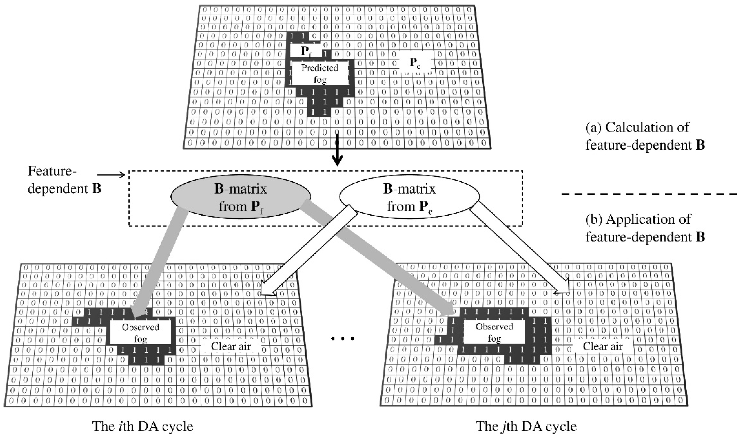
2.2. Design of Feature-Dependent B

The adopted GSI-based 3DVar system and its mathematical framework has been introduced by Wang [40]. In this system, B is a profound factor to produce the analysis increment through weighting the prior state, spreading the observation information, and applying a balance between the control variables (CVs) [41]. Because of the large dimensions, B cannot be explicitly calculated but can be modeled through several operators using

$$B=U_{\mathrm{p}}S{U}_{\mathrm{v}}{U}_{\mathrm{h}}{U}_{\mathrm{h}}^{\mathrm{T}}{U}_{\mathrm{v}}^{\mathrm{T}}{S}^{\mathrm{T}}{U}_{\mathrm{p}}^{\mathrm{T}}$$

(1)

Each operator was separately modeled to account for each elemental transform [42,43]. The set of CVs associated with the static B-matrix and their cross-variable correlations are denoted in the physical transform U_p. The matrices U_h and U_v are the spatial transforms, respectively, defining the horizontal and vertical autocorrelations of the CVs. The diagonal matrix S represents the standard deviations of the background errors of the CVs. Descombes et al. [43] provides more details on these operators and their specific calculations.

Since the atmosphere truth is not explicitly known, the estimation of background errors cannot be straightforward. In practice, forecast differences are used as the surrogate of background errors, because they are empirically assumed to have similar structures [44]. In the NMC method, the differences are calculated between forecasts valid at the same time with different initialization times. An alternative technique to calculate the static error statistics is the ensemble-based method (ENS) [45], where the forecast differences are the differences between two ensemble members, i.e., member i and member i + 1, where i denotes the sequence index of an ensemble member. Compared to the NMC method, the static error statistics from the ENS method have been demonstrated to improve the forecast quality [44,46]. Therefore, the ENS method was adopted to calculate the B-matrix in this study.

Figure 4. Schematic diagrams of the (a) calculation and (b) application of the feature-dependent B-matrix. In (a), a bidimensional geographical mask defined by the background ensemble is required to calculate the feature-dependent B-matrix, including B-matrices from P_f and P_c, which correspond to the foggy areas and clear air in the background, respectively. Based on this mask, P_f represents the sea fog bin consisting of the points labeled as 1, and P_c indicates the clear-air bin consisting of the points labeled as 0. During the DA update in (b), the same feature-dependent B-matrix is applied in all DA cycles. In each cycle, the other geographical mask provided by the observed sea fog distributions is used to apply error statistics from different bins at appropriate locations. See texts for the details.

Figure 4. Schematic diagrams of the (a) calculation and (b) application of the feature-dependent B-matrix. In (a), a bidimensional geographical mask defined by the background ensemble is required to calculate the feature-dependent B-matrix, including B-matrices from P_f and P_c, which correspond to the foggy areas and clear air in the background, respectively. Based on this mask, P_f represents the sea fog bin consisting of the points labeled as 1, and P_c indicates the clear-air bin consisting of the points labeled as 0. During the DA update in (b), the same feature-dependent B-matrix is applied in all DA cycles. In each cycle, the other geographical mask provided by the observed sea fog distributions is used to apply error statistics from different bins at appropriate locations. See texts for the details.

To increase the heterogeneity of B, the error statistics in Equation (1) were computed over domains with specified features, i.e., foggy area and clear air, separately. Like the operations for precipitation [22,25] and fog [21], a feature-dependent binning method is employed. The bins of a domain for foggy area and clear air were obtained through the bidimensional geographical mask, which is marked as 1 where the sea fog occurs at the surface level of a background ensemble member, otherwise, marked as 0 (Figure 4a). Specifically, the sea fog bin P_f (clear air bin P_c) represents the points where the surface liquid water content (LWC) is greater (smaller) than 0.016 g kg⁻¹ (the threshold for sea fog diagnostics from Zhou and Du [47] and W14) in two adjacent background ensemble members for the ENS method. Locations where two background members do not fall in the same threshold were omitted from the calculation of B-matrix, as this situation only occurs in the boundary of fog areas with small sample sizes. The grid points in P_f (P_c) comprise ~7.5% (~91.2%) of the computational domain in this study. Then each operator in Equation (1) is obtained by spatially averaging the error statistics over each bin. As in Michell et al. [22], the decomposed B of Equation (1) was modified to Equation (2):

$$\begin{array}{ll}B& =P_{\mathrm{f}}{U}_{\mathrm{p}}S{U}_{\mathrm{v}}{U}_{\mathrm{h}}{U}_{\mathrm{h}}^{\mathrm{T}}{U}_{\mathrm{v}}^{\mathrm{T}}{S}^{\mathrm{T}}{U}_{\mathrm{p}}^{\mathrm{T}}{P}_{\mathrm{f}}^{\mathrm{T}}\\ & +P_{\mathrm{c}}{U}_{\mathrm{p}}S{U}_{\mathrm{v}}{U}_{\mathrm{h}}{U}_{\mathrm{h}}^{\mathrm{T}}{U}_{\mathrm{v}}^{\mathrm{T}}{S}^{\mathrm{T}}{U}_{\mathrm{p}}^{\mathrm{T}}{P}_{\mathrm{c}}^{\mathrm{T}}\end{array}$$

(2)

As a result, the B-matrix computed from P_f and P_c were obtained (Figure 4a). As such, B-matrix can specify the feature of sea fog; we call them feature-dependent B.

During the 3DVar update, this study applied different error statistics from different bins simultaneously at appropriate locations guided by the geographical mask defined by the spatial distributions of the observed fog (Figure 4b). Such a relatively reliable geographical mask is expected by Ménétrier and Montmerle [21] for applying the feature-dependent B. To achieve this capability, we further extended GSI before the variational minimization by interpolating the feature-dependent B matrices into each analysis grid for foggy areas and clear air indicated by the geographical mask based on the observed fog. As shown in Figure 4b, the B-matrix from P_c was applied to the locations where is the clear air (labeled as 0), and the B-matrix from P_f was used within the observed fog (labeled as 1) in each DA cycle. Note that a discontinuity issue of the covariance function exists at the geographical mask border between the foggy areas and clear air, as discussed in Ménétrier and Montmerle [21]. To account for this issue, the same normalized Gaussian kernel with a length scale of 30 km proposed by Ménétrier and Montmerle [21] was applied to blur the mask border for smoothing the covariance functions (S, U_h, and U_v) from P_c and P_f. For brevity, the feature-dependent B is hereafter called Fog-B. In contrast, the homogeneous B computed over the entire domain comprising both foggy areas and clear air in W14 is hereafter referred to as Full-B. The 3DVar scheme using Fog-B keeps the same size of CVs with the use of Full-B by directly changing the static error statistics in foggy areas during the minimization. Therefore, a few extra computational costs are required.

2.3. Calculation of B-Matrix

Following the ENS method described above, the calculation of B-matrix needs an ensemble of forecast differences, obtained from the differences between two adjacent ensemble members. The datasets of an ensemble forecast were generated as follows. Firstly, a total of 125-member initial ensemble was produced by adding the “random_CV” perturbations to the corresponding European Centre for Medium-Range Weather Forecasts (ECMWF) Reanalysis v5 (ERA5) data. After, a 12 h WRF forecast was initialized from the initial ensemble, the required ensemble forecast was obtained. Specifically, the 12-h forecast of a total of 125-member ensemble is generated from the initial ensembles of five sea fog cases, valid at 1200 UTC 28 April 2007, 0000 UTC 9 April 2009, 0000 UTC 27 March 2012, 0000 UTC 20 May 2014, and 0000 UTC 28 March 2015. For each case, there is a 25-member ensemble forecast where most members can well capture a mature sea fog. The utility GEN_BE_v2.0 described in Descombes et al. [43] is then extended to compute each operator in Equation (2) to obtain the B-matrix. Note that we followed the option of “CV5” in WRFDA to develop the B-matrix. Therefore, no multivariate correlation between moisture CV and the other CVs is considered here, as in W14. The construction of B-matrix is also examined individually using the 12 h ensemble forecasts valid at 0000 UTC 10 April 2009, at 1200 UTC 28 March 2015, and at 0000 UTC 29 March 2015. Similar error statistics as shown in Section 4 were obtained. Therefore, the static error statistics for fog areas show fewer diurnal variations and is acceptable for analyzing the states of the fog regions in the 3DVar.

3. Numerical Experiments

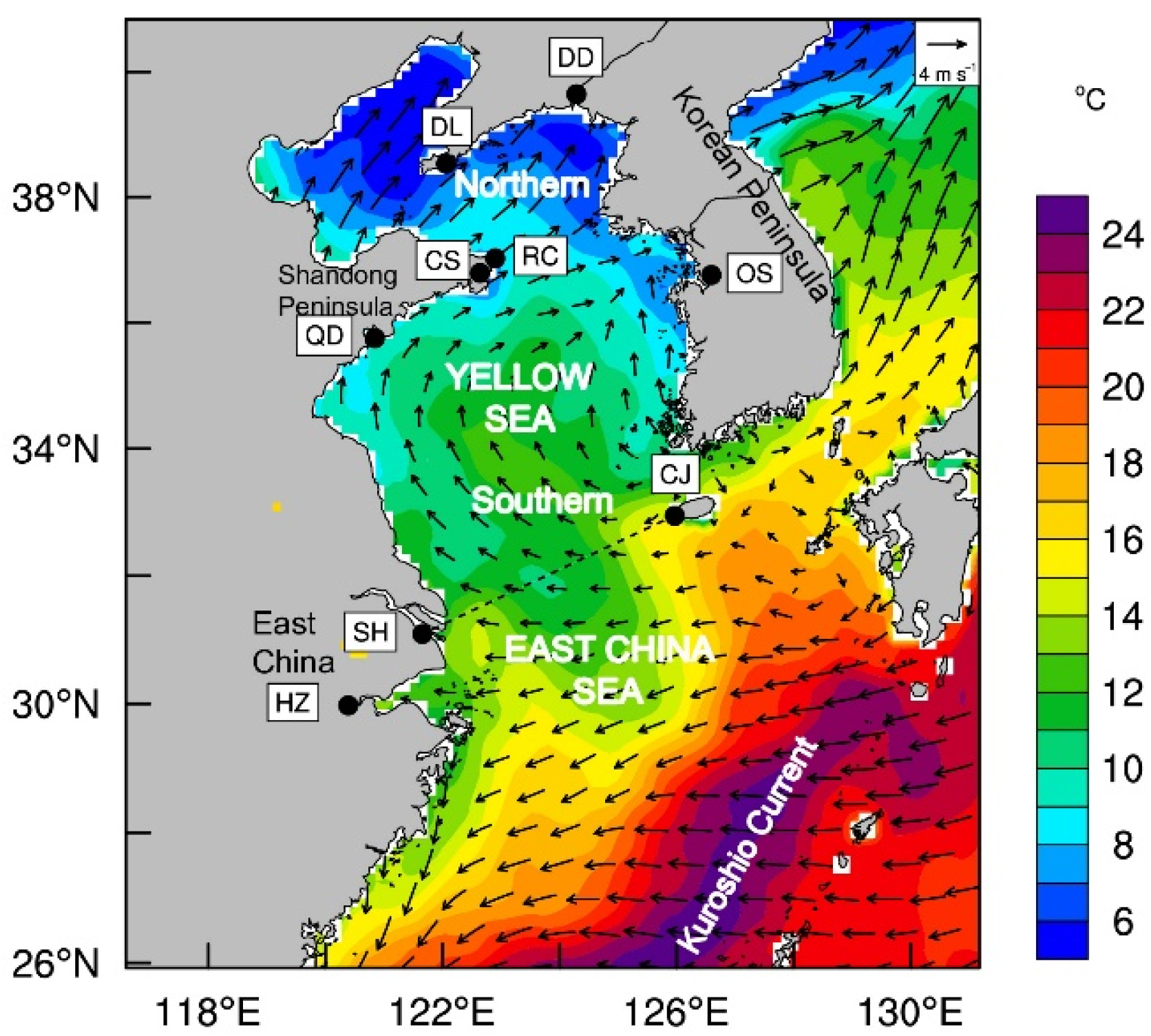
3.1. Case Overview

All three cases (Case07, Case09, and Case15) featured a similar synoptic system of a high-pressure system over the sea, which benefits the sea fog formation over the Yellow Sea [1,18,48]. Taking Case09 as an example, as shown in Figure 1, the warm moist air masses gathered over the Kuroshio Current region and the SST gradually decreased from south to north at 1200 UTC 9 April 2009. The southeasterly and easterly flows occurred in the south of a high-pressure system over the Yellow Sea. These flows led to the formation of the advection fog through transporting the warm moist air westward over the cold sea surface. Hourly evolution of the satellite-derived sea fog (namely, the observed fog) shows that the sea fog patches initially formed over the border between the southern Yellow Sea and the East China Sea. The sea surface with a sharp SST gradient promoted the cooling and condensation of the advected warm moist air [1,2,18,49]. The sea fog patches gradually extended and enlarged when the warm moist air was continually advected over the cold sea surface.

In addition, Case07 is characterized by a short-lived sea fog with a small areal coverage along the southern coast of Shandong Peninsula, persisting from 1900 UTC 28 April to 0600 UTC 29 April 2007. Case15 is a long-lived sea fog that occupied nearly a half portion of the Yellow Sea from 1800 UTC 28 March to 0000 UTC 29 March 2015. Case07 was first chosen to understand the impact of Fog-B on the analyses and forecasts in Section 4. In Section 5, all three cases were used to evaluate the performance of Fog-B for the forecasts of sea fog and MABL moisture conditions.

3.2. Model Configuration

The Advanced Research WRF (Version 3.9.1) was employed in this study. A single domain centered at (34.2°N, 124.1°E) uses a 15 km grid spacing with 240 × 240 horizontal grid points (Figure 2). With the model top up to 100 hPa, 50 full-η levels (η_n ranges between 1.0 and 0.0) are assigned in vertical. Consistent with previous numerical predictions of sea fog over the Yellow Sea, 16 full-η levels are placed within the lowest 1 km [11], and the lowest model level (between η₁ = 1.0 and η₂) height is specifically set to ~8 m [14] for better capturing the MABL processes and their interactions near the sea surface.

The model physics configuration includes the Yonsei University (YSU) planetary boundary layer scheme [50,51], the corresponding fifth-generation Mesoscale Model (MM5) Monin-Obukhov surface layer scheme [52,53], the Lin microphysics scheme [54], the Rapid Radiative Transfer Model for General circulation models (RRTMG) longwave and shortwave radiation schemes [55], the Kain–Fritsch cumulus scheme [56,57], and the unified Noah land surface model [58].

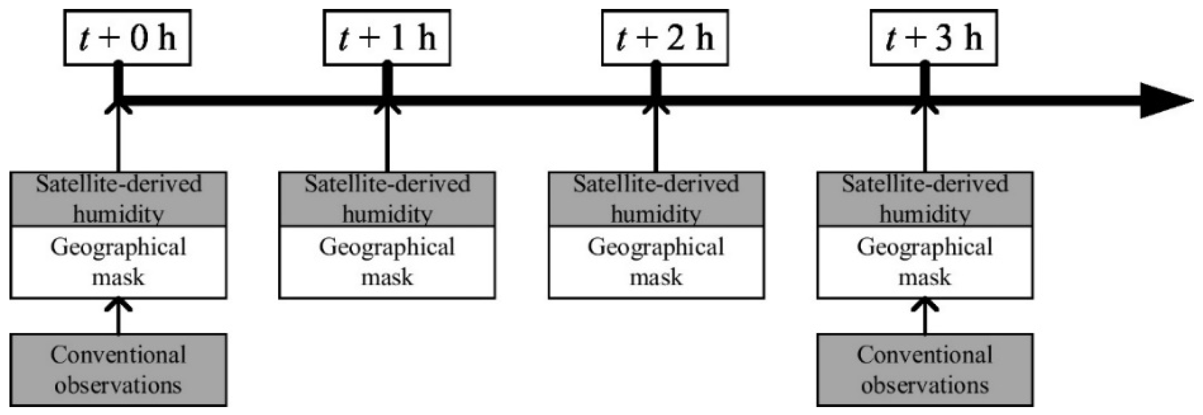
3.3. Assimilation and Forecast Experiments

The initial and lateral boundary conditions were interpolated from the ERA5 data (0.25 × 0.25°, 3 hourly). The cycling setup of the GSI-based 3DVar DA system is presented in Figure 5. Starting at t + 0 h, the conventional data (i.e., routine radiosonde and surface measurements) are assimilated every 3 h, and satellite-derived humidity data are hourly assimilated ahead to t + 3 h. The starting time t + 0 h for each case depends on the occurrence of sea fog. At each satellite-derived humidity assimilation cycle, the observation-based geographical mask was applied to guide the application of Fog-B (Figure 4b). A 6-h free forecast is initialized every hour from t + 0 h to t + 3 h. Specifically, the 3 hourly conventional DA and hourly satellite-derived humidity DA were conducted from 1800 UTC to 2100 UTC 9 April 2009 for Case09, and from 1800 UTC to 2100 UTC 28 March 2015 for Case15. For Case07, as the sea fog initiated at 1900 UTC 28 April 2009, the conventional data were assimilated from 1800 UTC to 2100 UTC, but the satellite-derived humidity is assimilated from 1900 UTC to 2100 UTC. Therefore, each experiment has a total of 11 forecasts with a 6 h leading time initialized from the analyses with the satellite-derived humidity assimilation for the three cases. Hourly archived model outputs were used for the evaluations in Section 5.

In this study, three experiments (noMT, Q_full and Q_fog) were designed for each targeted case, i.e., Case07, Case09, and Case15 (

Table 1. List of experiments.

Experiment	If Assimilating Satellite-Derived Humidity	B Type for Satellite-Derived Humidity Assimilation
noMT	No	—
Q_full	Yes	Full-B
Q_fog	Yes	Fog-B

). Specifically, noMT only assimilates the conventional observations, while both satellite-derived humidity and conventional observations are assimilated in the remaining two experiments. Using q as the moisture CV [21], Q_full uses Full-B to assimilate satellite-derived humidity, while Q_fog uses Fog-B. Full-B is also used in the conventional DA for all experiments. The B-matrix calculated from the 125-member ensemble in Section 2.3 was employed for all three targeted cases. Studies of single-observation tests and the first DA cycle were separately conducted for Case07 to understand the impact of feature-dependent B on the analyses and forecasts. Subsequently, continuously cycled DA were conducted for the three targeted cases. Comparisons between noMT and the satellite-derived humidity assimilation experiments were used to examine the effectiveness of assimilating satellite-derived humidity for the sea fog forecasts. The comparison between Q_full and Q_fog is performed to investigate the effects of feature-dependent B on the forecasts of sea fog coverage and MABL moisture conditions.

4. Understanding the Impact of Feature-Dependent B on the Analyses and Forecasts

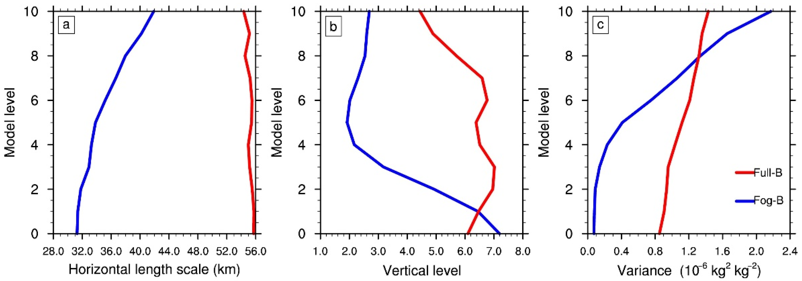
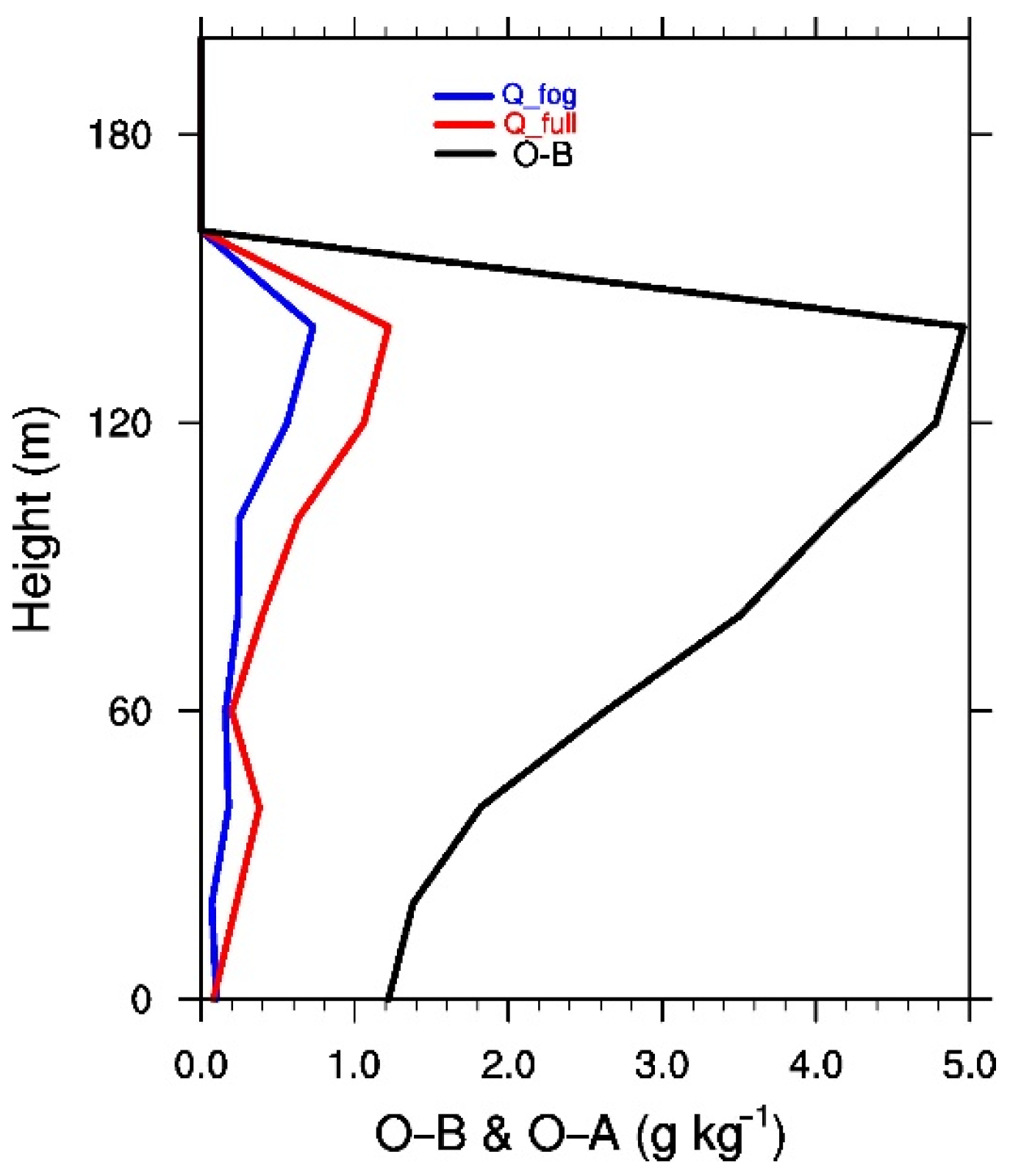
4.1. Difference in Error Statistics between Fog-B and Full-B

We first present the different behaviors between Fog-B and Full-B in the error statistics. Figure 6 shows the error statistics below the 10th model level (~400 m), which primarily reflects the error characteristics for the low-level MABL. The horizontal length scale varies a little at each level for Full-B, and so is for Fog-B below the 5th model level, but it gradually increases along with the height above that (Figure 6a). In general, the horizontal length scale in Full-B is 12–24 km larger than that in Fog-B below the 10th level. Like Michel et al. for clouds [22], Fog-B has smaller horizontal length scales probably because a significant part of the background error here is associated with microphysical processes. The vertical length scale represents the height of vertical mixing. Fog-B has a similar, but slightly larger vertical length scale than Full-B near the surface, and the vertical length scale in Full-B is consistently much broader than that in Fog-B above the 2nd model level (Figure 6b). These results may reflect the thermal inversion layer around the fog top constrains the vertical extension in the upper level of the fog layer, and the intensive mixing near the surface within fog. In terms of the background error variance, Fog-B has consistently smaller values than Full-B below the 8th model level (~300 m), especially under the 4th model level (~60 m; Figure 6c). The smaller variances in Fog-B reflect the well-mixing within sea fog [12,18]. This result is opposite to the findings of Michel et al. [22] showing that larger errors exist in convective clouds than clear air. This can be explained by the fact that convective clouds have strong changes in dynamic and thermodynamic fields, in contrast, fog with well-mixed cloud liquid water usually occurs within stable MABL stratification conditions with fewer state changes. In a word, Full-B generally has broader horizontal and vertical length scales and larger error variances than Fog-B below ~300 m height, except near the surface where Fog-B has a slightly larger vertical length scale than Full-B.

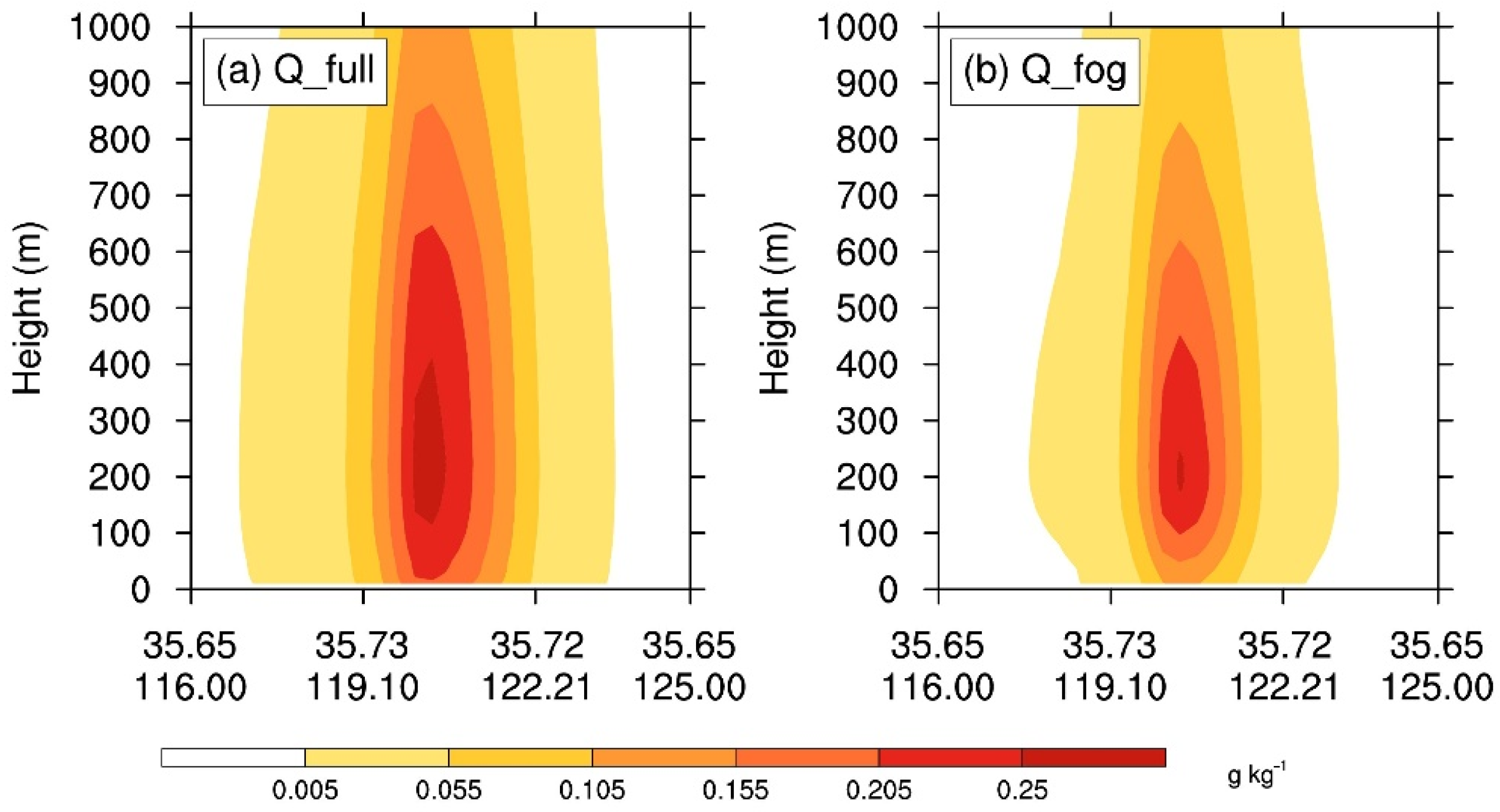
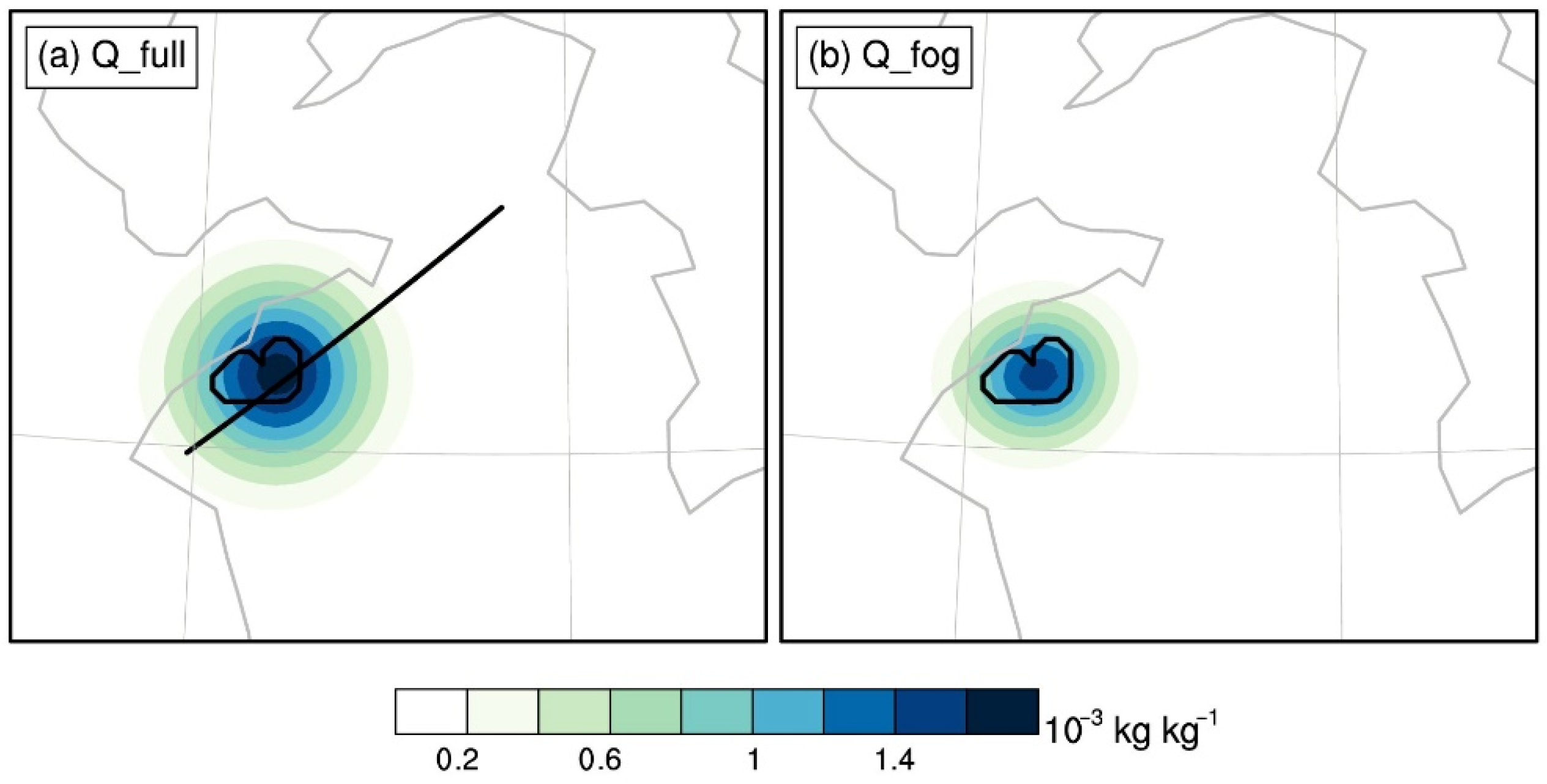
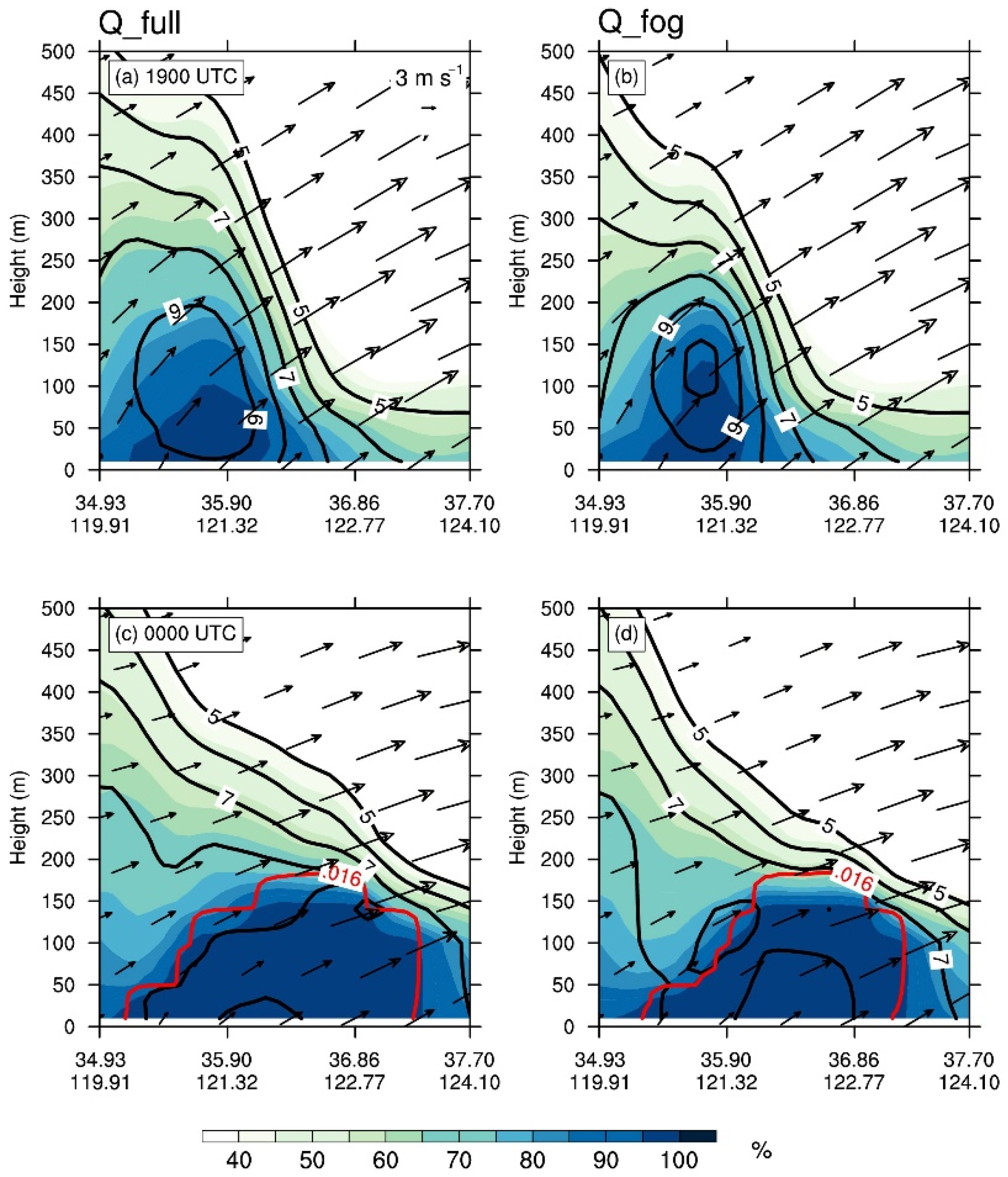
4.2. Differences in Analyses and Forecasts between Experiments Using Fog-B and Full-B

To preliminarily examine the impact of Fog-B on the analysis increments, Q_full and Q_fog with the assimilation of a single observation were performed for Case07. We assimilate an artificial q observation with an innovation of 0.5 g kg⁻¹ at 1000 hPa of the location (35.65°N, 120.54°E) in both experiments. The background field is provided by the ERA5 data valid at 1900 UTC 28 April 2007. Figure 7 shows the analysis increments of the water vapor mixing ratio (Qvapor) for the two experiments. Q_full produces much broader horizontal distributions of Qvapor increments than Q_fog. Moreover, the magnitude of Qvapor increments with the use of Fog-B is ~0.05 g kg⁻¹ smaller than that using Full-B. These apparent differences between Q_full and Q_fog in Qvapor increments are a straightforward consequence of the differences between Full-B and Fog-B in the horizontal length scale and error variance. Both experiments share a similar vertical extension of Qvapor increments probably because the vertical length scales of Fog-B and Full-B differ very little near the surface.

With the assimilation of full satellite-derived humidity data at 1900 UTC 28 April 2007, the analysis increments from Q_full and Q_fog were also compared for Case07 (Figure 8). Q_full yields larger and more widespread Qvapor increments than Q_fog, consistent with the single-observation experiments (Figure 7). Notably, the added Qvapor in Q_full extends severely outside of the observed fog areas (Figure 8a). In contrast, the coverage of Qvapor increments in Q_fog is more consistent with the observed fog areas (Figure 8b).

Subsequently, we further compared Q_full and Q_fog to show how their analyses fit to the observations (O–A) in Figure 9, where O stands for the observed q converted from the satellite-derived humidity, and A is the analyzed q. Both experiments share the same deviation (O–B) between the observed q and the background q, and such deviation is significantly reduced by up to 4.0 g kg⁻¹ through the satellite-derived humidity assimilation. The analysis produced by Q_fog fits closer to the observations than that by Q_full. Q_fog has 0.1–0.6 g kg⁻¹ smaller O–A than Q_full, especially below 80 m. However, the better fitting to observations at the analysis time does not necessarily mean an improved analysis [59]. The quality of the analysis should be evaluated by verifying the subsequent forecasts. Figure 10 presents the cross-sections of the analyses at 1900 UTC 28 April 2007 and 5-h forecasts valid at 0000 UTC 29 April 2007 from Q_full and Q_fog. Results indicate that the distributions of the near-saturation (indicated by RH ≥ 95%) agree well with the horizontal coverage of Qvapor increments at the analysis time (Figure 10a,b vs. Figure 8). Compared to Q_fog, the greater and more widespread Qvapor increments in Q_full lead to a more widespread saturated air near the surface. In the subsequent forecasts, the added moisture at 1900 UTC is transported northeastward and condenses into fog due to the cold sea surface along with the prevailing wind. The greater and more widespread Qvapor increments result in more widespread sea fog in the later forecasts. Therefore, Q_full produces more widespread sea fog than Q_fog facilitated by the southwesterly advection at 0000 UTC (Figure 10c,d).

To conclude, we found that (1) Full-B generally has broader horizontal and vertical length scales and larger error variances than Fog-B below ~300 m, except near the surface where the vertical length scale of Fog-B is slightly broader than that of Full-B; (2) using Full-B tends to add greater and more widespread Qvapor increments and thus predicts sea fog with a larger areal coverage than using Fog-B. These results indicate that the behavior of Qvapor increments is a straightforward consequence of the static error statistics and strongly affects the predicted sea fog distributions facilitated by the effects of moisture advection.

5. Evaluating the Role of Feature-Dependent B in Sea Fog Coverage Forecasts

In Section 4, we aim to understand how the feature-dependent B affects the analyses and the subsequent forecasts of sea fog coverage. In this section, the systematic evaluation of the impact of Fog-B on sea fog forecasts, including sea fog coverage and MABL moisture conditions, is performed through multiple-case studies. The overall skills of sea fog forecasting are evaluated over 11 forecasts from three cases for each experiment.

5.1. Sea Fog Coverage

According to Stoelinga and Warner [60], Vis is calculated as a function of the extinction coefficient that is related to hydrometeors, such as the mixing ratios of cloud liquid water, rain, cloud ice, and snow. Given that only the cloud liquid water is included in sea fog over the Yellow Sea, the extinction coefficient can be parameterized using the LWC at low levels as in Kunkel [61]. Hence, a threshold of 0.016 g kg⁻¹ for the LWC at the lowest model level that is equivalent to the 1 km Vis from the fog definition [7] is obtained. This threshold has been used to identify the bins of P_f and P_c in Section 2.2. In addition, Zhou and Du found that the fog-top height of the advection fog rarely exceeds 400 m [47]. Therefore, the criteria adopted to diagnose the predicted sea fog coverage are the view from the fog top that is defined when LWC ≥ 0.016 g kg⁻¹ using a top-down manner and the fog-top height ≤ 400 m, which are commonly used in the previous sea fog numerical studies [10,11,12,13,14,47,62].

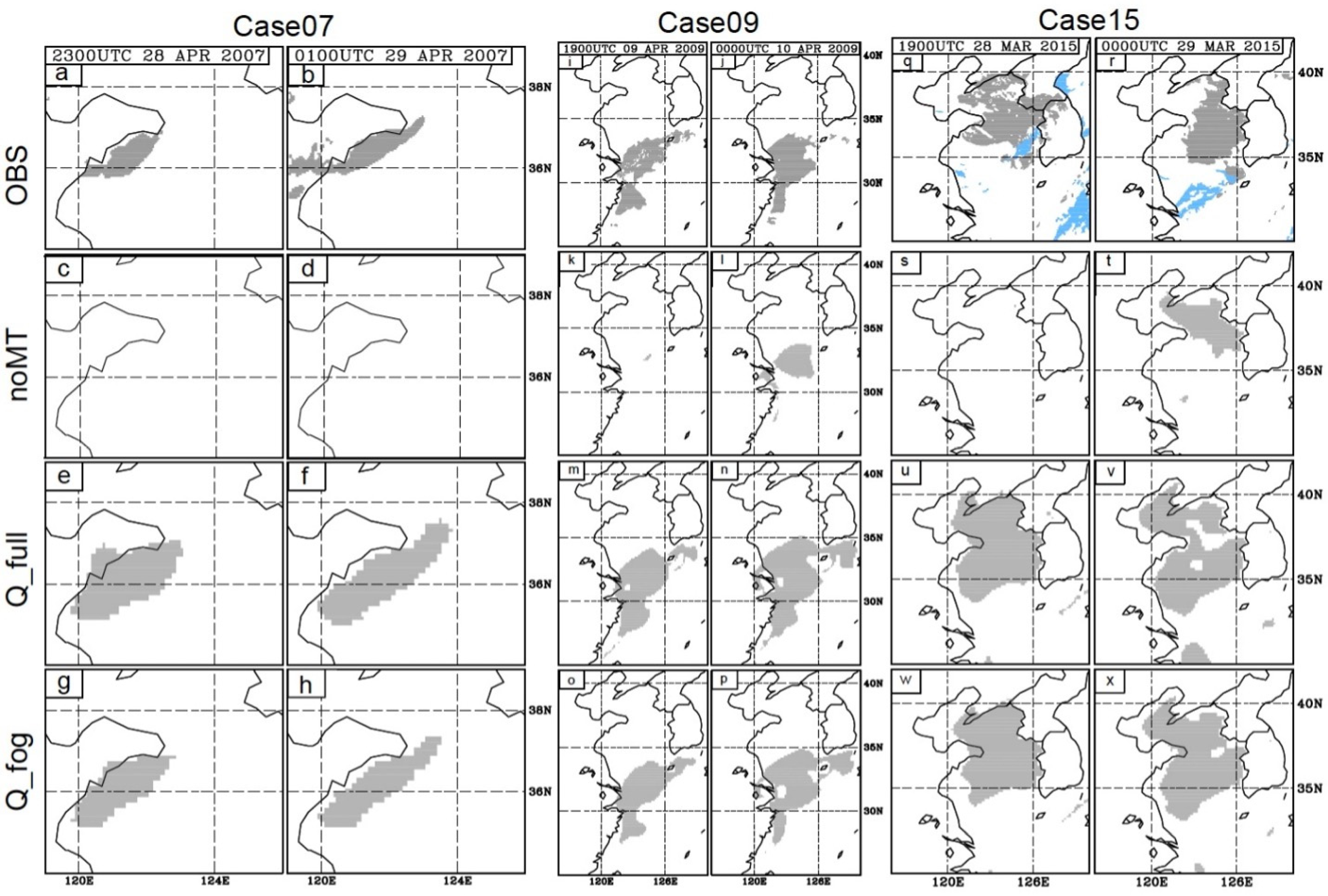
5.1.1. Subjective Evaluation

Through examining the spatial distributions of the predicted sea fog, we found that the impact of Fog-B keeps consistent among all forecasts for the three cases. In Figure 11, the sea fog forecasts of noMT, Q_full, and Q_fog initialized from the first satellite-derived humidity DA cycle for each case are shown and verified against the observed fog.

The 2- and 4-h forecasts initialized at 2100 UTC 28 April 2007 for Case07 are shown in Figure 11c–h. The effectiveness of assimilating satellite-derived humidity is first demonstrated since noMT completely misses the observed sea fog while Q_full and Q_fog can capture it. Consistent with the discussions in Section 4, Q_full tends to produce a more widespread sea fog than Q_fog. The sea fog distributions in Q_full are nearly two times larger than the observed sea fog coverage (Figure 11e,f vs. Figure 11a,b), and the overestimated sea fog spreads northeastward approaching 124°E. In contrast, Q_fog has a better performance than Q_full because of its smaller predicted sea fog coverage closer to the observations (Figure 11g,h vs. Figure 11a,b).

Figure 11k–p present the 1- and 6-h forecasts initialized at 1800 UTC 9 April 2009 for Case09. Like in Case07, noMT needs a longer time to spin up and significantly underestimates the observed fog, and the sea fog distributions in Q_full are larger than those in Q_fog. At 1900 UTC, two sea fog patches were observed over the southern Yellow Sea and the East China Sea (Figure 11i). The northern patch stretched across the south of the Yellow Sea and the southern patch was located in the northwest of the East China Sea. Q_fog well captures these patterns (Figure 11o), while the two patches have severely extended in Q_full (Figure 11m). Then the southern fog patch was observed stretching along the coastal at 0000 UTC 10 April (Figure 11j), which is better produced by Q_fog with smaller sea fog coverage than Q_full (Figure 11n,p). Therefore, Q_fog performs the best in the sea fog coverage forecasts among the three experiments.

For Case15, Figure 11s–x show the 1- and 6-h forecasts initialized at 1800 UTC 28 March 2015. It is found that both Q_fog and Q_full improve sea fog forecasting upon noMT. Consistent with Case07 and Case09, Q_fog predicts lesser widespread sea fog distribution than Q_full, especially for the southern sea fog area (Figure 11u–x). Therefore, while both Q_full and Q_fog overestimate the observed fog, the sea fog coverage in Q_fog is closer to the observation than in Q_full.

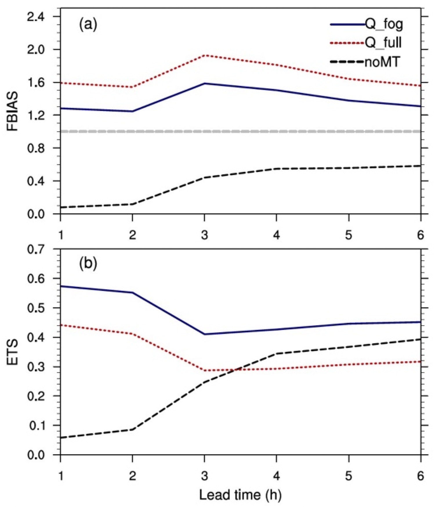
5.1.2. Quantitative Evaluation

Subsequently, the statistical scores of frequency bias (FBIAS) and equitable threat score (ETS) are employed to quantitatively evaluate the predicted sea fog distributions. These scores are introduced and widely used in many studies on sea fog [10,12,13,14,15,47]. The FBIAS score is defined as $\mathrm{FBIAS}=\frac{F}{O}$, where F and O represent the number of points for forecasted and observed fog areas, respectively. Therefore, it represents the relative size of the forecast and observed fog distributions, i.e., a larger FBIAS score means a larger forecast sea fog coverage, and the FBIAS score close to 1.0 means that the size of the forecast sea fog area is comparable to the observed one. The ETS with the perfect score of 1.0 is considered as a comprehensive verification score [63]. Using H denotes the number of correctly forecast points, $\mathrm{ETS}=\frac{H-R}{F+O-H-R}$, where $R=\frac{F\times O}{N}$ is a random hit penalty, and N refers to the grid size of the verification domain. Figure 12 presents the time series of the scores of FBIAS and ETS aggregated over the 11 1–6 h forecasts from three cases for each experiment. The forecast skills evaluated by these statistics are consistent with the subjective evaluations in Section 5.1.1.

Among all experiments in Figure 12a, Q_full has the highest FBIAS scores exceeding 1.5 for all lead times, which indicates the significant overestimation of sea fog distribution. The FBIAS scores of Q_fog are greater than 1.0 but closer to 1.0 than those of Q_full, suggesting that Q_fog has relatively comparable sea fog coverage with the observations. Experiment noMT severely underestimates the observed fog coverage with the lowest FBIAS scores smaller than 0.6 for all lead times, especially at the first two lead times. As a larger FBIAS score means a larger forecast sea fog coverage, the FBIAS scores in Figure 12a also reflect the relative size of the areal coverage of the predicted sea fog over the 11 forecasts from the three cases for each of the three designed experiments. In general, Q_full has the largest predicted sea fog coverage, followed by Q_fog, and noMT has the smallest. These results are consistent with the forecasts initialized from the first satellite-derived humidity DA cycle in Figure 11.

In terms of the ETSs (Figure 12b), Q_fog has the highest forecast skills with its ETSs larger than 0.4 throughout the entire forecast period. The ETSs in Q_full are ~0.1 smaller than those in Q_fog because of its consistent overestimation of sea fog coverage. The ETSs due to the satellite-derived humidity decrease after the 2nd lead time and start to level off after the 3rd lead time. The decreased ETSs are consistent with the increased FBIASs, indicating the overestimated sea fog coverage in this period. Such reduced ETSs may be related to the overestimated moisture at the analysis time as the temperature is not changed in the assimilation. This overestimated moisture is carried over in the subsequent forecasts. It is suggested that additional efforts are required to further advance methods for assimilating the satellite-derived humidity, including to further refine B. While noMT fails to spin up in the earlier forecast stage, its sea fog coverage gets broader since the forecast lead time of 3 (Figure 12a). As a result, noMT has the lowest forecast skills at 1–3 lead times, and its ETSs become larger after the 3rd lead time, leading to around 0.05 higher compared to Q_full.

The aggregated statistical scores temporally averaged over the 1–6 h lead times are listed in

Table 2. Aggregated statistical scores averaged over the 1–6-h forecasts initialized every hour during the DA period from three cases for designed experiments. The marker # indicates the statistical significance at the confidence level of 95%.

Experiment	FBIAS	ETS	ETS Improvements (%)
			Q_Full	Q_Fog
noMT	0.387	0.249	37.80%	91.6% #
Q_full	1.678	0.343	—	39.1% #
Q_fog	1.383	0.477	—	—

. This result obeys the above subjective and objective evaluations for the predicted sea fog distributions. It shows that noMT predicts the smallest sea fog area with the lowest FBIAS score (0.387) and has the worst performance with the lowest ETS of 0.249. In contrast, Q_fog has the highest forecast skill with the ETS of 0.477, which is 0.134 greater than that of Q_full. The inferior skill of Q_full mostly results from its significantly overpredicted sea fog indicated by the largest FBIAS score of 1.678. Furthermore, the ETS improvements are calculated between any two experiments (relative to experiments in the first column of Table 2). Compared to noMT, Q_fog significantly improves the sea fog coverage forecasts with the ETS improvement higher than 91%, and Q_full has only 37.8% improvement. Between the experiments with the satellite-derived humidity assimilation, Q_fog performs significantly better than Q_full with an improvement of 39.1%. A Student’s t-test was applied to the ETS improvements to test whether the improvement between any two experiments is statistically significant. Results show that the improvements of Q_fog relative to noMT and Q_full well pass the significant test with a confidence interval of 95%.

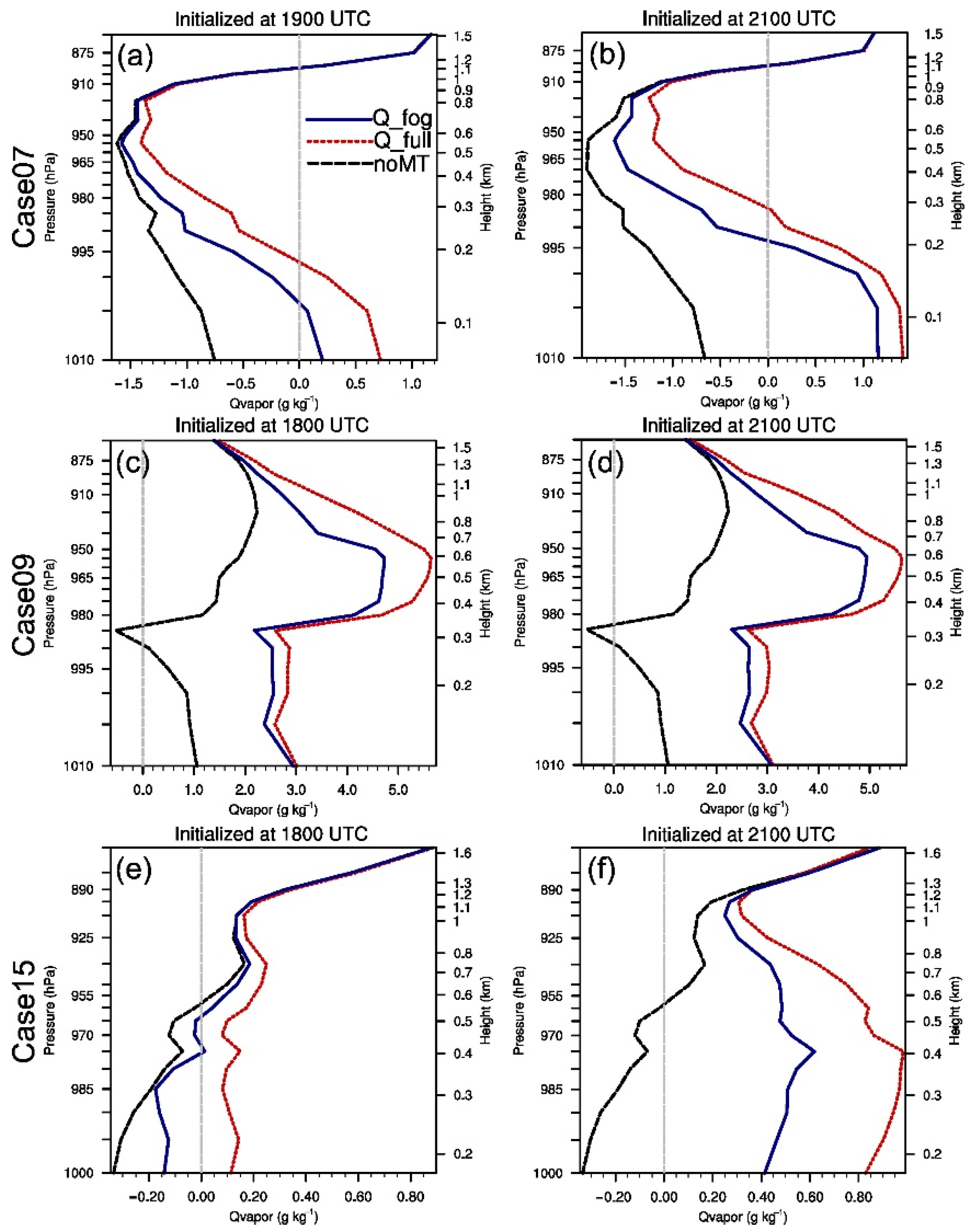
5.2. MABL Moisture Conditions

Previous studies have shown that the distribution of advection fog highly relies on the saturation conditions near the sea surface [10,12,14,18,64]. From the physical perspective, sea fog formation and maintenance are strongly affected by the temperature and moisture conditions within the MABL. The satellite-derived humidity assimilation aims to improve the MABL moisture conditions favorable for sea fog evolutions. Given the lack of routine observations over the ocean, the soundings (black dots in Figure 1) along the coast in the onshore wind near the sea fog are selected to represent the marine environment associated with the sea fog. In this study, the Qvapor measurements of the selected soundings are chosen to assess the MABL moisture conditions, especially near the surface associated with the sea fog evolution during the forecast period. The agreement between the model and observations over the selected soundings were evaluated using the bias, which is defined by averaging the difference between the forecasted and observed Qvapor with the best value of 0.0 g kg⁻¹. For each case, the forecasts from all DA cycles have a similar pattern of Qvapor biases for each experiment. Some forecasts compared against the soundings are selected and shown in Figure 13.

For Case07, the forecasts valid at 0000 UTC 29 April 2007 initialized at 1900 UTC and 2100 UTC 28 April were verified against the soundings at QD and CS (Figure 13a,b). Experiment noMT experiences drying biases below 1.1 km, which are about –0.75 g kg⁻¹ near the surface and up to –1.6 g kg⁻¹ around 500 m (Figure 13a). With the satellite-derived humidity assimilation at 1900 UTC, the forecasted Qvapor profiles from Q_full and Q_fog are adjusted toward the observations following the characteristics of their own applied B-matrix. Relative to noMT, both Q_full and Q_fog alleviate the drying biases below 1.0 km. Q_full has 0.25–0.5 g kg⁻¹ greater amounts of Qvapor than Q_fog, which reflects the greater error variance in Full-B (Figure 6). Below 150 m, Q_full has up to 0.7 g kg⁻¹ wetting biases, and it has the maximum drying biases of ~1.25 g kg⁻¹ above 300 m. The wetting biases in Q_fog is ~0.2 g kg⁻¹ and ~0.5 g kg⁻¹ smaller than Q_full below 150 m, while Q_fog has the drying biases up to 1.5 g kg⁻¹ above 150 m. Similar results are also seen from the forecasts initialized at 2100 UTC (Figure 13b). Both Q_fog and Q_full alleviate the drying biases in noMT. While both Q_fog and Q_full have increased wetting biases, Q_fog still has ~0.25 g kg⁻¹ smaller wetting biases than Q_full below 200 m. Therefore, the MABL moisture conditions at low levels are better forecasted by Q_fog than by Q_full.

The forecasts valid at 0000 UTC 10 April 2009 initialized from the analyses at 1800 and 2100 UTC 9 April were verified against the soundings at Shanghai, Hangzhou, and Chejudo (CJ) (Figure 13c,d). Figure 13c shows positive Qvapor biases below 1.5 km in noMT except negative Qvapor biases around 300 m, which indicates that the predicted MABL in noMT is up to 2.2 g kg⁻¹ wetter than the observations. The satellite-derived humidity assimilation at 1800 UTC significantly changes the Qvapor profile of the 6 h forecast through humidifying the air. The wetting biases of Q_full generally are 0.1–1.0 g kg⁻¹ larger than those of Q_fog. These results are consistent with the differences between Full-B and Fog-B in the error variance (Figure 6). Similar differences in the Qvapor biases among the three experiments can also be found in the 3 h forecasts initialized at 2100 UTC (Figure 13d). Given that noMT already presents wetting biases throughout the whole levels except the height around 300 m, there is no need to further add moisture within the MABL for this case. Therefore, the magnitudes of Qvapor positive biases in Q_full and Q_fog are similar to those in Figure 13c. As this case has wetting biases in noMT, it is unreasonable to further increase moisture through the satellite-derived humidity assimilation. Simultaneously adjusting temperature and moisture may be required. Yang et al. [15] alleviated this issue by proposing an alternative observation operator to assimilate the satellite-derived humidity.

The forecasts valid at 0000 UTC 29 March 2015 initialized from the analyses at 1800 and 2100 UTC 28 March were evaluated using the soundings at Rongcheng, Dalian, Dandong, Oscan, QD, and CJ (Figure 13e,f). We notice drying biases up to ~0.35 g kg⁻¹ in noMT below ~550 m for the 6 h forecasts initialized at 1800 UTC (Figure 13e). Similar to Case07 and Case09, the satellite-derived humidity assimilation further increases Qvapor upon noMT, and the forecasted Qvapor changes following the characteristics of the applied B-matrix in each experiment. Specifically, Q_full has ~0.15 g kg⁻¹ wetting biases below 1.2 km on average. Q_fog still has drying biases below 500 m, which get significantly smaller than those of noMT, especially below 300 m, and its wetting biases above 500 m is 0.05–0.1 g kg⁻¹ smaller than Q_full. For the 3 h forecast initialized at 2100 UTC (Figure 13f), noMT still has negative biases below ~550 m. This result further demonstrates that the cycling assimilation of conventional observations is unable to sufficiently correct the drying biases in the MABL. The positive biases in Q_full get much larger and the negative biases in Q_fog turn into positive due to the cycling assimilation of satellite-derived humidity. Q_fog with smaller Qvapor biases is closer to the observations than Q_full as a result of their used static error statistics.

We also evaluated the wind and temperature forecasts in the MABL by comparing the temperature and wind measurements of the selected soundings with the corresponding forecasts (not shown). Small differences (below 1.0 m s⁻¹) in the wind fields among the three experiments are shown for the three cases. For the temperature field, all experiments have warm biases at low levels. Q_fog and Q_full reduce the warm biases compared to noMT. It was found that the performance of the temperature forecasts for Q_full and Q_fog depends on the stage of sea fog evolution. For example, Q_fog has smaller warm biases in the dissipated fog stage and larger warm biases in the mature fog stage than Q_full. As the temperature is not adjusted in the assimilation of the satellite-derived humidity due to the design of B in this study, the differences in temperature among the three experiments largely result from their different sea fog forecasts, which are mostly affected by the Qvapor analyses.

Overall, using noMT as the baseline, Q_full has larger Qvapor increases in the forecasts than Q_fog. It was found that the amounts of these Qvapor increases for the forecasts of Q_fog and Q_full are consistent with their corresponding Qvapor increments in Section 4. In other words, the differences in the analyses between Q_fog and Q_full were carried over in the subsequent forecasts. The Qvapor forecasts directly affected by the analyzed Qvapor in these results are similar to the diagnostics of single-cycle tests in Figure 10. Therefore, the overall skills of sea fog forecasts (Figure 12 and Table 2) agree well with the magnitudes of the Qvapor biases in the low levels during the forecasting (Figure 13) as well as the Qvapor increments at the analysis time in Q_full and Q_fog (Figure 7 and Figure 8). Compared to Q_full, the higher forecast skills obtained by Q_fog correspond well with its more properly analyzed Qvapor increments.

6. Conclusions and Discussion

Assimilating satellite-derived sea fog information (satellite-derived humidity) using the 3DVar was proposed by W14. Although this method produced encouraging results in improving the sea fog forecasts and associated moisture conditions of the marine atmospheric boundary layer (MABL), the sea fog coverage for many cases was overpredicted in W14 using a homogeneous static background error covariances (B) computed over the entire computational domain (Full-B). This study aims to further improve the sea fog coverage forecasts by developing a feature-dependent, heterogeneous B (Fog-B) within the GSI-based 3DVar system when the satellite-derived humidity is assimilated. In Fog-B, the static error statistics for sea fog areas and clear air are calculated separately using a feature-dependent binning method. The resultant Fog-B was applied simultaneously at appropriate locations guided by the observed sea fog derived from the satellite products.

It was found that Full-B generally has broader horizontal and vertical length scales and larger error variances than Fog-B below ~300 m except for the vertical length scale near the surface. Diagnostics and comparisons were performed to understand and examine the impact of Fog-B on analyses and forecasts of the sea fog, including sea fog coverage and MABL moisture conditions. Results show that the distribution and magnitude of the water vapor mixing ratio (Qvapor) analysis increments are a straightforward consequence of the static error statistics and then affect the sea fog forecasts. The Qvapor increments analyzed using Fog-B are narrower with a smaller magnitude than those using Full-B, leading to smaller sea fog coverage in the subsequent forecasts. Verifications against the observations show that using Fog-B performs better than using Full-B in the forecasts of sea fog coverage and the MABL moisture conditions for three sea fog cases over the Yellow Sea.

As an initial effort of optimizing the satellite-derived humidity assimilation, this study aimed to illustrate the necessity of applying the feature-dependent B to foggy areas for improving the forecasts of sea fog coverage. The predicted sea fog in this study mostly occurred between midnight and late morning. Systematic experiments using more cases across a full day will be warranted for more robust conclusions. Figure 13 shows that Fog-B alleviates the positive Qvapor biases in Full-B but still overestimates the Qvapor. Further efforts are required to refine the feature-dependent B, such as the selection of control variables [59], the inclusion of cross-variable correlations between moisture and temperature [16], etc. Moreover, the assimilation of satellite-based clear air observations [37,65] with the feature-dependent B for suppressing spurious fog and the systematic observation error validation need further investigation.

References

1. Wang, B. Sea Fog; China Ocean Press: Beijing, China, 1985. [Google Scholar]
2. Koračin, D.; Dorman, C.E. Marine fog: Challenges and Advancements in Observations, Modeling, and Forecasting; Springer International Publishing: San Diego, CA, USA, 2017. [Google Scholar]
3. Lewis, J.M.; Koračin, D.; Redmond, K.T. Sea fog research in the United Kingdom and United States. Bull. Am. Meteorol. Soc. 2004, 85, 395–408. [Google Scholar] [CrossRef]
4. Zhang, S.; Bao, X. The main advances in sea fog research in China. J. Ocean Univ. China 2008, 38, 359–366. [Google Scholar] [CrossRef]
5. Zhang, S.; Xie, S.; Liu, Q.; Yang, Y.; Wang, X.; Ren, Z. Seasonal variations of Yellow Sea fog: Observations and mechanisms. J. Clim. 2009, 22, 6758–6772. [Google Scholar] [CrossRef]
6. Fu, G.; Zhang, S.; Gao, S.; Li, P. Understanding of Sea Fog over the China Seas; China Meteorological Press: Beijing, China, 2012. [Google Scholar]
7. WMO. International Meteorological Vocabulary; World Meteorological Organization: Geneva, Switzerland, 1966. [Google Scholar]
8. Gao, S.; Wang, Y.; Fu, G. Ensemble forecast of a sea fog over the Yellow Sea. J. Ocean Univ. China 2014, 44, 1–11. [Google Scholar] [CrossRef]
9. Lu, X.; Gao, S.; Rao, L.; Wang, Y. Sensitivity study of WRF parametrization schemes for the spring sea fog in the Yellow Sea. J. Appl. Meteorol. Sci. 2014, 25, 312–320. [Google Scholar]
10. Wang, Y.; Gao, S.; Fu, G.; Sun, J.; Zhang, S. Assimilating MTSAT-derived humidity in nowcasting sea fog over the Yellow Sea. Wea. Forecast. 2014, 29, 205–225. [Google Scholar] [CrossRef]
11. Yang, Y.; Gao, S. Sensitivity study of vertical resolution in WRF numerical simulation for sea fog over the Yellow Sea. Acta Meteorol. Sin. 2016, 74, 974–988. [Google Scholar] [CrossRef]
12. Yang, Y.; Gao, S. The impact of turbulent diffusion driven by fog-top cooling on sea fog development. J. Geophys. Res. Atmos. 2020, 125, e2019JD031562. [Google Scholar] [CrossRef]
13. Gao, X.; Gao, S.; Yang, Y. A comparison between 3DVAR and EnKF for data assimilation effects on the Yellow Sea fog forecast. Atmosphere 2018, 9, 346. [Google Scholar] [CrossRef]
14. Yang, Y.; Hu, X.M.; Gao, S.; Wang, Y. Sensitivity of WRF simulations with the YSU PBL scheme to the lowest model level height for a sea fog event over the Yellow Sea. Atmos. Res. 2019, 215, 253–267. [Google Scholar] [CrossRef]
15. Yang, Y.; Wang, Y.; Gao, S.; Yuan, X. A new observation operator for the assimilation of satellite-derived relative humidity: Methodology and experiments with three sea fog events over the Yellow Sea. J. Meteorol. Res. 2021, 35, 1–21. [Google Scholar] [CrossRef]
16. Gao, X.; Gao, S. Impact of Multivariate background error covariance on the WRF-3DVAR assimilation for the Yellow Sea Fog modeling. Adv. Meteorol. 2020, 2020, 8816185. [Google Scholar] [CrossRef]
17. Jin, G.; Gao, S.; Shi, H.; Lu, X.; Yang, Y.; Zheng, Q. Impacts of sea–land breeze circulation on the formation and development of coastal sea fog along the Shandong Peninsula: A case study. Atmosphere 2022, 13, 165. [Google Scholar] [CrossRef]
18. Gao, S.; Lin, H.; Shen, B.; Fu, G. A heavy sea fog event over the Yellow Sea in March 2005: Analysis and numerical modeling. Adv. Atmos. Sci. 2007, 24, 65–81. [Google Scholar] [CrossRef]
19. Li, R.; Gao, S.; Wang, Y. Numerical study on direct assimilation of satellite radiances for sea fog over the Yellow Sea. J. Ocean Univ. China 2012, 42, 10–20. [Google Scholar] [CrossRef]
20. Parrish, D.F.; Derber, J.C. The National Meteorological Center’s spectral statistical-interpolation system. Mon. Weather Rev. 1992, 120, 1747–1763. [Google Scholar] [CrossRef]
21. Ménétrier, B.; Montmerle, T. Heterogeneous background error covariances for the analysis and forecast of fog events. Q. J. R. Meteor. Soc. 2011, 137, 2004–2013. [Google Scholar] [CrossRef]
22. Michel, Y.; Auligné, T.; Montmerle, T. Heterogeneous convective-scale background error covariances with the in- clusion of hydrometeor variables. Mon. Weather Rev. 2011, 139, 2994–3015. [Google Scholar] [CrossRef]
23. Caron, J.F.; Fillion, L. An examination of background error correlations between mass and rotational wind over precipitation regions. Mon. Weather Rev. 2010, 138, 563–578. [Google Scholar] [CrossRef]
24. Montmerle, T.; Berre, L. Diagnosis and formulation of heterogeneous background-error covariances at the mesoscale. Q. J. R. Meteorol. Soc. 2010, 136, 1408–1420. [Google Scholar] [CrossRef]
25. Wang, Y.; Wang, X. Development of convective-scale static background error covariance within GSI-Based hybrid EnVar system for direct radar reflectivity data assimilation. Mon. Weather Rev. 2021, 149, 2713–2736. [Google Scholar] [CrossRef]
26. Skamarock, W.C.; Klemp, J.B.; Dudhia, J.; Gill, D.O.; Barker, D.M.; Duda, M.G.; Huang, X.Y.; Wang, W.; Powers, J.G. A Description of the Advanced Research WRF Version 3; NCAR Technical Note, NCAR/TN-475+STR. 2008. Available online: http://opensky.ucar.edu/islandora/object/technotes:500 (accessed on 8 September 2022).
27. Gao, S.; Wu, W.; Zhu, L.; Fu, G.; Huang, B. Detection of nighttime sea fog/stratus over the Huang-hai Sea using MTSAT-1R IR data. Acta Oceanol. Sin. 2009, 28, 23–35. [Google Scholar]
28. Yi, L.; Thies, B.; Zhang, S.; Shi, X.; Bendix, J. Optical thickness and effective radius retrievals of low stratus and fog from MTSAT daytime data as a prerequisite for Yellow Sea Fog detection. Remote Sens. 2016, 8, 8. [Google Scholar] [CrossRef]
29. Yang, J.H.; Yoo, J.M.; Choi, Y.S.; Wu, D.; Jeong, J.H. Probability index of low stratus and fog at dawn using dual geostationary satellite observations from COMS and FY-2D near the Korean Peninsula. Remote Sens. 2019, 11, 1283. [Google Scholar] [CrossRef]
30. Kim, S.H.; Suh, M.S.; Han, J.H. Development of fog detection algorithm during nighttime using Himawari-8/AHI satellite and ground observation data. Asia-Pacific J. Atmos. Sci. 2019, 55, 337–350. [Google Scholar] [CrossRef]
31. Kim, D.; Park, M.S.; Park, Y.J.; Kim, W. Geostationary Ocean Color Imager (GOCI) marine fog detection in combination with Himawari-8 based on the decision tree. Remote Sens. 2020, 12, 149. [Google Scholar] [CrossRef]
32. Takahashi, M. Algorithm Theoretical Basis Document (ATBD) for GSICS Infrared Inter-Calibration of Imagers on MTSAT-1R/-2 and Himawari-8/-9 Using AIRS and IASI Hyperspectral Observations. Meteorological Satellite Center, Japan Meteorological Agency, 2017. Available online: https://www.data.jma.go.jp/mscweb/data/monitoring/gsics/ir/ATBD_for_JMA_Demonstration_GSICS_Inter-Calibration_of_MTSAT_Himawari-AIRSIASI.pdf (accessed on 25 July 2022).
33. Ellrod, G.P. Advances in the detection and analysis of fog at night using GOES multispectral infrared imagery. Weather Forecast. 1995, 10, 606–619. [Google Scholar] [CrossRef]
34. Kästner, M.; Kriebel, K.T.; Meerkötter, R.; Renger, W.; Ruppersberg, G.H.; Wndling, P. Comparison of cirrus height and optical depth derived from satellite and aircraft measurements. Mon. Weather Rev. 1993, 121, 2708–2718. [Google Scholar] [CrossRef]
35. Fitzpatrick, M.F.; Brandt, R.E.; Warren, S.G. Transmission of solar radiation by clouds over snow and ice surfaces: A parameterization in terms of optical depth, solar zenith angle, and surface albedo. J. Clim. 2004, 17, 266–275. [Google Scholar] [CrossRef]
36. Sorli, B.; Pascal-Delannoy, F.; Giani, A.; Foucaran, A.; Boyer, A. Fast humidity sensor for high range 80%–95% RH. Sens. Actuators 2002, 100, 24–31. [Google Scholar] [CrossRef]
37. Ladwig, T.; Alexander, C.R.; Dowell, D.; Ge, G.; Hartsough, C.; Hu, M.; Kenyon, J.; Olson, J.; Weygandt, S.S. Cloud observation assimilation in future operational convective-allowing models. In Proceedings of the 25th Conference on Integrated Observing and Assimilation Systems for the Atmosphere, Oceans, and Land Surface (IOAS-AOLS), Virtual, 13 January 2021; Available online: https://ams.confex.com/ams/101ANNUAL/meetingapp.cgi/Paper/379189 (accessed on 25 July 2022).
38. Benjamin, S.G.; James, E.P.; Hu, M.; Alexander, C.R.; Ladwid, T.T.; Brown, J.M.; Weygandt, S.S.; Turner, D.D.; Minnis, P.; Smith, W.L., Jr.; et al. Stratiform cloud-hydrometeor assimilation for HRRR and RAP model short-range weather prediction. Mon. Weather Rev. 2021, 149, 2673–2694. [Google Scholar] [CrossRef]
39. Ha, S.Y.; Snyder, C. Influence of surface observations in mesoscale data assimilation using an ensemble Kalman filter. Mon. Weather Rev. 2014, 142, 1489–1508. [Google Scholar] [CrossRef] [Green Version]
40. Wang, X. Incorporating Ensemble Covariance in the Gridpoint Statistical Interpolation Variational Minimization: A Mathematical Framework. Mon. Weather Rev. 2010, 138, 2990–2995. [Google Scholar] [CrossRef]
41. Daley, R. Atmospheric Data Analysis; Cambridge University Press: Cambridge, UK, 1991; ISBN 978-052-138-215-1. [Google Scholar]
42. Barker, D.M.; Huang, W.; Guo, Y.R.; Bourgeois, A.j.; Xiao, Q.N. A Three-Dimensional Variational Data Assimilation System for MM5: Implementation and Initial Results. Mon. Weather Rev. 2004, 132, 897–914. [Google Scholar] [CrossRef]
43. Descombes, G.; Auligné, T.; Vandenberghe, F.; Barker, D.M.; Barré, J. Generalized background error covariance matrix model (GEN-BE v2.0). Geosci. Model Dev. 2015, 8, 669–696. [Google Scholar] [CrossRef]
44. Pereira, M.B.; Berre, L. The Use of an Ensemble Approach to Study the Background Error Covariances in a Global NWP Model. Mon. Weather Rev. 2006, 134, 2466–2489. [Google Scholar] [CrossRef]
45. Fisher, M. Background error covariance modelling. In Proceedings of the Recent Development in Data Assimilation for Atmosphere and Ocean. Shinfield Park, Reading, UK, 8–12 September 2003; Available online: https://www.ecmwf.int/en/elibrary/9404-background-error-covariance-modelling (accessed on 25 July 2022).
46. Stanesic, A.; Horvath, K.; Keresturi, E. Comparison of NMC and ensemble-based climatological background-error covariances in an operational limited-area data assimilation system. Atmosphere 2019, 10, 570. [Google Scholar] [CrossRef]
47. Zhou, B.; Du, J. Fog prediction from a multimodel mesoscale ensemble prediction system. Weather Forecast. 2010, 25, 303–322. [Google Scholar] [CrossRef]
48. Yang, Y.; Gao, S. Analysis on the synoptic characteristics and inversion layer formation of the Yellow Sea fogs. J. Ocean Univ. China 2015, 45, 19–30. [Google Scholar] [CrossRef]
49. Koračin, D.; Dorman, C.E.; Lewis, J.M.; Hudson, J.G.; Wilcox, E.M.; Torregrosa, A. Marine fog: A review. Atmos. Res. 2014, 143, 142–175. [Google Scholar] [CrossRef]
50. Hong, S.Y.; Noh, Y.; Dudhia, J. A new vertical diffusion package with an explicit treatment of entrainment processes. Mon. Wea. Rev. 2006, 134, 2318–2341. [Google Scholar] [CrossRef]
51. Hong, S.Y. A new stable boundary-layer mixing scheme and its impact on the simulated East Asian summer monsoon. Q. J. R. Meteorol. Soc. 2010, 136, 1481–1496. [Google Scholar] [CrossRef]
52. Zhang, D.; Anthes, R.A. A high-resolution model of the planetary boundary layer—Sensitivity tests and comparisons with SESAME-79 data. J. Appl. Meteorol. 1982, 21, 1594–1609. [Google Scholar] [CrossRef]
53. Jiménez, P.A.; Dudhia, J.; González-Rouco, J.F.; Navarro, J.; Montávez, J.P.; García-Bustamante, E. A revised scheme for the WRF surface layer formulation. Mon. Weather Rev. 2012, 140, 898–918. [Google Scholar] [CrossRef]
54. Lin, Y.L.; Farley, R.D.; Orville, H.D. Bulk parameterization of the snow field in a cloud model. J. Clim. Appl. Meteorol. 1983, 22, 1065–1092. [Google Scholar] [CrossRef]
55. Iacono, M.J.; Delamere, J.S.; Mlawer, E.J.; Shephard, M.W.; Clough, S.A.; Collins, W.D. Radiative forcing by long-lived greenhouse gases: Calculations with the AER radiative transfer models. J. Geophys. Res. Atmos. 2008, 113, D13103. [Google Scholar] [CrossRef]
56. Kain, J.S.; Fritsch, J.M. A one-dimensional entraining/detraining plume model and its application in convective parameterization. J. Atmos. Sci. 1990, 47, 2784–2802. [Google Scholar] [CrossRef]
57. Kain, J.S. The Kain–Fritsch convective parameterization: An update. J. Appl. Meteorol. 2004, 43, 170–181. [Google Scholar] [CrossRef]
58. Tewari, M.; Chen, F.; Wang, W.; Dudhia, J.; LeMone, M.A.; Mitchell, K.; Ek, M.; Gayno, G.; Wegiel, J.; Cuenca, R.H. Implementation and verification of the unified NOAH land surface model in the WRF model. In Proceedings of the 20th Conference on Weather Analysis and Forecasting/16th Conference on Numerical Weather Prediction, Seattle, WA, USA, 10 January 2004; 14.2a. Available online: https://ams.confex.com/ams/84Annual/techprogram/paper_69061.htm (accessed on 25 July 2022).
59. Sun, J.; Wang, H.; Tong, W.; Zhang, Y.; Lin, C.Y.; Xu, D. Comparison of the Impacts of Momentum Control Variables on High-ResolutionVariational Data Assimilation and Precipitation Forecasting. Mon. Wea. Rev. 2016, 144, 149–169. [Google Scholar] [CrossRef]
60. Stoelinga, M.T.; Warner, T.T. Nonhydrostatic, mesobeta-scale model simulations of cloud ceiling and visibility for an East Coast winter precipitation event. J. Appl. Meteor. 1999, 38, 385–403. [Google Scholar] [CrossRef]
61. Kunkel, B. Parameterization of droplet terminal velocity and extinction coefficient in fog models. J. Climate Appl. Meteor. 1984, 23, 34–41. [Google Scholar] [CrossRef]
62. Wang, Y.; Gao, S. Assimilation of Doppler Radar radial velocity in Yellow Sea fog numerical modeling. J. Ocean Univ. China 2016, 46, 1–12. [Google Scholar] [CrossRef]
63. Zhou, B.; Du, J.; Gultepe, I.; Dimego, G. Forecast of low visibility and fog from NCEP: Current status and efforts. Pure Appl. Geophys. 2011, 169, 895–909. [Google Scholar] [CrossRef]
64. Cho, Y.K.; Kim, M.O.; Kim, B.C. Sea fog around the Korean Peninsula. J. Appl. Meteorol. 2000, 39, 2473–2479. [Google Scholar] [CrossRef]
65. Renshaw, R.; Francis, P.N. Variational assimilation of cloud fraction in the operational Met Office Unified Model. Q. J. R. Meteorol. Soc. 2011, 137, 1963–1974. [Google Scholar] [CrossRef]
Figure 1. Geographic map of the Yellow Sea (includes the northern and southern parts) overlayed with sea surface temperature (shaded; °C) and 10 m wind field (vectors; m s−1) at 1200 UTC 9 May 2009 from ECMWF Reanalysis v5 (ERA5) data. Locations of sounding stations (Shanghai, Hangzhou, Chejudo, Qingdao, Chengshantou, Rongcheng, Dalian, Dandong, and Oscan are referred to SH, HZ, CJ, QD, CS, RC, DL, DD, and OS for short) are marked using black dots.
Remotesensing 14 04537 g001
Figure 2. WRF domain for the forecasts of three cases, and locations of surface (in situ observations, ships, and buoys; blue crosses) and sounding stations (red triangles).
Remotesensing 14 04537 g002
Figure 3. Schematic diagram for discretizing satellite-derived humidity within the observed fog in a vertical cross-section. The bold dash line represents an RH profile. Information from such soundings is used to allocate sea fog humidity data to a grid with the horizontal and vertical grid intervals of 5 km and 20 m, respectively. This figure is duplicated from W14.
Remotesensing 14 04537 g003
Figure 5. Schematic of data assimilation experiment configuration. The conventional (satellite-derived humidity) data assimilation adopts the 3 h (hourly) cycling. The 6 h free forecast is initialized every hour from t + 0 h to t + 3 h. For satellite-derived humidity assimilation, the geographical mask is defined by the observed 3D sea fog distributions valid at the cycle time.
Remotesensing 14 04537 g005
Figure 6. (a) Horizontal length scales (km), (b) vertical length scales (vertical grid), and (c) variance (kg2 kg−2) as a function of model level for q estimated over the entire computational domain (Full-B; red lines) and the bin of Pf (Fog-B; blue lines). The error statistics computed from the bin of Pf are used to represent Fog-B here. That is because only these error statistics of the feature-dependent B can directly affect the assimilation of satellite-derived humidity, since the satellite-derived humidity is assimilated only where the observed fog is missed in the background.
Remotesensing 14 04537 g006
Figure 7. Vertical cross-sections of water vapor mixing ratio increments (shaded; g kg−1) below 1000 m across the location of the assimilated point valid at 1900 UTC 28 April 2007 in single-observation experiments for (a) Q_full and (b) Q_fog.
Remotesensing 14 04537 g007
Figure 8. The analysis increments of water vapor mixing ratio (shaded; g kg−1) from the satellite-derived humidity DA cycle valid at 1900 UTC 28 April 2007 for the first DA cycle of (a) Q_full and (b) Q_fog. The black contours outline the observed sea fog distributions.
Remotesensing 14 04537 g008
Figure 9. The vertical profiles of O–B (black) and O–A from the satellite-derived humidity DA cycle for the first DA cycle of Q_full (red) and Q_fog (blue) valid at 1900 UTC 28 April 2007 for specific humidity (g kg1). The O–A is the root-mean-square difference between the observed and the analyzed specific humidity and the O–B stands for the root-mean-square difference between the observed and the background specific humidity.
Remotesensing 14 04537 g009
Figure 10. Vertical cross sections along the black line in Figure 8a of water vapor mixing ratio (black contours from 5 to 10 g kg−1 at 1 g kg−1 intervals), relative humidity (shaded; %), cloud water mixing ratio (red contours at 0.016 g kg−1), and horizontal wind (vectors) for the (a,b) analyses and (c,d) 5-h forecasts initialized at 1900 UTC 28 April 2007 for the first DA cycle of (a,c) Q_full and (b,d) Q_fog.
Remotesensing 14 04537 g010
Figure 11. Observed sea fog area (OBS) for (a,b) Case07, (i,j) Case09, and (q,r) Case15, and forecasts from continuously cycled DA experiments for (c,d,k,l,s,t) noMT, (e,f,m,n,u,v) Q_full, and (g,h,o,p,w,x) Q_fog. For Case07, (ch) forecasts are initialized at 2100 UTC 28 April. For Case09, (kp) forecasts are initialized at 1800 UTC 9 April. For Case15, (sx) forecasts are initialized at 1800 UTC 28 March. The light blue shadings in (q,r) show the observed high clouds.
Remotesensing 14 04537 g011
Figure 12. The statistical scores of (a) FBIAS and (b) ETS for the predicted sea fog coverage aggregated over the 6-h free forecasts initialized at each hour during the DA period from Case07, Case09, and Case15 for noMT, Q_full, and Q_fog.
Remotesensing 14 04537 g012
Figure 13. Profiles of biases for water vapor mixing ratio (Qvapor; g kg−1) between forecasts from noMT, Q_full, and Q_fog and sounding observations, respectively, aggregated over specific stations (Figure 1) close to the observed sea fog area. For Case07, the forecasts valid at 0000 UTC 29 April initialized at (a) 1900 UTC and (b) 2100 UTC 28 April are aggregated over QD and CS stations. For Case09, the forecasts valid at 0000 UTC 10 April initialized at (c) 1800 UTC and (d) 2100 UTC 9 April, respectively, are aggregated over SH, HZ, and CJ stations. For Case15, the forecasts valid at 0000 UTC 29 March initialized at (e) 1800 UTC and (f) 2100 UTC 28 March, respectively, are aggregated over RC, DL, DD, OS, QD, and CJ stations.
Remotesensing 14 04537 g013