Urban Building Mesh Polygonization Based on Plane-Guided Segmentation, Topology Correction and Corner Point Clump Optimization

Abstract

The lightweight representation of 3D building models has played an increasingly important role in the comprehensive application of urban 3D models. Polygonization is a compact and lightweight representation for which a fundamental challenge is the fidelity of building models. In this paper, we propose an improved polyhedralization method for 3D building models based on guided plane segmentation, topology correction, and corner point clump optimization. Improvements due to our method arise from three aspects: (1) A plane-guided segmentation method is used to improve the simplicity and reliability of planar extraction. (2) Based on the structural characteristics of a building, incorrect topological connections of thin-plate planes are corrected, and the lamellar structure is recovered. (3) Optimization based on corner point clumps reduces redundant corner points and improves the realism of a polyhedral building model. We conducted detailed qualitative and quantitative analyses of building mesh models from multiple datasets, and the results show that our method obtains concise and reliable segmented planes by segmentation, obtains high-fidelity building polygonal models, and improves the structural perception of building polygonization.

1. Introduction

With the development needs of smart cities and digital twins, automatic generation of compact polyhedral building models of large-scale urban scenes from photogrammetric mesh models has received increasing attention. This not only has direct application in urban planning, navigation, real estate, and other GIS fields, but also facilitates the storage, transmission, and drawing of models. Among 3D city objects, buildings are the backbone of many smart city applications. Structure-from-motion (SfM) [1] and multiview stereo (MVS) [2] can easily reconstruct scenes from images, enabling vectorized modeling of buildings. However, there are still very large obstacles to the practical application of reconstructed building models, mainly due to (1) the large amount of model data and high memory consumption; (2) surface defects, such as surface holes, noise, distortion, and missing structures; and (3) structural features that are not prominent and plane, i.e., straight-line and angular features of a building that are not prominent, concise or intuitive enough. GIS applications require lightweight models with low complexity and high memory requirements [3] and must be expressed in a lightweight way through appropriate building polyhedron methods. Therefore, this paper directly focuses on model simplicity and fidelity during building mesh polygonization. We aim to obtain a building polyhedron representation that is sufficiently concise, has low complexity, and is as faithful to the original model as possible.

Polygonization is a low-complexity 3D representation method for building models that uses less data volume and is more compact while fully describing geometry. The construction methods of compact polyhedral building models are generally divided into three categories: (1) Constructing facades and roofs—One solution is to project a roof into 2D space, then optimize the outline, and finally extrude down to obtain a 3D model of the building [4,5,6]. Another scheme usually first projects the facade into 2D space to obtain the facade profile, and then extrudes the profile to 3D to obtain the building walls, namely, the LOD1 model, and then the flat roof structure, constituting the LOD2 model together with the LOD1 model, is built. (2) Bounding volume slicing and polygon/polyhedron selection [7,8,9]—First, an enclosed body is sliced with the extracted plane primitives, and then the polygons are retained in the enclosed body [10,11], or the polyhedrons within the building [12] are selected. (3) Recently, learning-based methods [12,13,14,15,16] have been used to construct compact polyhedral building models. However, it is not difficult to see that automatic building-polyhedron modeling still faces some challenges, which mainly include the following:

(1)

Plane extraction—Due to surface defects of the model and deficiencies in existing plane-segmentation methods, there are problems of undersegmentation or oversegmentation, resulting in the inability to extract a concise and appropriate segmented plane structure;

(2)

Topological connections—Buildings are usually composed of many segmented planes, and topology is the connection relationship between planes. However, the unreliability of plane segmentation leads to problems of missing topology and incorrect connections between planes.

(3)

Accuracy—Due to limitations of the construction methods and the complexity of the original model, the closeness of the resulting polyhedral model to the original input model is often unsatisfactory.

In this paper, we address the current problems existing in automatic building polyhedralization by improving three aspects: planar extraction, topology optimization, and polygonal model generation optimization. Our input is a building mesh model reconstructed by the MVS process, which is extracted from an urban scene by semantic segmentation. The method is built on three important technical components: first, the planar components of the input mesh and their topological relationships in 3D space are detected; then, the topological connections between planes are connected; and finally, to obtain a simplified model, we construct a building polygonal model through a process of planar slicing, polygon selection optimization, and polyhedral corner point processing. Our contributions are as follows:

(1) A segmentation technique based on guided planes for more concise, adequate, and accurate detection of segmented planar components on mesh surfaces that makes full use of planar structure information;

(2) A topology correction method using the thin-slab structure of a building to restore missing topological connections, eliminate incorrect topological connections, and reconstruct the vertical thin-slab structure of the building;

(3) A planar assembly method that takes into account corner point structure and model geometric errors to reduce redundant building corner points while improving the geometric accuracy of the model.

2. Literature Review

There is a large volume of literature on mesh model polygonization. In this section, we mainly review approaches directly relevant to our research, namely lightweight/polygonization mesh models, planar shape detection, plane slicing, and polyhedron construction.

2.1. Lightweight or Polygonization Mesh Model

Lightweight mesh models are essential in the application of 3D models and can reduce the amount of model data and facilitate lightweight management. Commonly used lightweight mesh methods include quadratic error metric (QEM)-based mesh simplification [17] and the polygon reduction algorithm [18]. Li et al. [19] combined plane extraction with QEM simplification to maintain the plane structural features of buildings when simplifying building mesh models. Another method abstracts mesh models, such as VSA [20], ACVD [21], and remesh [22], by constructing approximate polygons. Compared with simplification, polygonization is a more lightweight expression of a mesh model. Usually, it can be roughly divided into two construction methods. One is the extrusion method. Bauchet et al. [23] projected a roof into a 2D plane, optimized the contour, and finally extruded down to obtain a 3D model of the building. Managing the level of detail (LOD) is intended to differentiate multiscale representations of semantic 3D city models, especially 3D building models. CityJSON [24] was proposed as a lightweight and developer-friendly alternative to CityGML [25]. Based on LOD rationale, some scholars [5,6,26] have extracted building roof contours and then extruded cells to their corresponding planes to obtain a building LOD model. Verdie et al. [4] generated lightweight polygon meshes combined with global regularization, LOD filtering, and min-cut. Zhu et al. [27] constructed a building polyhedron model through three steps: semantic segmentation, contour extraction of roofs, and modeling, and obtained simplified models with semantics at different LODs. Li et al. [28] extracted roofs from a depth map and then extracted a polygonal model from the roofs. The second category is based on plane-slice and polyhedral element selection methods, which are mainly divided into three parts: planar shape detection, plane slice construction, and polyhedron construction. These works, closely related to the construction of polyhedral models in this paper, are summarized individually at the beginning of the next paragraph. The third category is learning-based methods. Conv-mpn [29] reconstructs vector-graphic building models by using a relational neural architecture. House-GAN [13] focuses on house layout generation, and Roof-GAN [14] generates roof geometry and relations for residential houses. Gui et al. [15] proposed a model-driven method that reconstructs LOD2 building models following a “decomposition-optimization-fitting” paradigm. Wang et al. [16] extracted building footprints by using multistage attention U-Net, and finally extracted building 3D information from GF-7 data.

2.2. Planar Shape Detection

Artificial buildings in urban scenes usually have regular geometric structures that can be expressed abstractly through segmented planes. Plane extraction is the basis of expression, and much research has been done in this area. It mainly includes two types of methods based on RANSAC [30] or region growing [31]. The early RANSAC method [30] takes a point set with unoriented normals as input and provides a set of detected shapes with associated input points as output. Polyfit [10] extracts a set of planar segments from the point cloud using RANSAC and refines these planar segments by iteratively merging plane pairs and fitting new planes. The region-growing method [31] usually determines the seed patch according to the planarity of the triangular face and grows according to the distance and normal difference. Oesau et al. [32] detected planes by region growing and strengthened the regularization relationship of planes. Bouzas et al. [11] performed region growth based on distance and extracted a building plane reconstructed from the model rebuilt by MVS reconstruction. Li et al. [19] first denoised a surface reconstructed by MVS and then extracted plane-by-region growth according to the normal values. Learning-based methods [33] have also been applied to extract planes, and a parameter-free algorithm for detecting piecewise-planar shapes from 3D data has been used. Guinard et al. [34] formulated the piecewise-planar approximation problem as a nonconvex optimization problem. Zhu et al. [35] proposed a quasi-a-contrario theory-based plane segmentation algorithm, and the final plane was composed of basic planar subsets with high planar accuracy. However, the assumptions behind these methods all rely on the reliable extraction of segmented planes, and the quality of the segmentation directly affects the construction of polyhedrons. The 3D oblique photogrammetry model usually has surface defects, while the building surface usually has small-scale fluctuations, resulting in too-fine segmentation (oversegmentation), too-simplified segmentation, or insufficient plane expression (undersegmentation). In contrast, our proposed guided-plane segmentation method can obtain concisely segmented planes without undersegmentation or oversegmentation (see Section 3.1).

2.3. Planar Slicing and Assembly

Sufficient and effective slicing of the extracted planes is the premise for constructing a compact polyhedral building model. Mehra et al. [36] focused on the topology of man-made objects. Nan et al. [10] proposed that the holistic pairwise intersection method is effective, but pairwise intersections introduce redundant candidate faces and add unnecessary computation. Fang et al. [8] connected and sliced planes detected from 3D data; the spatially adaptivity reduced the number of planes to be optimized and the number of slices, but the selection of parameters made it difficult to take into account all the planes/slices. Bouzas et al. [11] proposed a structure-graph method by balancing this trade-off between completeness and computational efficiency. Yan et al. [9] optimized plane topology to restore the architectural structure of the parapet. However, these methods do not ensure the correctness and completeness of the topological connections between planes when slicing planes, and do not make full use of the extracted planes, resulting in structural errors or missing extractions. We slice the planes after obtaining the correct topological connections by optimizing the topological connections between the planes.

Correctly assembling polygons formed by planar slices is the key to accurately assembling compact polyhedral building models. There are two main solutions at present. One is to better describe the shape of the input model by selecting a subset of polygons. Some scholars [9,10,11] use binary linear programming; consider data-fitting, face coverage, and model complexity; and implement manifold and watertight constraints on the polyhedron model. The second solution is to judge the spatial polyhedron subset in the model. The faces of a polyhedron model are assembled using polygons at the interior and exterior junction. Verdie et al. [4] and Bauchet et al. [23] labeled the inside/outside of cells by min-cut [37]. Recently, a learning-based approach was used to construct compact polyhedral building models. Chen et al. [12] presented a method for urban building reconstruction by exploiting the learned implicit representation as an occupancy indicator for explicit geometry extraction. The authors formulated a Markov random field (MRF) [38] to extract the outer surface of a building via combinatorial optimization. None of these methods pay attention to the redundant intersection problem when slicing planes, which results in corners of polyhedron models being represented by multiple intersection points.

We employ planar slicing and polygon selection to lighten and structure the building mesh model. Specifically, first, we make full use of the planar structure information of the building model to extract reliable segmented planes; then, we reconstruct the missing planar topological adjacencies and correct the wrong topological relationships; finally, we avoid the problem of redundant intersections by processing the corner point clumps and obtain a compact and high-fidelity watertight building polyhedron model.

2.4. Conclusions of the Literature Review

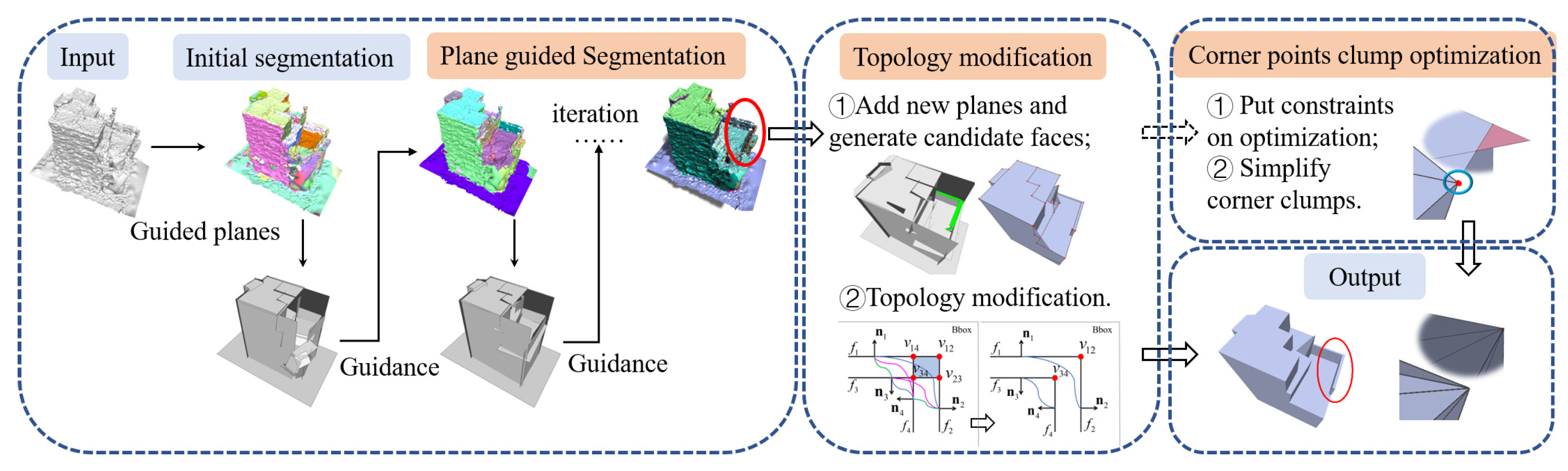
In summary, most of the current algorithms can remove noise on the surface of the model, but structure retention and restoration effects remain unsatisfactory. The feature classification method based on NVT is very sensitive to normal disturbances, and it is impossible to accurately classify feature points from a noisy model. Our goal is to classify feature points accurately, to preserve and restore the scene structure of the model when denoising, and to avoid introducing pseudo-features into the denoised model. More specifically, in this paper, we first apply joint bilateral filtering to the face normals using robust guidance normals; afterwards, we classify the feature points accurately by using the filtered facet normal; finally, we remove noise using anisotropic vertex denoising with a local geometric constraint to retain the scene structure features of the model and to avoid pseudo-features.

3. Methods

The algorithm divides the building model polygonization problem into four stages: (1) planar extraction based on plane-guided segmentation; (2) topology construction and topology optimization; (3) plane slicing and corner point clump optimization; and (4) polyhedron construction and output. The flow of the proposed method is shown in Figure 1.

3.1. Guided-Based Planar Segmentation

We use a joint constraint of distances and normals to extract the initial segmentation plane. When growth is based only on normals, the segmentation result is very sensitive to noise fluctuations on the surface, and smoothly transitioning angles are difficult to segment; by contrast, when growth is based only on distance, the segmented plane can flip over angles that do not belong to the plane and can cross the boundary, as shown in Figure 2d. Moreover, the front and back sides of the thin plate are divided into a plane area, as shown in Figure 2d. Therefore, we consider both distances and normals in the regional growth process so that the segmentation process is robust to noise.

Models reconstructed by photogrammetric processes inevitably have some surface defects, such as surface noise, local distortion, local deformations, and missing structures. Furthermore, the surface of a building model is usually covered with some small-scale structures, such as windows, balconies, air conditioning hangers, and tiles. These small-scale structures cause local uneven fluctuations in the plane structure. Defects and small-scale fluctuations in the model surface pose a challenge for planar segmentation. On the one hand, a strict distance threshold or normal threshold of segmentation results in too fine segmentation (oversegmentation) to obtain a concise and complete representation of the building plane, as shown in Figure 2b. On the other hand, this problem can be mitigated by increasing the normal angle threshold and distance threshold of the segmentation process. However, due to the limitations of traditional segmentation algorithms, this strategy leads to boundary crossing of the segmentation (undersegmentation) result, resulting in insufficient extraction of planes and incorrect topological connections between faces, as shown in Figure 2c.

To solve this problem, we propose a strategy of guided segmentation that first extracts an initial reliable plane as the seed plane; then iteratively guides segmentation, fusion, and merging through the plane; and finally extracts the plane corresponding to the final segmentation. The flow of the plane-guided segmentation method is shown in Figure 3. Our segmentation algorithm can be summarized as follows: (1) Initial segmentation—We refer to the segmentation algorithm of support agnostic Bayesian matching pursuit (SABMP); the difference is that we take two thresholds—the distance from the triangular face to the reference plane, and the normal angle between the triangular face and the reference plane—as the growth conditions. (2) Iterative segmentation—During segmentation, the plane corresponding to a large segmented area (the top $80\%$ sorted by area) is selected as the guide plane for segmentation in the next iteration. Then, among the mesh surfaces covered by these guide planes, we choose the triangular face with the smallest noise value as the initial growth surface; the noise value s of the triangular face is calculated with Equation (1), and the reference plane of the growth process is the current guide plane rather than a newly calculated plane every time it grows, until all the guide planes are traversed. (3) Fusion—Segmentation results containing fewer faces (less than the minimum number of segmentation faces) are fused to adjacent segmentation results with the closest normal, and the adjacent segmentation result that satisfies the normal constraint (default 20°, an empirical value summarized in our experiments) is fused to obtain the new plane segmentation result. (2) and (3) are iterated until the end of the process. (4) Segmentation merging—All segmentation results that are codirectional and coplanar (normal angle less than $\alpha 1$, the default for which is 20°) and close in distance (the default distance is less than $2\Delta \mathrm{d}$, and $\Delta \mathrm{d}=n·\overline{edge}$ is the distance threshold of segmentation, n is a factor of the average edge length, with the default value as 1) are merged; $\overline{edge}$ is the average edge length of the input mesh model. For details, please refer to Algorithm 1.

$$s=(1-|\cos \theta |)+\frac{dist\left(c_i,P\right)}{\Delta d}$$

(1)

where $\theta$ is the normal angle between the triangular face and the guided plane, $dist(c_i,P)$ is the distance from the center of mass $c_i$ of the triangular face $f_i$ to the plane P, and $\Delta d$ is the distance threshold of segmentation. The smaller the difference between the normal of the triangular plane and the plane (or the smaller the distance), the smaller the noise value.

For models with an unclear surface structure, when the segmentation threshold is set to a smaller value, more segmented planes are obtained, but the structural expression is fragmented and the overall structure is incomplete, as shown in Figure 3b; on the other hand, increasing the threshold can obtain concisely segmented planes, but details are inevitably lost, as shown in Figure 3c. Since the iterative process takes the guide plane as the reference, the growth process has a reliable and stable reference plane, which can better play a suitable guiding role, and the segmentation results of larger planes also affect the segmentation results of adjacent local small planes to finally obtain more concise and complete segmentation planes. The results of our guided segmentation model are shown in Figure 2e and Figure 3d.

Algorithm 1: Guided mesh plane segmentation framework.

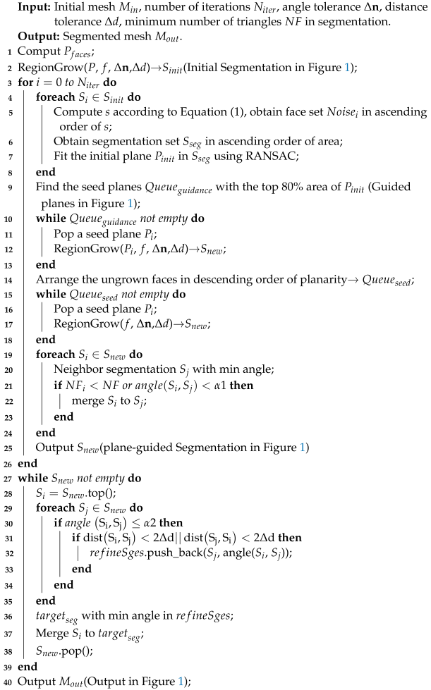
3.2. Topology Correction for Thin-Plate Structures

Based on building mesh polygonization (BMP) [11], according to the boundary adjacency relationship of the segmentation, we obtain the topological connection relationship of the segmentation plane, that is, the plane adjacency topological graph $\mathrm{G}$, which is composed of node $\mathrm{V}$ and the connection relationship $\mathrm{E}$ between two nodes $\mathrm{G}=(\mathrm{V},\mathrm{E})$. Among these, the centroid coordinates of the segmentation represent node $\mathrm{V}$ in the topological graph, and the connection between two adjacent nodes represents edge $\mathrm{E}$. However, narrow, flat, and thin regions in a building’s structure (called the thin-slab structure in this paper, such as the top surface of a child wall) are difficult to extract completely by the segmentation algorithm, as shown in Figure 4b, resulting in incorrect topological connections between the inner and outer planes of the thin plate.

Based on these considerations, we propose a topology correction scheme for the above problem. We consider the two planes as the inner and outer surfaces of the thin plate, and spatially they meet at a distance or fail to intersect, resulting in an incorrect or missing thin-plate structure (Figure 4c). Therefore, we propose correcting the incorrect topological relationship between the inner and outer planes of the thin plate by adding new planes; the detailed example is shown in Figure 5; here, our topological correction is applied only on the vertical thin plate.

Assuming that the segmentation of one side of the thin plate $S_p$ and the other side $S_q$ are connected in the topology graph, $S_p$ and $S_q$ must be adjacent to a common horizontal top surface, and there may be zero, one, or two common facades between $S_p$ and $S_q$. We optimize thin-plate topology by the following specific steps:

(1)

Regularization—Make a plane with a small area in $S_p$ and $S_q$ parallel to a plane with a large area, such as the thin-plate facade in Figure 5. The effect of regularization is shown in Figure 5, and regularization helps recover the structure of the thin plate.

(2)

Add a new top facade and define the topological relationship, as shown in Figure 5. First, we find the location of the new top surface. We obtain the smaller $Z_{max}$ of segmentation $S_p$ and $S_q$ through their bounding box (i.e., Bbox); then, if the $Z_{max}$ values of $S_p$ and $S_q$ are similar, we add a new plane $f_{aclinic}$ that is both adjacent and perpendicular to $S_p$ and $S_q$ in the topology diagram. If the $Z_{max}$ difference between $S_p$ and $S_q$ is large, it means that the elevations of the two facades are different, and a new plane $f_{aclinic}$ is added at the lower elevation position. Finally, we define the topological relationship of the added top surface. The added top surface $f_{aclinic}$ is adjacent to $S_p$ and $S_q$. If $S_p$ and $S_q$ have a common neighboring facade, then $f_{aclinic}$ should also be adjacent to their common facade, where the facade is the face that is nearly perpendicular to the ground.

(3)

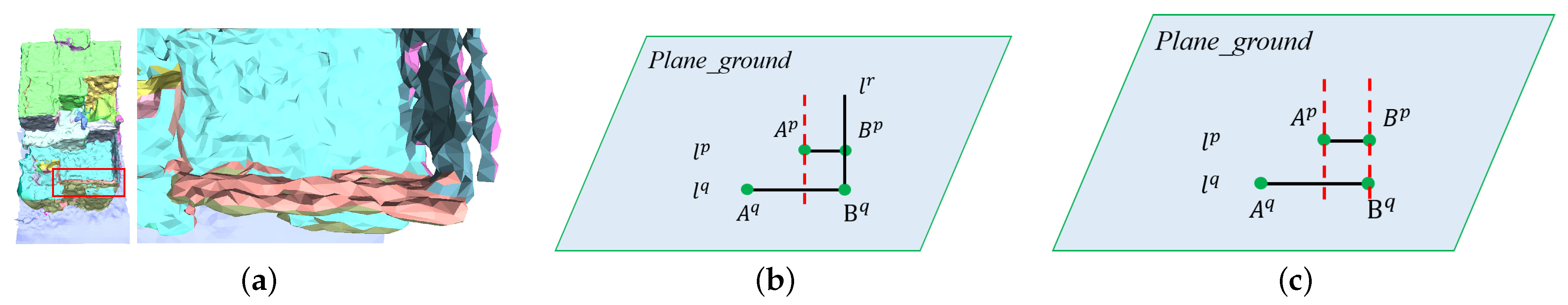
Add new side facades and define the topological relationship, as shown in Figure 5. Obtain the location of the new facade: we find the location of the new facade by a 2-dimensional projection. Specifically, we project the Bbox of $S_p$ and $S_q$ to the 2-dimensional ground $Plan{e}_{ground}$ to obtain line segments $l^p$ and $l^p$, and the two endpoints of the line segments are denoted as $A^p$, $B^p$ and $A^q$, $B^q$, as shown in Figure 6. There are two cases:

• Adding a new facade—If, in addition to $S_q$, the segmentation $S_p$ adjoins only one other segmentation $S_r$ or adjoins two facades with a distance less than $2{\overline{L}}_{\mathit{edge}}$, a new facade is needed. The Bbox of segmentation $S_r$$S_r$ is also projected onto $Pla{n}_{ground}$ to obtain the line segment $l^r$. If $A^p$ is the endpoint of line segment $l^p$ and is further away from line segment $l^r$, then the newly added elevation $f_{n1}$ will pass through endpoint $A^p$. Define the topology of $f_{n1}$: $f_{n1}$ as adjacent and perpendicular to the planes corresponding to $S_p$ and $S_q$; the 2-dimensional projection is represented by the red dashed segment in Figure 6b, while $f_{n1}$ is also adjacent and perpendicular to the top surface $f_{aclinic}$. Note that $f_{n1}$ is connected to the horizontal plane adjacent to the smaller segmentation in $S_p$ and $S_q$.
• Adding two new facades—If $S_p$ is not adjacent to any other facade except $S_p$, then two new facades are needed. The two new facades $f_{n1}$ and $f_{n2}$ pass through the endpoints $A^p$ and $B^p$. Define the topology of $f_{n1}$ and $f_{n2}$: $f_{n1}$ and $f_{n2}$ as adjacent and perpendicular to the plane in which $S_p$ and $S_q$ are located, and $f_{aclinic}$ is connected to the horizontal plane adjacent to the smaller segmented plane in $S_p$ and $S_q$. The 2-dimensional projection is represented by the red dashed segment in Figure 6c.

Topology of the added side facades: the newly added facade is adjacent to $S_p$ and $S_q$ and to their common nonfacade surfaces (the top and bottom adjacent faces).

(4)

Remove the incorrect topological connection of the reverse parallel facade present in a thin plate (the green connecting line in Figure 7b).

(5)

The coverage region of the newly added plane—In the segmented planes $S_p$ and $S_q$, triangles for which the distance from their center of mass to the newly added plane is within the specified range (the point-to-plane distance is less than $3{\overline{L}}_{edge}$ the average side length) belong to the covered triangles of this newly added plane.

(6)

Merge planes that are coplanar and codirectional.

(7)

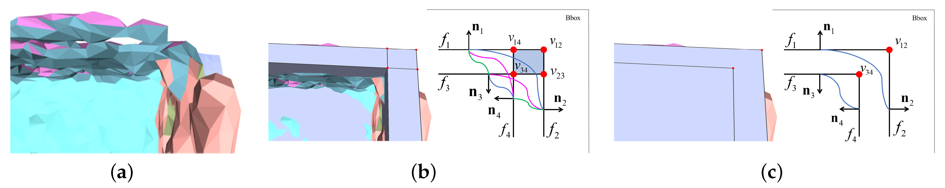
Topology correction of the inner and outer surfaces of the adjacent thin plates—Since it is difficult for the segmentation model to take into account thin and narrow areas existing in the building structure, the inner and outer surfaces of two adjacent thin plates are also connected incorrectly in the topology diagram, as indicated by the purple curve in Figure 7b. Figure 7b,c are 2D schematics of the local area of the thin plate in Figure 5, where the connection of facades $f_1$ and $f_4$ and $f_2$ and $f_3$ adds two new intersections $v_{1}4$ and $v_{2}3$, respectively. This adds a very small candidate surface at the corner of the thin-plate structure (the colored area of the 2D schematic in Figure 7b); however, this candidate surface is very easily lost in the optimization process, which eventually causes the thin-plate structure to be missing. In fact, in the actual building structure, $f_1$ and $f_4$ and $f_2$ and $f_3$ should not be connected. To solve this problem, we propose “topology correction of the inner and outer surfaces of a thin plate” to eliminate this kind of incorrect topology connection. Determination of the inner and outer facades of a thin plates: We intersect the center normal of the thin plate with the plane in which all the candidate surfaces are located. If the intersection point is inside the Bbox, then the plane is the inner surface of the thin plate; if there is no intersection point or the intersection point is outside the Bbox, then the plane is the outer surface. According to the geometric rules of the actual building structure, we stipulate that the inner and outer surfaces of the thin plate are not connected to each other, so the incorrect topological connections (the purple connections in Figure 7b) between the inner and outer $f_1$ and $f_4$ and $f_2$ and $f_3$ of the thin plate are eliminated, as shown in Figure 7c. The top of the thin plate is not cut into multiple small areas, which makes it more likely that the thin plate structure will not be lost during optimization.

By regularizing the thin-plate facade, adding new planes (fixing the thin-plate topological connections), and eliminating the incorrect topological connections of the thin plate, the topological relationships between the inner and outer surfaces of the thin-plate structure are correctly constructed, and the thin-plate structure of the polygonal model is completely reconstructed, as shown in Figure 5.

3.3. Corner Point Clump Optimization and Polyhedron Construction

Three extracted adjacent planes form an intersection. However, abstract/approximate planes do not necessarily strictly intersect at the same intersection position when the number of adjacent planes is greater than three. When $n(n>3)$ adjacent planes intersect, there are $C_n^3$ intersection points, each plane will intersect $C_{n-1}^2$ times with $C_{n-1}^2$ intersection points, and there are $C_n^3-C_{n-1}^2$ intersection points not in the current plane. Since the surface of the model reconstructed based on MVS is not exactly flat, and the segmentation area may contain some detailed structures, it is difficult for extracted planes with larger areas to fully and truly express the geometric orientation of the covered surface. The location of the extracted planes is not realistic and not close enough to fit the real building surface, which eventually leads to multiple redundant corner points and reduces geometric expression accuracy. Taking the intersection of four adjacent planes as an example, in the corner at the top of the house in Figure 8, every three planes intersect to form one intersection point, and there are four intersections at the top corner of the house, as shown in Figure 8b.

PolyFit [10] and SABMP [11] form polygons from intersection points and intersection lines after the planes are intersected and then obtain the preserved closed-flow polygonal model through optimization. However, these methods do not consider redundant intersection points. On the one hand, redundant polygons or triangles composed of redundant intersection points may appear after optimization, as shown in Figure 8c and Figure 9d; on the other hand, the resulting model of polygonization can have redundant corner points, such as the corners in Figure 8c and Figure 9d. In addition, the fidelity of the polygonal model to represent the original surface needs to be improved. We would like to concurrently simplify the resultant polygon model and improve model representation accuracy.

To solve the above problem, we propose a two-step strategy based on “corner point clumps”. We define all intersections $I_i,I_j,\cdots$ of the $n(n>3)$ planes that correspond to segmented planes $S_1,S_2,\cdots ,S_n$ (any one of them is adjacent to the others) as belonging to a corner point clump $C\left(I_i,I_j,\cdots \right)$, as shown in the blue circles in Figure 8b, where there are four corner point clumps. The two-step strategy based on “corner point clumps” is as follows:

In the first step, constraints are imposed on the optimized result to avoid redundant triangles/polygons at the corners. In the candidate surface selection stage, a new constraint term is added: if the polygon candidate plane $f_i$ satisfies Equation (2), then the plane is deleted ($x_i=0$); $I\left(f_i\right)$ denotes all constituent intersections of the candidate plane $f_i$, and Equation (2) represents the case when all constituent intersections of a candidate plane belong to the same corner point group, as shown in the red polygon/triangle in Figure 8b, in which case the candidate face should be deleted. All formulas used in the optimization are specified in Appendix A.

$$x_i=0,\forall I\left(f_i\right)\in C\left(I_i,I_j,\cdots \right)$$

(2)

In the second step, simplification of the corner point clusters is implemented. On the premise of ensuring geometric accuracy, multiple intersection points that remain in the corner point clumps are merged, while redundant corner points are removed. We hope that the candidate polygons after intersection merging are better fitted to the surface of the original mesh and improve the accuracy of the model. Ideally, only one intersection point is retained in a corner point clump, but we do not do this if the accuracy decreases after the intersection points are merged. For the two intersection points retained in the same corner point cluster that can form an edge, we merge them using a method similar to edge collapse. The intersection points have some reliability because they are obtained from the intersection of the extracted planes, so we use either one of them as a retained point during edge collapse. The cost of collapsing from intersection $I_i$ to intersection $I_j$ is calculated according to Equation (3).

$$E_{\left(I_i,I_j\right)}=\sum _{n=1}^{N{F}_{I_i}}\sum _{m=1}^{V_n}{d}_{mn}^i$$

(3)

where $N{F}_{I_i}$ is the set of candidate planes adjacent to intersection $I_i$, $V_n$ is the set of all vertices of the nth candidate planes in $N{F}_{I_i}$ covering the original region, and $d_{mn}^i$ is the distance from vertex m to its corresponding candidate plane n. Suppose intersection $I_i$ collapses to intersection $I_j$. We calculate the cost $E_{\left(I_i,I_j\right)}$ before the edge collapse operation and the cost $E_{\left(I_i,I_j\right)}^{\prime }$ after the simulated edge collapse operation. If $E_{\left(I_i,I_j\right)}<E_{\left(I_i,I_j\right)}^{\prime }$ (the cost decreases after edge collapse), which means the distance between the polygonal model and the original surface decreases and the geometric accuracy improves after processing, then intersection $I_i$ is allowed to collapse to intersection $I_j$. Conversely, the same strategy is used to simulate the collapse of intersection $I_j$ to intersection $I_i$ until all redundant intersections within the corner point clump are visited; the result of corner point clump optimization is shown in Figure 8d. When the vertex positions of the planar polygons are changed, the original planar polygon may become two polygons that are not coplanar, and new triangles may be generated in this process, but the accuracy of the final model will be improved, and the number of intersection points will be reduced due to the constraint of Equation (3). As shown in Figure 8, the unoptimized RMS (%Bbox ) in Figure 8c is 0.006279, and the RMS (%Bbox ) of our optimized result in Figure 8d is 0.00558.

4. Results

To verify the effectiveness of the algorithm, we applied it to a large number of artificial building mesh models, including the SUM [39] dataset of real-scene models based on image reconstruction, Nanyang data, Shenyang data, Ningbo data and the Villa model, noisy surfaces with (House_a, House_b, and Cottage), and the real-scene model Barn reconstructed by laser point clouds.

4.1. Qualitative Assessment Experiments

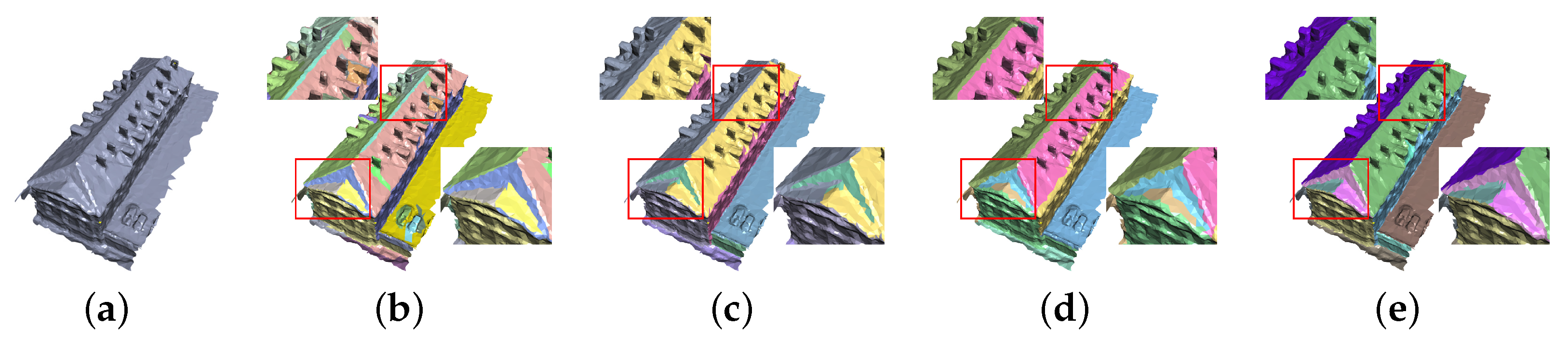
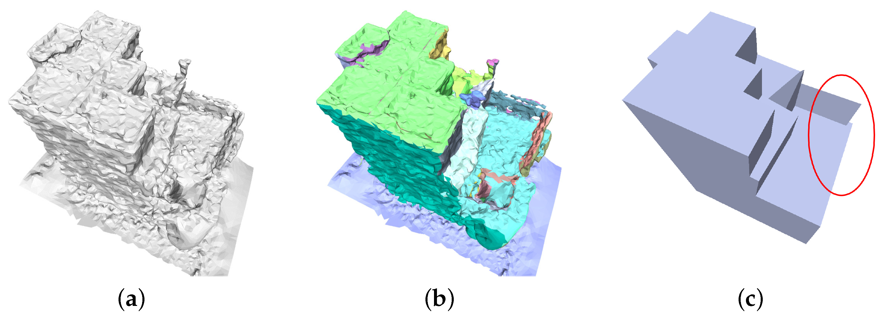
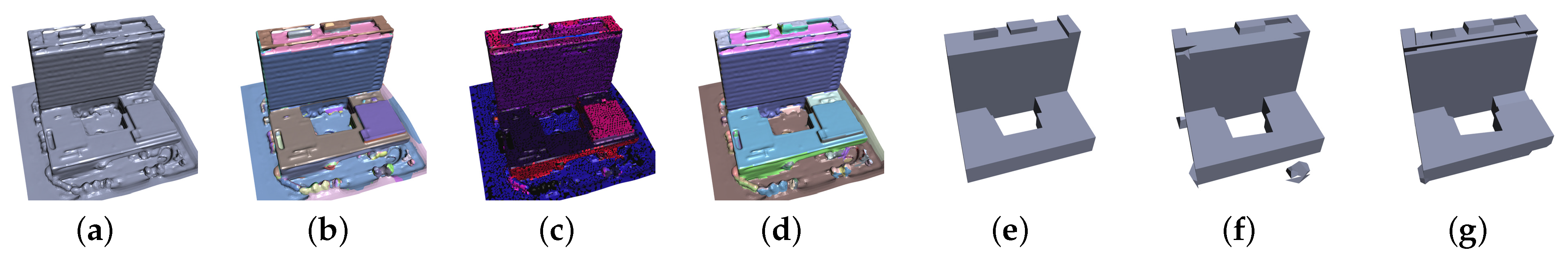
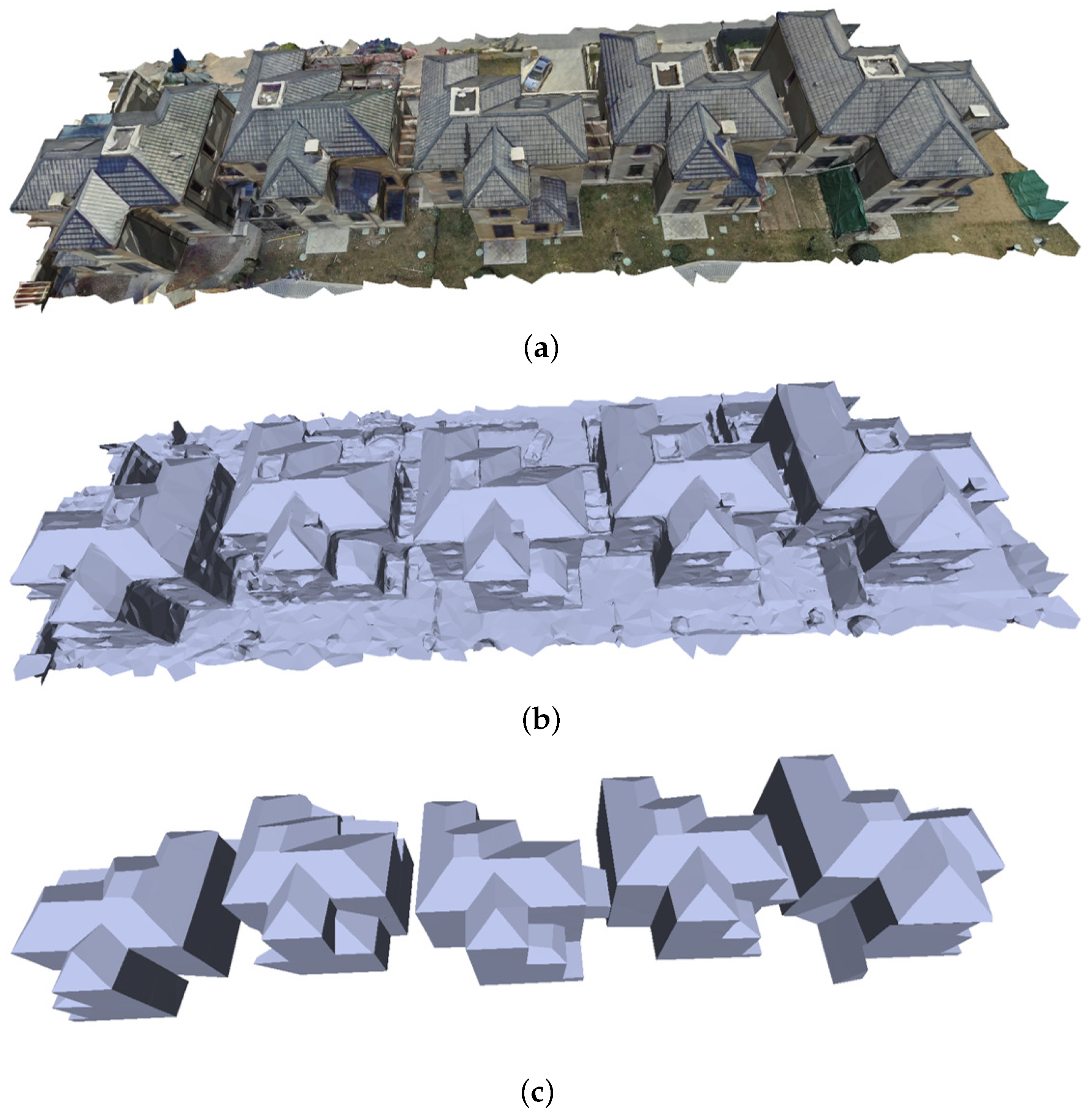
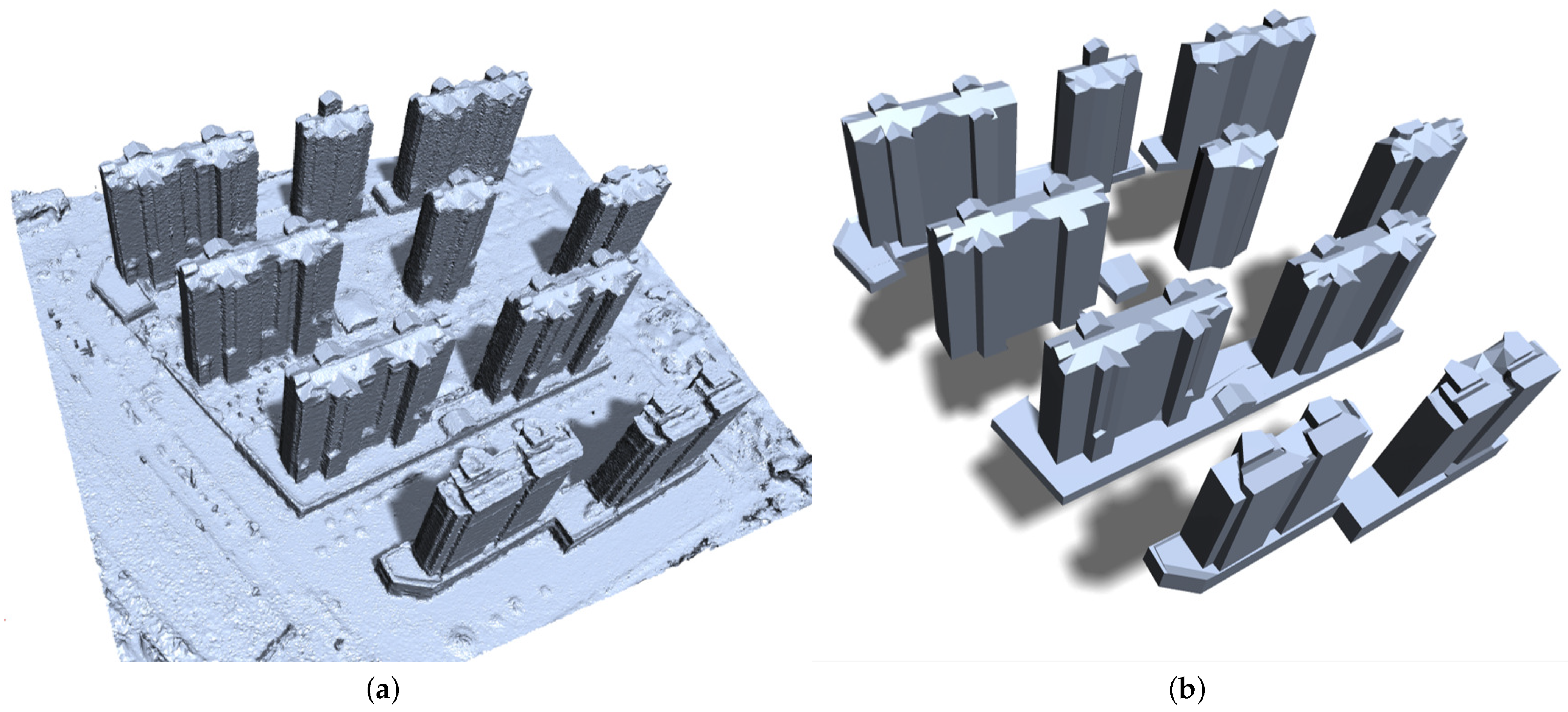
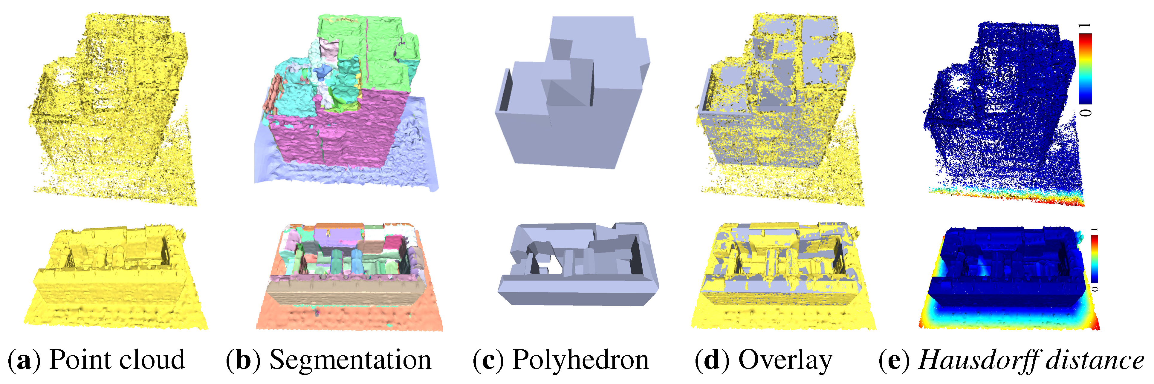
4.1.1. Qualitative Comparison of the Segmentation and Polyhedral Results

Figure 10 shows the comparison of the planar segmentation results. Comparing our segmentation results with those of SABMP [11] (Figure 10) and the model without the plane-guided strategy (Figure 10c), it can be seen that these segmentation results are the optimal results among multiple groups of parameters. The segmentation results of SABMP [11] cross prismatic edges, as shown in Figure 10b. This is because SABMP considers only the distance and not the normal value when growing regions. Segmentation methods without guided planes work well for models with simple structures, such as the Barn model. However, plane extraction is incomplete for noisy or complex models, such as Nanyang_3 and Nanyang_5 in Figure 10c; this is because the segmentation algorithm is not robust to model surface defects and is easily affected by fluctuations in face normals and vertex positions. In contrast, our planar segmentation boundary is more accurate, clear, and straight, and the segmented planar extraction results are more prominent, as shown in Figure 10d.

4.1.2. Qualitative Comparison of Structure-Aware Results

Structural perceptibility: To better reveal the visual quality of the reconstructed building models, we demonstrate a number of individual buildings in Figure 10 and Figure 11. From these visual results, we can see that our approach succeeds in obtaining visually plausible reconstructions despite the buildings having different structures/styles and the input mesh models having different densities and different levels of noise. In the comparison of simplifications, we keep the number of vertices or triangles unchanged and use QEM [17] and ACVD [21] to simplify models, as shown in Figure 11b,c. Compare to the results of QEM [17] and ACVD [21], we can see that the planar and linear structures of buildings are more prominent and more structurally aware in our building models. In addition, Figure 10 shows that our method extracts more building details compared to SABMP [11], and structural perceptiveness is improved.

Thin plates: SABMP [11] does not consider vertical thin-slab structures such as child walls and fences. Due to the limitation of the segmentation method, the planes of such structures cannot be properly extracted, as shown in Figure 11b. Our proposed plane-guided segmentation method distinguishes the two sides of a thin-plate structure well, and combined with the topology optimization strategy in this paper, the thin-slab structure of the polyhedral building model is effectively recovered, as shown in Figure 12d. Note that for Shenyang_a in Figure 12, its polygonization process successfully reconstructs the narrow thin-plate enclosure without a topology optimization strategy because the segmentation results accurately extract the top plane of the thin-plate structure.

Corner points: Comparison of the optimization results with respect to corner point clumps is shown in Figure 9, where we compare our results with those of SABMP. A comparison between Figure 9d,e shows that the corner points are more streamlined, and the geometric connections are closer to the real structure in our building model reconstruction. With optimization of the corner point clusters, our model can express multiple (greater than three) planes adjacent to the corner structure using only one vertex.

In contrast to other improved methods, such as Li’s method [9] due to the use of the “1-ring patch model”, some elongated or narrow structures are ignored in the plane extraction process, as shown in Figure 13c,f. By contrast, our segmentation results can extract these narrow planes and build them successfully in the polygonal model, as shown at the top of the model in Figure 13g.

In addition, we have used our approach for polyhedral structured modeling in a range of building groups. As shown in Figure 14 and Figure 15, these buildings are modeled as polyhedrons independently. In Figure 14, the original model has 18,436 vertices and 36,559 triangles, and after simplification, the number of vertices is 2070, the number of faces is 4124, and the simplification ratios of vertices and triangular faces are 88.77% and 88.72%, respectively. In Figure 15, the original mesh model has 806,198 vertices and 1,609,613 triangles. After simplification, the number of vertices is 2817, the number of faces is 5364, and the simplification ratios of vertices and triangular faces are 99.65% and 99.67%, respectively. Figure 15 shows that the roof structure of the building in the simplified model is more prominent, the roof ridge line in Figure 14 is clear and straight, and the model has higher geometric accuracy; thus, the improved method we propose has better structure perception ability.

4.2. Quantitative Evaluation Experiments

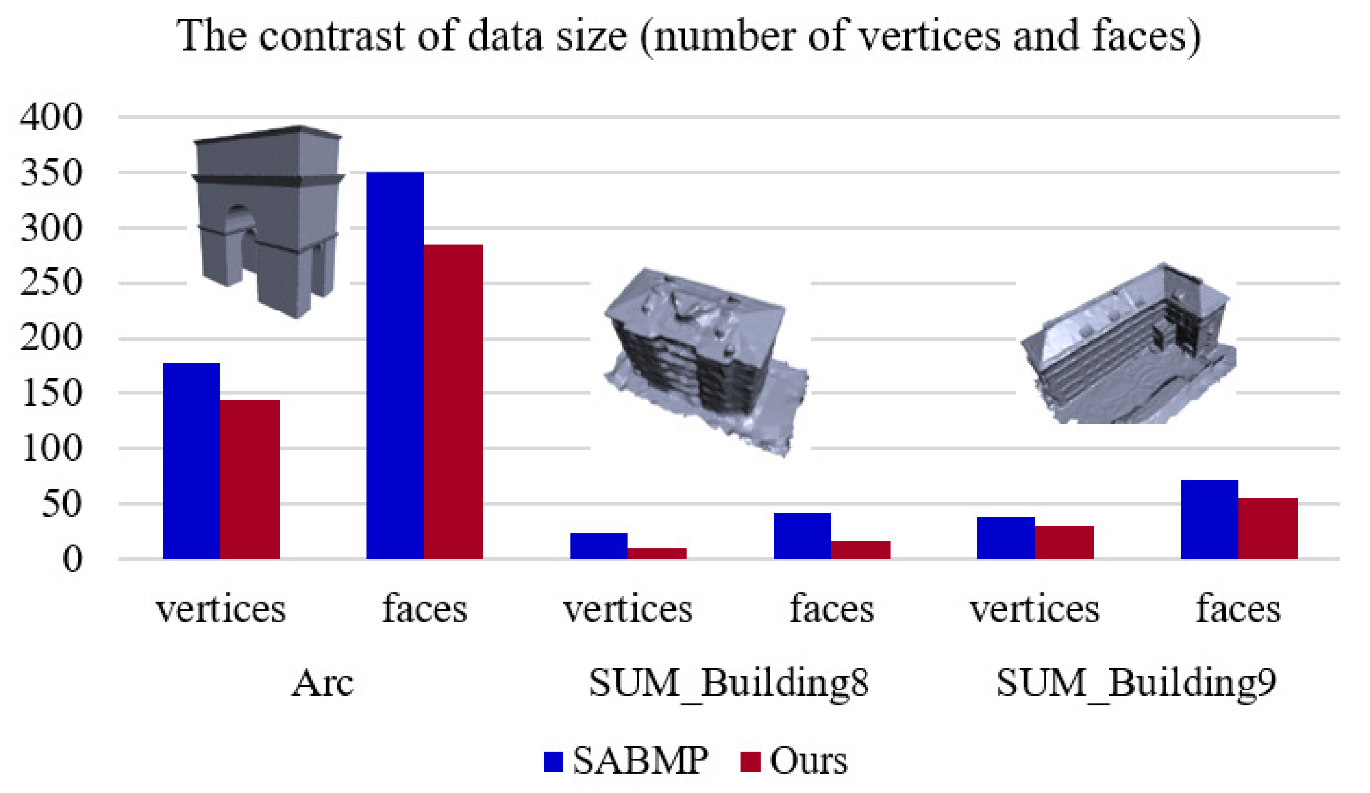
4.2.1. Quantitative Comparison of the Number of Planes and Simplification Capability

To concretely quantify the polygonal models generated by our segmentation algorithm, we analyze the improvement of our method in terms of the number of extracted planes, and comparison between the output model and the input model in terms of the amount of data, as shown in

Table 1. Information about the simplified polygonal meshes. The polygonal meshes have been previously triangulated for visualization.

Model	Input Vertices	Input Faces	Planes	SABMP [11]		Time (s)	Planes	Ours		Time (s)
				Output Vertices	Output Faces			Output Points	Output Faces
SUM _ Building1	15,383	30,143	64	43	82	5.7	55	121	238	27.35
College	33,845	65,614	84	156	308	82.2	93	647	1290	267
Nanyang _ 3	44,380	88,271	93	89	170	12	57	221	438	14.32
House _ b	18,716	37,245	65	52	100	21.3	42	93	162	65.3
Arc	13,631	27,258	75	177	350	3.4	71	144	284	12
SUM _ Building8	3321	6503	37	23	42	1.2	14	10	16	15.6
SUM _ Building9	6295	12,414	47	38	72	0.71	22	30	56	16.5

. Our model segments fewer planes, but as seen in Figure 10, Figure 12 and Figure 13, our plane-guided segmentation method adequately reconstructs models; therefore, segmentation by our method is more concise and complete. Our guided-based planar segmentation algorithm makes full use of the extracted plane information and uses a reliable geometric plane as a guide to integrate noisy and small structures into the corresponding plane during segmentation, so it can obtain a more complete, concise, and reliable segmented plane.

Furthermore, our building simplification results have a smaller amount of data due to corner point clumps, as seen from Table 1. For the models with corner clumps in processing (Figure 9), their output vertex number and output triangular surface number are reduced compared with the results of SABMP [11], as shown in Figure 16, and the figure shows that our corner point clump algorithm works well in simplifying models.

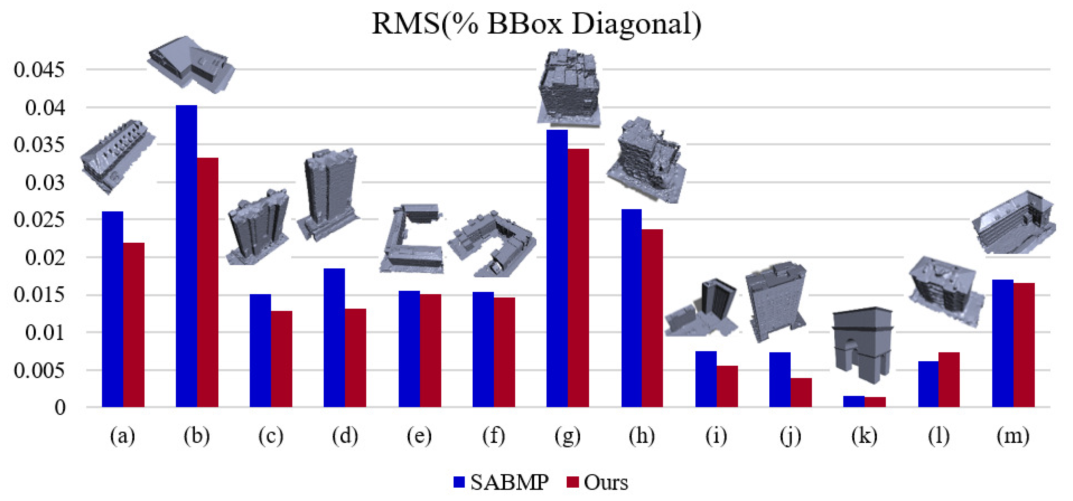
4.2.2. Quantitative Comparison of Geometric Accuracy

Geometric accuracy is a key metric for evaluating the results and expressing the accuracy of polygon models. We evaluate the closeness of our simplified model to the original model by calculating the Hausdorff distance between the two meshes [40], and we calculate the RMS (values with respect to the BBox diagonal) of the polygonal model to the original mesh surface; the results are shown in Figure 17 and Figure 18. Figure 17 compares our method with SABMP [11], using the model results shown in Figure 9, Figure 10 and Figure 12.

For general models without topology correction and corner-point optimization, the geometric accuracy of our building model is essentially higher than that of SABMP [11]. As seen in Figure 17 and Figure 18, the vertices, edges, and faces of our polyhedral results are closer to those of the original surfaces. There are two reasons for this: first, due to our plane extraction step, plane guidance is performed by iteration, and we make full use of plane information during segmentation. The obtained plane structure is more consistent with the original representation, and small planar structures can be extracted, but the plane extraction results are not too finely divided, as shown in Figure 13 and Figure 17; second, using the dual constraints of distance and normal values during segmentation makes the boundary of the segmentation region more accurate; thus, the geometric position of the fitted plane is more accurate.

For building models with thin-plate structures, our polyhedral results also have higher structural accuracy than SABMP [11], as shown in Figure 17 and Figure 18. The reason for this, in addition to the segmentation approach mentioned above, is that thin-slab structures at a certain scale can be recovered accurately by our proposed thin-plate topology correction scheme, as shown in Figure 12. The recovery of small-scale thin-plate structures further improves the geometric accuracy of models.

For buildings with multiple (greater than three) adjacent planes, our polyhedral models mostly have higher structural accuracy than that of SABMP [11], as shown in Figure 17 and Figure 18. The reason is not only due to the abovementioned segmentation, but also because of our corner point clump optimization strategy. On the one hand, by imposing constraints on the optimization process, erroneous candidate faces can be eliminated, and on the other hand, such corner structures can be simplified on the premise of improving the closeness to the original surface, as shown in Figure 9. The exception is the SUM_Building8 data; our polyhedron has more concise results, and the results of SABMP [11], although closer to the original surface, perform poorly in terms of regularity. Combined with Figure 16, it can be seen that our results not only simplify the corner point clumps but also improve the accuracy of the model and increase the realism of the representation while reducing the amount of data.

The result of superimposing with the original point cloud is shown in Figure 19. The point cloud in the first row is a noisy, dense point cloud generated by photogrammetry based on images, and the point cloud in the second row is a clean point cloud generated by laser scanning. Superimposing the point clouds and the polyhedral models illustrates the accuracy of the reconstructed model. The Hausdorff distance also shows that our polyhedral model can more completely retain the structural parts of buildings, and the areas with larger errors are basically found at the edges where there is no structure.

4.2.3. Quantitative Comparison of Run Times

Table 1 provides the running-time comparison for the examples shown on a PC with an Intel Core i7-8550U CPU. It can be seen that our method is less efficient than SABMP [11] in dealing with most models. There are three reasons for this: first, our method adds a plane as a guide during segmentation, and the time consumption of iterative segmentation increases with the number of iterations; second, we add a topology optimization step in the topology construction, and this topology repair process also increases the reconstruction time if there is a thin-plate structure in the model; third, we add corner point clumps in the simplification step, which also increases time consumption when simplifying the model.

4.3. Discussion

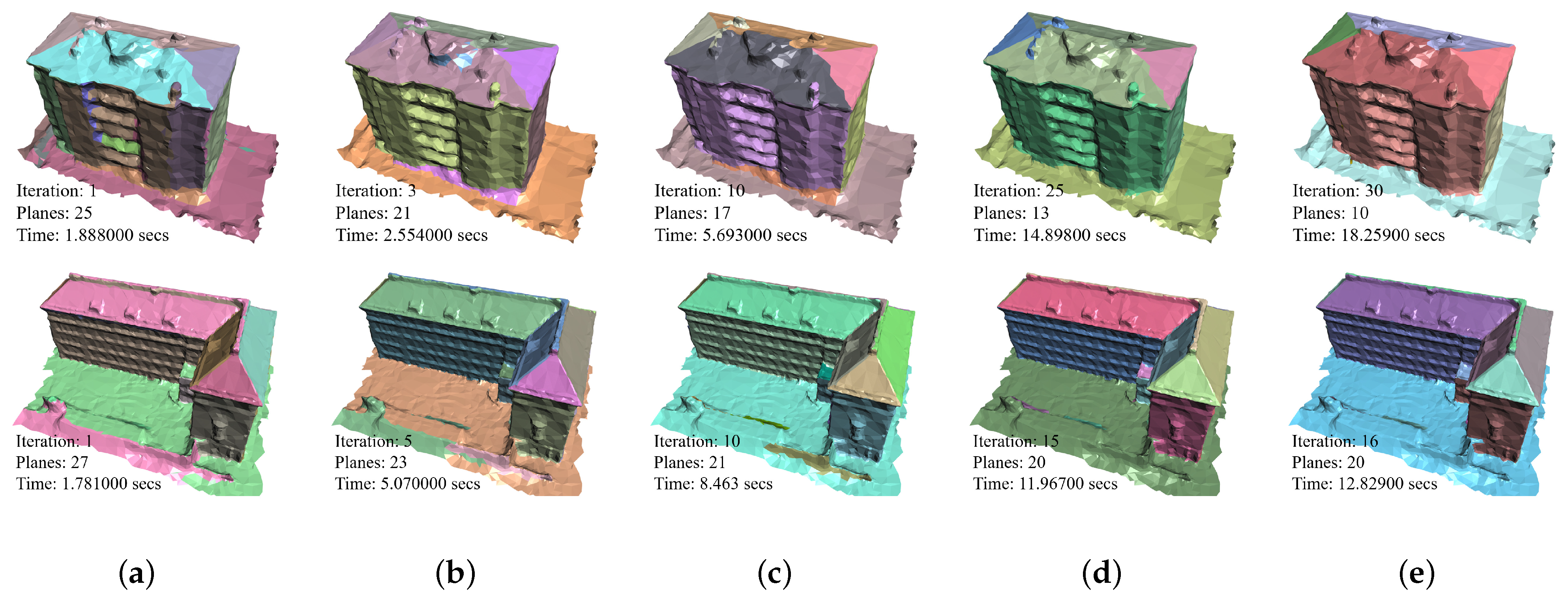
4.3.1. Influence of the Iteration Number on Segmentation

The influence of the number of plane-guided iterations on the segmentation results is discussed in this section. For example, we analyze the SUM_Building8 model with large surface fluctuations and the SUM_Building9 model with a flat surface. The number of iterations, the number of segmentation results, and the segmentation time are listed in the lower left corner of Figure 20. With other parameters fixed, the number of segmentation planes decreases when the number of plane guidance iterations increases, and the planar segmentation results are more streamlined. After a certain number of iterations, the number of planes and the segmentation results tend to stabilize. On this basis, the number of iterations continues to increase, and the number of planes and segmentation results rarely change. The same situation occurs on the SUM_Building9 model with a flat surface, the difference being that the optimal number of iterations is less for the clean model. In addition, we found that the number of segmentation planes gradually decreases with the number of iterations and stabilizes after a certain number of iterations, and the segmentation results are also more desirable. Since segmentation time increases linearly with the number of iterative guided-based planar segmentation operations, a higher number of iterations theoretically leads to a more desirable segmentation result. However, this increases time consumption. Therefore, the number of iterations should be reduced as much as possible while maintaining stable segmentation results.

4.3.2. Limitations

Our method can obtain more accurate segmentation results, recover thin-plate structures, and obtain fine polygonal models. However, the algorithm still has several limitations that need to be addressed: (1) Execution efficiency needs to be improved. Iterative segmentation, topology optimization, and corner point clump processing all slow processing to some extent, even though they allow the model to achieve better visual effects or higher accuracy. (2) Parameter settings are not automated. The number of plane-guided segmentation steps and segmentation thresholds need to be set according to the model, which is not smart enough. For segmentation, the parameter setting depends on the noise level of the building surface and the complexity of the building structure. The more complex the structure, the finer the segmentation needed; then, the threshold of segmentation needs to be stricter to some extent, and the number of iterations increases with the surface noisiness. (3) Since the planes intersect based on topological connections, the ideal polyhedral model may not be obtained when dealing with buildings that lack geometric information (e.g., missing facades or floors).

5. Conclusions

In this paper, we propose three improvements to SABMP [11] and present a polygonal construction method based on planar guidance, topological repair, and corner point optimization. Its improvements mainly consists of three parts: A segmentation technique based on guided planes, thin-plate topology repair, and polyhedron construction based on corner-point clump optimization. From the quantitative analysis, in terms of geometric accuracy, our results reduce the distance error by up to 46.61% compared with SABMP [11] before optimization, which is consistent with the visual comparison results in the qualitative analysis. In terms of being lightweight, our building polyhedral results have a high simplification ratio of up to 99.67% for building complexes. For most models, our results are more data-intensive than SABMP [11] due to the more richly detailed structure. However, for buildings with corner point clump structures, our results have up to 61.90% fewer triangular faces than SABMP [11]. In general, comparing SABMP [11] with the current simplification algorithm, this paper achieves the following four goals: (1) improves the region growth segmentation algorithm, which improves the accuracy and completeness of plane extraction; (2) restores the thin-plate structure of a building; (3) simplifies corner point expression, which improves the realism and geometric accuracy of the polygonal model; and (4) preserves more details of the polygonal model and enhances the structural awareness of the polygonal model construction algorithm.

References

1. Westoby, M.J.; Brasington, J.; Glasser, N.F.; Hambrey, M.J.; Reynolds, J.M. Structure-from-motion’photogrammetry: A low-cost, effective tool for geoscience applications. Geomorphology 2012, 179, 300–314. [Google Scholar] [CrossRef]
2. Seitz, S.M.; Curless, B.; Diebel, J.; Scharstein, D.; Szeliski, R. A comparison and evaluation of multi-view stereo reconstruction algorithms. In Proceedings of the 2006 IEEE Computer Society Conference on Computer Vision and Pattern Recognition (CVPR’06), New York, NY, USA, 17–22 June 2006; Volume 1, pp. 519–528. [Google Scholar]
3. Ziegel, E.R.; Fotheringham, S.; Rogerson, P. Spatial Analysis and GIS. Technometrics 1997, 39, 238. [Google Scholar] [CrossRef]
4. Verdie, Y.; Lafarge, F.; Alliez, P. LOD Generation for Urban Scenes. ACM Trans. Graph. 2015, 34, 1–14. [Google Scholar] [CrossRef]
5. Li, M.; Rottensteiner, F.; Heipke, C. Modelling of buildings from aerial LiDAR point clouds using TINs and label maps. ISPRS J. Photogramm. Remote Sens. 2019, 154, 127–138. [Google Scholar] [CrossRef]
6. Han, J.; Zhu, L.; Gao, X.; Hu, Z.; Zhou, L.; Liu, H.; Shen, S. Urban Scene LOD Vectorized Modeling from Photogrammetry Meshes. IEEE Trans. Image Process. 2021, 30, 7458–7471. [Google Scholar] [CrossRef]
7. Li, M.; Wonka, P.; Nan, L. Manhattan-World Urban Reconstruction from Point Clouds. In Proceedings of the European Conference on Computer Vision, Amsterdam, The Netherlands, 11–14 October 2016; Springer: Berlin/Heidelberg, Germany, 2016; pp. 54–69. [Google Scholar] [CrossRef]
8. Fang, H.; Lafarge, F. Connect-and-slice: An hybrid approach for reconstructing 3d objects. In Proceedings of the IEEE/CVF Conference on Computer Vision and Pattern Recognition, Seattle, WA, USA, 14–19 June 2020; p. 13. [Google Scholar]
9. Yan, L.; Li, Y.; Xie, H. Urban Building Mesh Polygonization Based on 1-Ring Patch and Topology Optimization. Remote Sens. 2021, 13, 4777. [Google Scholar] [CrossRef]
10. Nan, L.; Wonka, P. Polyfit: Polygonal surface reconstruction from point clouds. In Proceedings of the IEEE International Conference on Computer Vision, Venice, Italy, 22–29 October 2017; pp. 2353–2361. [Google Scholar]
11. Bouzas, V.; Ledoux, H.; Nan, L. Structure-aware building mesh polygonization. ISPRS J. Photogramm. Remote Sens. 2020, 167, 432–442. [Google Scholar] [CrossRef]
12. Chen, Z.; Khademi, S.; Ledoux, H.; Nan, L. Reconstructing compact building models from point clouds using deep implicit fields. arXiv 2021, arXiv:2112.13142. [Google Scholar]
13. Nauata, N.; Chang, K.-H.; Cheng, C.-Y.; Mori, G.; Furukawa, Y. House-GAN: Relational Generative Adversarial Networks for Graph-Constrained House Layout Generation. In Proceedings of the European Conference on Computer Vision, Munich, Germany, 8–14 September 2020; Springer: Berlin/Heidelberg, Germany, 2020; pp. 162–177. [Google Scholar] [CrossRef]
14. Qian, Y.; Zhang, H.; Furukawa, Y. Roof-gan: Learning to generate roof geometry and relations for residential houses. In Proceedings of the IEEE/CVF Conference on Computer Vision and Pattern Recognition, Nashville, TN, USA, 20–25 June 2021; pp. 2796–2805. [Google Scholar]
15. Gui, S.; Qin, R. Automated LoD-2 model reconstruction from very-high-resolution satellite-derived digital surface model and orthophoto. ISPRS J. Photogramm. Remote Sens. 2021, 181, 1–19. [Google Scholar] [CrossRef]
16. Wang, J.; Hu, X.; Meng, Q.; Zhang, L.; Wang, C.; Liu, X.; Zhao, M. Developing a Method to Extract Building 3D Information from GF-7 Data. Remote Sens. 2021, 13, 4532. [Google Scholar] [CrossRef]
17. Garland, M.; Heckbert, P.S. Surface simplification using quadric error metrics. In Proceedings of the 24th Annual Conference on Computer Graphics and Interactive Techniques, Los Angeles, CA, USA, 1 October 1997; pp. 209–216. [Google Scholar]
18. Melax, S. A simple, fast, and effective polygon reduction algorithm. Game Dev. 1988, 11, 44–49. [Google Scholar]
19. Li, M.; Nan, L. Feature-preserving 3D mesh simplification for urban buildings. ISPRS J. Photogramm. Remote Sens. 2021, 173, 135–150. [Google Scholar] [CrossRef]
20. Cohen-Steiner, D.; Alliez, P.; Desbrun, M. Variational shape approximation. ACM Trans. Graph. 2004, 23, 905–914. [Google Scholar] [CrossRef]
21. Lévy, B.; Liu, Y. Lp centroidal voronoi tessellation and its applications. ACM Trans. Graph. (TOG) 2010, 29, 1–11. [Google Scholar] [CrossRef]
22. Lévy, B.; Bonneel, N. Variational Anisotropic Surface Meshing with Voronoi Parallel Linear Enumeration. In Proceedings of the 21st International Meshing Roundtable, San Jose, CA, USA, 7–10 October 2012; Springer: Berlin/Heidelberg, Germany, 2013. [Google Scholar] [CrossRef]
23. Bauchet, J.-P.; Lafarge, F. City reconstruction from airborne lidar: A computational geometry approach. In Proceedings of the 3D GeoInfo 2019-14thConference 3D GeoInfo, Singapore, 24–27 September 2019. [Google Scholar]
24. LeDoux, H.; Ohori, K.A.; Kumar, K.; Dukai, B.; Labetski, A.; Vitalis, S. CityJSON: A compact and easy-to-use encoding of the CityGML data model. Open Geospat. Data, Softw. Stand. 2019, 4, 1–12. [Google Scholar] [CrossRef]
25. Gröger, G.; Kolbe, T.H.; Nagel, C.; Häfele, K.-H. Ogc City Geography Markup Language (Citygml) Encoding Standard; Open Geospatial Consortium: Rockville, MD, USA, 2012. [Google Scholar]
26. Zhu, L.; Shen, S.; Gao, X.; Hu, Z. Large scale urban scene modeling from mvs meshes. In Proceedings of the European Conference on Computer Vision (ECCV), Munich, Germany, 8–14 September 2018; pp. 614–629. [Google Scholar]
27. Zhu, L.; Shen, S.; Hu, L.; Hu, Z. Variational building modeling from urban mvs meshes. In Proceedings of the 2017 International Conference on 3D Vision (3DV), Qingdao, China, 10–12 October 2017; pp. 318–326. [Google Scholar]
28. Li, M.L.; Nan, L.L.; Smith, N.; Wonka, P. Reconstructing building mass models from UAV images. Comput. Graph. 2016, 54, 84–93. [Google Scholar] [CrossRef]
29. Zhang, F.; Nauata, N.; Furukawa, Y. Conv-MPN: Convolutional Message Passing Neural Network for Structured Outdoor Architecture Reconstruction. In Proceedings of the IEEE/CVF Conference on Computer Vision and Pattern Recognition, Seattle, WA, USA, 13–19 June 2020; pp. 2795–2804. [Google Scholar] [CrossRef]
30. Schnabel, R.; Wahl, R.; Klein, R. Efficient RANSAC for point-cloud shape detection. In Computer Graphics Forum; Blackwell Publishing Ltd.: Oxford, UK, 2007; pp. 214–226. [Google Scholar]
31. Lafarge, F.; Mallet, C. Creating Large-Scale City Models from 3D-Point Clouds: A Robust Approach with Hybrid Representation. Int. J. Comput. Vis. 2012, 99, 69–85. [Google Scholar] [CrossRef]
32. Oesau, S.; Lafarge, F.; Alliez, P. Planar Shape Detection and Regularization in Tandem. Comput. Graph. Forum 2015, 35, 203–215. [Google Scholar] [CrossRef] [Green Version]
33. Fang, H.; Lafarge, F.; Desbrun, M. Planar shape detection at structural scales. In Proceedings of the IEEE Conference on Computer Vision and Pattern Recognition, Salt Lake City, UT, USA, 18–23 June 2018; pp. 2965–2973. [Google Scholar]
34. Guinard, S.; Landrieu, L.; Caraffa, L.; Vallet, B. Piecewise-Planar Approximation of Large 3d Data as Graph-Structured Optimization. ISPRS Ann. Photogramm. Remote Sens. Spat. Inf. Sci. 2015, V-2/W5, 365–372. [Google Scholar] [CrossRef]
35. Zhu, X.; Liu, X.; Zhang, Y.; Wan, Y.; Duan, Y. Robust 3-D Plane Segmentation from Airborne Point Clouds Based on Quasi-A-Contrario Theory. IEEE J. Sel. Top. Appl. Earth Obs. Remote Sens. 2021, 14, 7133–7147. [Google Scholar] [CrossRef]
36. Mehra, R.; Zhou, Q.; Long, J.; Sheffer, A.; Gooch, A.; Mitra, N.J. Abstraction of man-made shapes. In Proceedings of the ACM SIGGRAPH Asia 2009 Papers, Yokohama, Japan, 16–19 December 2009; pp. 1–10. [Google Scholar]
37. Boykov, Y.; Kolmogorov, V. An experimental comparison of min-cut/max- flow algorithms for energy minimization in vision. IEEE Trans. Pattern Anal. Mach. Intell. 2004, 26, 1124–1137. [Google Scholar] [CrossRef] [PubMed]
38. Li, S.Z. Markov random field models in computer vision. In Proceedings of the European Conference on Computer Vision, Stockholm, Sweden, 2–6 May 1994; Springer: Berlin/Heidelberg, Germany, 1994; pp. 361–370. [Google Scholar]
39. Gao, W.; Nan, L.; Boom, B.; Ledoux, H. Sum: A benchmark dataset of semantic urban meshes. ISPRS J. Photogramm. Remote Sens. 2021, 179, 108–120. [Google Scholar] [CrossRef]
40. Guthe, M.; Borodin, P.; Klein, R. Fast and accurate hausdorff distance calculation between meshes. J. WSCG 2005, 13, 41–48. [Google Scholar]
41. Johnson, D.S.; Papadimitriou, C.H.; Steiglitz, K. Combinatorial Optimization: Algorithms and Complexity. Am. Math. Mon. 1984, 91, 209. [Google Scholar] [CrossRef]
42. Williams, H.P. Integer programming. In Logic and Integer Programming; Springer: Berlin/Heidelberg, Germany, 2009; pp. 25–70. [Google Scholar]
Figure 1. Building mesh polyhedron construction process.
Remotesensing 14 04300 g001
Figure 2. Comparison of segmentation results: (a) Original, (b) Oversegmentation, (c) Undersegmentation, (d) SABMP [11], and (e) Ours.
Remotesensing 14 04300 g002
Figure 3. Comparison of segmentation results: (a) Original, (b) Strict threshold, (c) Relaxed threshold, and (d) Ours.
Remotesensing 14 04300 g003
Figure 4. Results of thin-plate construction before improvement: (a) Original, (b) Segmentation, and (c) No correction result.
Remotesensing 14 04300 g004
Figure 5. Detailed example of topology correction for thin-plate structures.
Remotesensing 14 04300 g005
Figure 6. Two-dimensional projection of a thin-plate structure with increasing facade cases: (a) Thin-plate segmentation, (b) Adding one plane, and (c) Adding two planes.
Remotesensing 14 04300 g006
Figure 7. Topology connection correction for thin-plate structures: (a) Thin-plate segmentation, (b) The wrong topology connection, and (c) Corrected topology connection.
Remotesensing 14 04300 g007
Figure 8. Optimization of corner point groups: (a) Segmentation, (b) Polyhedron, (c) SABMP [11], and (d) Ours.
Remotesensing 14 04300 g008
Figure 9. Comparison with SABMP [11] of segmentation and polyhedral models: (a) Original, (b) SABMP [11], (c) Ours, (d) SABMP [11], and (e) Ours.
Remotesensing 14 04300 g009
Figure 10. Comparison of segmentation and polyhedral models: (a) Original, (b) SABMP [11], (c) Unguided, (d) Our guided, (e) SABMP [11], and (f) Ours.
Remotesensing 14 04300 g010
Figure 11. Visual comparison of our method with other simplified techniques for the same number of vertices or faces: (a) Original, (b) QEM [17], (c) ACVD [21], and (d) Ours.
Remotesensing 14 04300 g011
Figure 12. Comparison of segmentations and polyhedrals of thin plate structures with SABMP [11] models: (a) Original, (b) SABMP [11], (c) Ours, (d) SABMP [11], and (e) Ours.
Remotesensing 14 04300 g012
Figure 13. Comparison with other methods of segmentation and polyhedral models: (a) Original, (b) SABMP [11], (c) [9], (d) Ours, (e) SABMP [11], (f) [9], and (g) Ours.
Remotesensing 14 04300 g013
Figure 14. Application of our technique for building-mesh polygonization on Villa data: (a) Original with textures, (b) Original, and (c) Our building-mesh polygonization results.
Remotesensing 14 04300 g014
Figure 15. Application of our technique for building-mesh polygonization on Nanyang data: (a) Original and (b) Our building-mesh polygonization results.
Remotesensing 14 04300 g015
Figure 16. Comparison of models with corner point clumps in terms of output data size.
Remotesensing 14 04300 g016
Figure 17. Comparison with SABMP [11] of H a u s d o r f f d i s t a n c e : (a) SABMP [11] and (b) Ours.
Remotesensing 14 04300 g017
Figure 18. Comparison with SABMP [11] of RMS values. (am) respectively represent different building models in the quantitative assessment experiments.
Remotesensing 14 04300 g018
Figure 19. Comparison of polyhedral results with the original point cloud.
Remotesensing 14 04300 g019
Figure 20. Effect of the number of iterative bootstraps of the segmentation model on segmentation results. (a) One iteration, (b) Increased iterations, (c) Increased iterations, (d) Increased iterations, and (e) Increased iterations.
Remotesensing 14 04300 g020