S²-PCM: Super-Resolution Structural Point Cloud Matching for High-Accuracy Video-SAR Image Registration

Abstract

In this paper, the super-resolution structural point cloud matching (S²-PCM) framework is proposed for video synthetic aperture radar (SAR) inter-frame registration, which consists of a feature recurrence super-resolution network (FRSR-Net), structural point cloud extraction network (SPCE-Net) and robust point matching network (RPM-Net). FRSR-Net is implemented by integrating the feature recurrence structure and residual dense block (RDB) for super-resolution enhancement, SPCE-Net is implemented by training a U-Net with data augmentation, and RPM-Net is applied for robust point cloud matching. Experimental results show that compared with the classical SIFT-like algorithms, S²-PCM achieves higher registration accuracy for video-SAR images under diverse evaluation metrics, such as mutual information (MI), normalized mutual information (NMI), entropy correlation coefficient (ECC), structural similarity (SSIM), etc. The proposed FRSR-Net can significantly improve the quality of video-SAR images and point cloud extraction accuracy. Combining FRSR-Net with S²-PCM, we can obtain higher inter-frame registration accuracy, which is crucial for moving target detection and shadow tracking.

1. Introduction

Video synthetic aperture radar (SAR) is a SAR system capable of high-frame-rate imaging, which enables real-time monitoring of the target area by continuously illuminating the ground target area and processing the received echoes in real-time [1,2,3]. Due to the unique advantage of all-day all-weather reconnaissance, video-SAR has been widely applied in military and civilian applications [4]. However, due to the existence of IMU measurement errors, there are translation and rotation errors in the video-SAR inter-frame images, which need to be further registered. The registration accuracy directly affects the subsequent processing, such as moving target detection and shadow tracking, etc. [5,6,7].

Traditional image registration methods can be roughly divided into two categories: intensity-based registration methods and feature-based registration methods [8,9,10]. The intensity-based registration methods first obtain the grayscale statistics of images, set the similarity criterion, and acquire the correspondence between the images by evaluating the similarity of the corresponding windows of the two images [11]. Widely used similarity criteria include the normalized cross-correlation [12,13] and mutual information [14,15,16]. However, the required computational cost for these methods is too large in practice.

The feature-based registration methods usually consist of three steps: feature extraction, feature matching and transform parameter estimation [8]. Firstly, the significant features, such as the point features, line features, and area features, are extracted from images. The features are then matched by calculating the similarities between them. Finally, the transformation relationship between images is estimated based on reliable feature pairs. The feature-based registration methods have the advantages of extensive adaptability and high registration accuracy. Among them, the scale-invariant feature transform (SIFT) [17] descriptor is invariant with respect to scale, rotation and illumination changes, which is one of the most widely used algorithms for optical and radar image registration tasks.

To reduce the dimension of the SIFT descriptor, Ke et al. [18] proposed the PCA-SIFT algorithm by performing a principal component analysis on the feature vector. To suppress the speckle noise in SAR images, Dellinger et al. [19] proposed SAR-SIFT, which uses the exponentially weighted mean ratio to calculate the amplitude and direction of the gradient. The rotation invariance of the SIFT-like algorithms is achieved by assigning a dominant direction [17,20] to the key points. However, the speckle noise in the SAR images greatly affects the calculation of the dominant direction, which severely deteriorates the registration performance [20,21]. In addition, the SIFT-like registration algorithms often suffer from high computational complexity in the face of massive feature points.

In recent years, deep-learning-based methods have achieved great success in the field of image processing, and diverse networks have been applied to image registration. Wang et al. [22] proposed a network that directly learns the mapping between image patch pairs and their matched labels. Han et al. [23] extracted features from the two same convolutional networks to estimate the transformation relationship of the image patches. The excellent performance of deep learning is achieved based on a large number of training samples, which means that a large number of paired image blocks need to be given as training samples. However, it is difficult to obtain a large number of labeled training samples in SAR image registration for the reason that manual labeling of paired SAR image blocks is time-consuming and prone to labeling errors [24].

Apart from the above methods, point cloud matching methods, such as iterative closest point (ICP) [25], Go-ICP [26], deep closest point (DCP) [27], PointNetLK [28], PCRNet [29], and robust point matching network (RPM-Net) [30], etc., provide a new approach for image registration. Point cloud is a massive collection of points reflecting the surface characteristics of an object. Unlike the feature-based methods that construct the matching relationship according to the distance between features, point cloud contains the positions of the points only, and the matching relationship is often obtained by solving an optimization problem.

Since it is hard to extract the features from SAR images due to speckle noise, a point-cloud-based video-SAR image registration framework is proposed based on the state-of-the-art RPM-Net due to its robustness in this paper. To improve the registration accuracy, we extract the structural point cloud between the video-SAR frames via a segmentation technique. Then, RPM-Net is used to match the structural point clouds of SAR frames. Considering that the low-resolution SAR images lead to the inaccurate structural point cloud extraction process, a super-resolution network is designed for better point cloud extraction in this paper. The main contributions of the methodology of this paper can be summarized as follows:

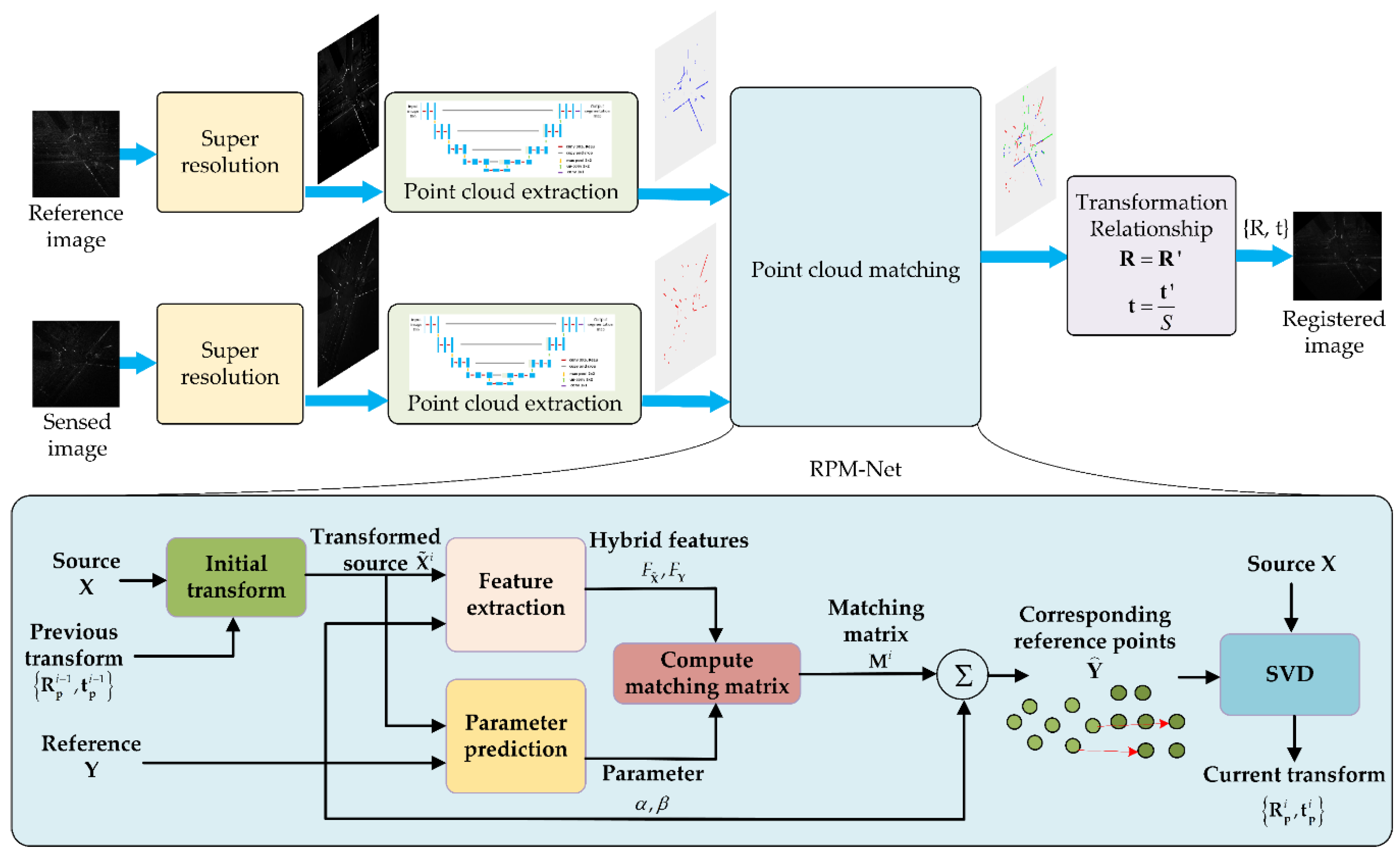
• A super-resolution structural point cloud matching framework for inter-frame registration of video-SAR is first proposed by integrating FRSR-Net, SPCE-Net with RPM-Net, which can significantly improve the registration accuracy and stableness of SAR images.
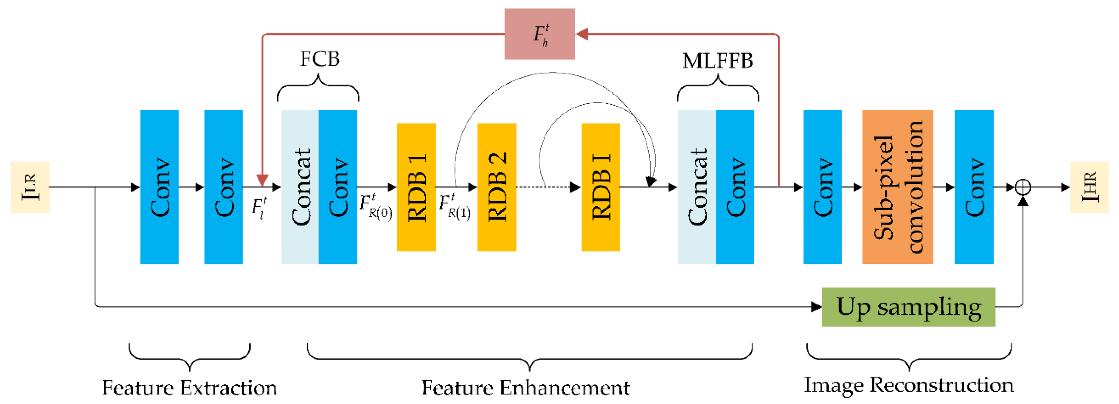
• A feature recurrent super-resolution network for video-SAR image super-resolution is proposed by refining the low-level features with the high-level features through feature recurrence, which is able to achieve elaborate image reconstruction.

The organization of the remaining sections of this paper is as follows. Section 2 reviews the principles of RPM-Net. The proposed S²-PCM framework is introduced in Section 3. Section 4 introduces the proposed FRSR-Net. Experimental results and analysis are given in Section 5. Finally, the conclusion is given in Section 6.

2. Review on Point Cloud Matching

As one of the most popular point cloud matching methods, the classical point cloud matching algorithms, including RPM and RPM-Net, are first reviewed in this section. RPM-Net [30] was proposed based on the RPM algorithm [31], which consists of two main modules: a feature extraction network and a parameter prediction network. It uses a differentiable Sinkhorn [32] layer and annealing [33] to obtain soft assignment values corresponding to points from hybrid features extracted from spatial coordinates and local geometry. To further improve the registration accuracy, a secondary network is added to predict the optimal annealing parameters.

Given the source point cloud X and the reference point cloud Y:

$$\begin{array}{c}X=\left\{x_j\in {ℝ}^3|j=1,\dots ,J\right\}\hfill \\ Y=\left\{y_k\in {ℝ}^3|k=1,\dots ,K\right\}\hfill \end{array}$$

(1)

where J and K are the numbers of points of X and Y, respectively, and J is not necessarily equal to K.

Point cloud registration is to find out the transformation relationship {R_p, t_p} between X and Y, where $R_p\in SO\left(3\right)$ is a rotation matrix and $t_p\in {ℝ}^3$ is a translation vector. To this end, a matching matrix $M\in {ℝ}^{J\times K}$ is defined to represent the correspondence between points, where each element m_jk can be determined by the following equation:

$$m_{jk}=\{\begin{array}{cc}1& \mathrm{if} \mathrm{point} x_j \mathrm{corresponds} \mathrm{to} y_k\\ 0& \mathrm{otherwise}\end{array}$$

(2)

The registration problem can be described as finding the {R_p, t_p} and the M that optimally maps points in X to Y, i.e.,

$$\underset{M,R_p,t_p}{\arg \min }{\displaystyle \sum _{j=1}^J{\displaystyle \sum _{k=1}^K{m}_{jk}}}\left({\Vert R_p{x}_j+t_p-y_k\Vert }_2^2-\alpha \right)$$

(3)

where ${\displaystyle {\sum }_{k=1}^K{m}_{jk}}=1,\forall j$, ${\displaystyle {\sum }_{j=1}^J{m}_{jk}}=1,\forall k$, and $m_{jk}\in \left\{0,1\right\}$. These three constraints require that M must be a permutation matrix. α is a parameter that controls the number of correspondences rejected as outliers.

In RPM, Equation (3) is minimized by two steps: soft assignment and transformation relationship estimation. Firstly, the constraint of the permutation matrix is relaxed to a double random matrix, i.e., $m_{jk}\in \left[0,1\right]$. Therefore, m_jk is initialized as:

$$m_{jk}\leftarrow e^{-\beta \left({\Vert R_p{x}_j+t_p-y_k\Vert }_2^2-\alpha \right)}$$

(4)

where β is an annealing parameter in each iteration. Then, the matching matrix M is estimated in the soft assignment. Once the optimal matching matrix is obtained, the transformation relationship can be computed.

In RPM-Net, the spatial distance in Equation (4) is replaced by the learned hybrid feature distance. In addition, α and β are obtained by network prediction. Specifically, RPM-Net solves the optimal transformation relationship by multiple iterations, as shown in Figure 1. In the ith iteration, the point cloud X is first transformed into the initial transformed point cloud ${\tilde{X}}^i$ by the transformation $\left\{R_p^{i-1},t_p^{i-1}\right\}$ estimated in the previous iteration. Then the feature extraction module extracts the hybrid features of ${\tilde{X}}^i$ and Y. Meanwhile, the optimal annealing parameters α and β are predicted by the secondary parameter prediction network. The initial matching matrix M is calculated using the hybrid features, and parameters α and β, i.e., m_jk is initialized as:

$$m_{jk}\leftarrow e^{-\beta \left({\Vert F_{{\tilde{x}}_j}-F_{y_k}\Vert }_2^2-\alpha \right)}$$

(5)

where $F_{{\tilde{x}}_j}$ and $F_{y_k}$ denote the hybrid features of points ${\tilde{x}}_j\in {\tilde{X}}^i$ and $y_k\in Y$ learned by the feature extraction network, respectively. Then the final matching matrix Mⁱ can be obtained by Sinkhorn normalization with enhanced double random constraints. Next, for each point x_j in X, its corresponding coordinate in Y is calculated as:

$${\widehat{y}}_j=\frac{1}{{\displaystyle {\sum }_k^K{m}_{jk}}}{\displaystyle \sum _k^K{m}_{jk}}●y_k$$

(6)

Finally, the transformation relationship is solved by SVD [34].

Since RPM-Net uses the learned feature distances instead of spatial distances to initialize the matching matrix, it avoids the initialization sensitivity and local minimum problems and is able to handle partial-to-partial point cloud registration. In addition, it improves the robustness to outliers by progressively reinforcing the soft assignment of point correspondences through Sinkhorn [32] and annealing [33], which is applied in this paper.

3. Super-Resolution Structural Point Cloud Matching Framework

Based on RPM-net, we present the framework of the super-resolution structural point cloud matching algorithm in detail in this section. In order to use the point clouds to register the SAR images, the point clouds first need to be extracted, which can be considered a segmentation problem in deep learning. Furthermore, to ensure the performance of the registration, the positions of the extracted point clouds should be accurate. However, for the actual SAR system, the images suffer from low resolution, speckle noise, blur and defocusing, which greatly reduce the image quality and lead to the difficulty and inaccuracy of the extraction of point clouds. Therefore, a novel super-resolution structural point cloud matching framework is presented in this section for better performance.

3.1. Network Structure

The proposed super-resolution structural point cloud matching (S²-PCM) framework for inter-frame registration of video-SAR consists of a super-resolution network, structural point cloud extraction network (SPCE-Net) and RPM-Net, as shown in Figure 1.

Firstly, the reference image I_ref and the sensed image I_sen are fed into a super-resolution network to improve the resolution and suppress the speckle noise. Most of the current super-resolution networks [35,36,37,38,39,40] are designed for optical images, but there are great differences between the textures of optical images and SAR images. Through experiments, it is found that the super-resolution network for optical images directly applying to SAR images results in poor performance. For this reason, we propose a super-resolution network, the details of which will be given in Section 4.

After image enhancement, feature point cloud extraction is required for SAR images. Extracting the point cloud can be achieved by fixing a threshold and selecting the points with higher intensity. It can also be achieved by segmentation. However, due to the different observation angles of the circular SAR system and the effect of speckle noise, the intensity of scattered points varies greatly among different images. The point clouds extracted by intensity-based methods vary greatly and reduce the registration accuracy significantly. Thus, we use the segmentation technique to extract the structural point clouds, i.e., point clouds reflecting the geometric structure of video-SAR frames. Firstly, we manually label the typical region edges in the video-SAR image to train a structural point cloud extraction network (SPCE-Net implemented by U-Net [41]). Secondly, the images are fed into the trained SPCE-Net to obtain the segmented masks. Then, the coordinates are extracted from the masks to generate the initial point clouds. To reduce the computational cost of the point cloud matching process, we down-sample the initial point clouds to generate the final structural point clouds via random sampling. Each structural point cloud contains approximately 1000 points. Too few points do not reflect the geometric structure of the image, which reduces the registration accuracy.

We use the trained SPCE-Net to segment the video-SAR frames to generate a sequence of point clouds, which is applied as the training dataset for RPM-Net. Then, we use the trained RPM-Net to match the structural point clouds. In order to achieve higher matching accuracy, RPM-Net requires at least five iterations. It is worth noting that since RPM-Net is a 3D point cloud registration network, we adapt the 2D point clouds extracted from the SAR images to RPM-Net by expanding a new dimension and setting it to 0. By feeding the structural point clouds into RPM-Net, we can obtain the transformation relationship {R′, t′} between images, where ${\mathbf{R}}^{\prime }\in SO\left(3\right)$ is a rotation matrix and ${\mathbf{t}}^{\prime }\in {ℝ}^3$ is a translation vector. Due to the scaling of super-resolution processing, the transformation relationship estimated by RPM-Net is not equal to the original one, which should be adjusted before use.

3.2. Transformation Relationship

Assume that the transformation relationship between I_sen and I_ref is {R, t}, where $R\in SO\left(3\right)$ is a rotation matrix and $t\in {ℝ}^3$ is a translation vector. According to [42], R, t can be expressed as:

$$\begin{array}{c}R=\left(\begin{array}{ccc}1& 0& 0\\ 0& \cos \varphi & \sin \varphi \\ 0& -\sin \varphi & \cos \varphi \end{array}\right)\left(\begin{array}{ccc}\cos \psi & 0& -\sin \psi \\ 0& 1& 0\\ \sin \psi & 0& \cos \psi \end{array}\right)\left(\begin{array}{ccc}\cos \theta & \sin \theta & 0\\ -\sin \theta & \cos \theta & 0\\ 0& 0& 1\end{array}\right)\hfill \\ t={\left(t_x,t_y,t_z\right)}^T\hfill \end{array}$$

(7)

where $\varphi$, $\psi$, and $\theta$ denote the rotation angles around the x-axis, y-axis, and z-axis, respectively, and t_x, t_y, and t_z denote the translations in the x-, y-, and z-directions, respectively. Since the sensed image I_sen and the reference image I_ref are located only in the x–y plane, it can be obtained that $\varphi$ and $\psi$ are 0 and t_z is 0. Equation (7) can be simplified as:

$$\begin{array}{c}R=\left(\begin{array}{ccc}\cos \theta & \sin \theta & 0\\ -\sin \theta & \cos \theta & 0\\ 0& 0& 1\end{array}\right)\hfill \\ t={\left(t_x,t_y,0\right)}^T\hfill \end{array}$$

(8)

Take any point A(x, y, 0) from I_sen and assume that its corresponding point in I_ref is B(x′, y′, 0), and then the relationship between A and B can be expressed as:

$$\left(\begin{array}{c}{x}^{\prime }\\ y^{\prime }\\ 0\end{array}\right)=R\left(\begin{array}{c}x\\ y\\ 0\end{array}\right)+t=\left(\begin{array}{ccc}\cos \theta & \sin \theta & 0\\ -\sin \theta & \cos \theta & 0\\ 0& 0& 1\end{array}\right)\left(\begin{array}{c}x\\ y\\ 0\end{array}\right)+\left(\begin{array}{c}{t}_x\\ t_y\\ 0\end{array}\right)$$

(9)

$$\cos \theta =\frac{O\overrightarrow{A}●O\overrightarrow{B}}{\left|O\overrightarrow{A}\right|\left|O\overrightarrow{B}\right|}$$

(10)

where O is the coordinate origin.

Given the scaling factor S of super-resolution, the points A(x, y, 0) and B(x′, y′, 0) after scale transformation are A′(Sx, Sy, 0) and B′(Sx′, Sy′, 0), respectively. Thus, the relationship between A′ and B′ can be expressed as:

$$\left(\begin{array}{c}{\mathit{Sx}}^{\prime }\\ {\mathit{Sy}}^{\prime }\\ 0\end{array}\right)={\mathbf{R}}^{\prime }\left(\begin{array}{c}Sx\\ Sy\\ 0\end{array}\right)+{\mathbf{t}}^{\prime }$$

(11)

Similar to Equation (10), we can obtain that the rotation angle around the z-axis of I_ref and I_sen after super-resolution is still θ. Thus, combining Equations (9) and (11), it can be obtained that:

$$\begin{array}{c}R={\mathbf{R}}^{\prime }\\ t=\frac{{\mathbf{t}}^{\prime }}{S}\end{array}$$

(12)

In a word, the transformation relationship {R′, t′} with a scaling operator between I_ref and I_sen is acquired by registration, and the transformation relationship {R, t} without a scaling operator between the original I_ref and I_sen can then be obtained according to Equation (12).

3.3. Training Strategy

Since it is hard to acquire noise-free high-resolution SAR images, we use optical images to construct the dataset for training a super-resolution network by data augmentation. Firstly, optical images are converted to grayscale images as high-resolution images for training. The high-resolution images are Bicubic [43] down-sampled and then blurred with a point spread function (PSF). Then, speckle noise of level L is added to construct low-resolution images. As a result, multiple pairs of training data are generated. We choose L1 loss for training the network, which is defined as:

$$L_{SR}={\displaystyle \sum _{y=1}^W{\displaystyle \sum _{x=1}^H\left|I_{SR}\left(x,y\right)-I_{HR}\left(x,y\right)\right|}}$$

(13)

where I_HR and I_SR denote the high-resolution image and the super-resolution image, respectively. W and H are the width and height of the image, respectively.

To train SPCE-Net, we label the images manually. Then the same affine transformation is applied to the images and the corresponding labels, thus achieving data augmentation and reducing the workload of image labeling. The dice coefficient [44] is used as the loss function for training SPCE-Net. It is an ensemble similarity measure function and calculated as follows:

$$Dice=\frac{2\left|T\cap P\right|}{\left|T\right|+\left|P\right|}$$

(14)

where T denotes the set of segmented true labels and P denotes the set of output predicted values. To calculate $\left|T\cap P\right|$, it is approximated as the sum of the dot product of T and P. $\left|T\right|+\left|P\right|$ denotes a direct summation over all elements of T and P. Thus, Diceloss can be obtained:

$$Diceloss=1-Dice$$

(15)

The overall loss L_seg uses the sum of Diceloss and the cross-entropy loss E:

$$L_{seg}=Diceloss+E$$

(16)

For training RPM-Net, we use the original point cloud as the source point cloud X. Then, we generate a random rotation angle around the z-axis in the range of [−90°, 90°] and a random translation vector in the range of [−300, 300] pixel on the x and y axes, which results in a transformation relationship {R_gt, t_gt}. This transformation relationship is applied to the source point cloud X to obtain the reference point cloud Y. For each point cloud, a hyperplane is randomly generated to sample a half-space, and it is continuously shifted so that 70% of the points are retained. Finally, Gaussian noise is added. We choose the L1 distance as the loss for training RPM-Net, which is defined as:

$$L_{reg}=\frac{1}{J}{\displaystyle \sum _j^J\left|\left(R_{gt}{x}_j+t_{gt}\right)-\left(R_{pred}{x}_j+t_{pred}\right)\right|}$$

(17)

where {R_pred, t_pred} is the prediction transformation.

4. Feature Recurrence Super-Resolution Network

In this section, we present our proposed feature recurrence super-resolution network in detail.

Most current super-resolution networks [35,36,37,38,39,40] for optical images reconstruct high-resolution images with only a single prediction, ignoring the connection between higher-level information and lower-level information. Since the resolution degradation of SAR images is affected by several factors, a single prediction may not be able to accurately recover the detailed information of the image. To this end, we design a feature recurrence super-resolution network (FRSR-Net) using the residual dense block (RDB) [40]. FRSR-Net utilizes a recurrence structure to refine low-level features with high-level features for better reconstruction of high-resolution SAR images, and the recurrence structure is able to reduce network parameters.

4.1. Super-Resolution Sub-Network via Feature Recurrence

The proposed FRSR-Net contains three modules: feature extraction, feature enhancement, and image reconstruction, as shown in Figure 2. The feature extraction module extracts the low-level features of the image. The feature enhancement module is mainly constructed by RDB, where RDB makes full use of the features of all convolutional layers within the block and establishes feature-to-feature associations with dense connections. Then, the local features generated by different RDBs are fused to generate high-level features. The image reconstruction module recovers high-resolution images by sub-pixel convolution [37].

The feature extraction module consists of two cascaded convolutional layers, and a ReLU activation function is connected after each convolutional layer. At the tth iteration, the low-level feature $F_l^t$, output by the feature extraction network, can be expressed as:

$$F_l^t=f_{FE}\left(I_{LR}\right)$$

(18)

where $f_{FE}(●)$ denotes the feature extraction module, and I_LR is the input of a low-resolution image.

The feature enhancement module consists of a feature compression block (FCB) cascaded with I RDBs, and a multi-level feature fusion block (MLFFB) is added last. At the tth iteration, the high-level feature $F_h^t$ is obtained by feeding the low-level feature $F_l^t$ and the hidden feature $F_h^{t-1}$ output from the feature enhancement module in the previous iteration into the feature enhancement module, which can be expressed by the following equation:

$$F_h^t=f_{EN}\left(F_l^t,F_h^{t-1}\right)$$

(19)

where $f_{EN}(●)$ denotes the feature enhancement module. At the initial iteration, $F_h^{t-1}$ is initialized to $F_l^t$. Specifically, $F_l^t$ is concatenated with $F_h^{t-1}$ as the input to FCB to obtain the feature $F_{R\left(0\right)}^t$ as the input to RDB 1. Then, the output of the previous RDB is used as the input to the next RDB, i.e.,

$$\begin{array}{c}{F}_{R\left(0\right)}^t=f_{FCB}\left(F_l^t,F_h^{t-1}\right)\hfill \\ F_{R\left(i\right)}^t=f_{RDB,i}\left(F_{R\left(i-1\right)}^t\right)=f_{RDB,i}\left(f_{RDB,i-1}\left(\dots \left(f_{RDB,1}\left(F_{R\left(0\right)}^t\right)\right)\dots \right)\right)\hfill \end{array}$$

(20)

where $f_{FCB}(●)$ denotes FCB, $f_{RDB,i}(●)$ denotes the ith RDB, and $F_{R\left(i\right)}^t$ denotes the local features of the output of the ith RDB. Finally, the MLFFB connects all the local features and applies a convolution operation to obtain the high-level feature $F_h^t$, i.e.,

$$F_h^t=f_{MLFFB}\left(F_{R\left(1\right)}^t,F_{R\left(2\right)}^t,\dots ,F_{R\left(I\right)}^t\right)$$

(21)

where $f_{MLFFB}(●)$ denotes MLFFB.

The image reconstruction module consists of two convolutional layers and a sub-pixel convolution block [37], and more details of sub-pixel convolution will be introduced in Section 4.3. $F_h^t$ is used as the input of the first convolution layer, and then the feature map is up-sampled by a subpixel convolution block. Finally, I_LR is bilinearly interpolated and added to the output of the image reconstruction module to obtain the reconstruction output I_SR, i.e.,

$$I_{SR}^t=f_{IR}\left(F_h^t\right)+f_{up}\left(I_{LR}\right)$$

(22)

where $f_{IR}(●)$ denotes the image reconstruction module and $f_{up}(●)$ denotes the bilinear up-sampling.

After T_a rounds of iterations, the output of the T_ath iteration is taken as the final reconstructed image.

4.2. Residual Dense Block

Since the details of SAR images are obscured by the strong speckle noise, the standard convolutional networks that are composed of simple chain stacking may ignore some information about each convolutional layer. On the contrary, thee RDB proposed by Zhang et al. [40] uses dense connection and residual connection, which fully utilizes the information of the convolutional layer within the block and has the stable characteristic to extract the detailed information of SAR images. RDB mainly contains dense connection layers, local feature fusion and local residual learning, as shown in Figure 3.

There are N_c convolutional layers within each RDB, and each convolutional layer except for the last layer is followed by a ReLU. The dense connection is reflected in the interconnection between the convolutional layers, i.e., the input of the nth convolutional layer in RDB is the output of the previous (n − 1) convolutional layers connected to the input of RDB. Therefore, the output $F_{R\left(i,n\right)}$ of the nth convolutional layer of the ith RDB can be expressed as:

$$F_{R\left(i,n\right)}=\sigma \left(W_{i,n}\left[F_{R\left(i-1\right)},F_{R\left(i,1\right)},\dots ,F_{R\left(i,n-1\right)}\right]+b_{i,n}\right)$$

(23)

where σ denotes the linear activation unit, and W_i,n and b_i,n denote the weight and bias of the nth convolutional layer within the ith RDB, respectively.

Then, local feature fusion is performed. The output of all convolutional layers within the current ith RDB and the input of RDB are connected into a 1 × 1 convolutional block, and the output is obtained as the feature $F_{LF\left(i\right)}$:

$$F_{LF\left(i\right)}=f_{conv,i}\left(\left[F_{R\left(i-1\right)},F_{R\left(i,1\right)},F_{R\left(i,2\right)},\dots ,F_{R\left(i,N_c\right)}\right]\right)$$

(24)

where $f_{conv,i}(●)$ denotes the last convolution operation of the ith RDB. In this way, the local features of the previous RDB flow into the next RDB by direct concatenation, which can greatly reduce the number of features and achieve the full utilization of features.

Finally, local residual learning is utilized to better improve the information flow. The local feature $F_{R\left(i\right)}$ of the output of the ith RDB can be expressed as:

$$F_{R\left(i\right)}=F_{R\left(i-1\right)}+F_{LF\left(i\right)}$$

(25)

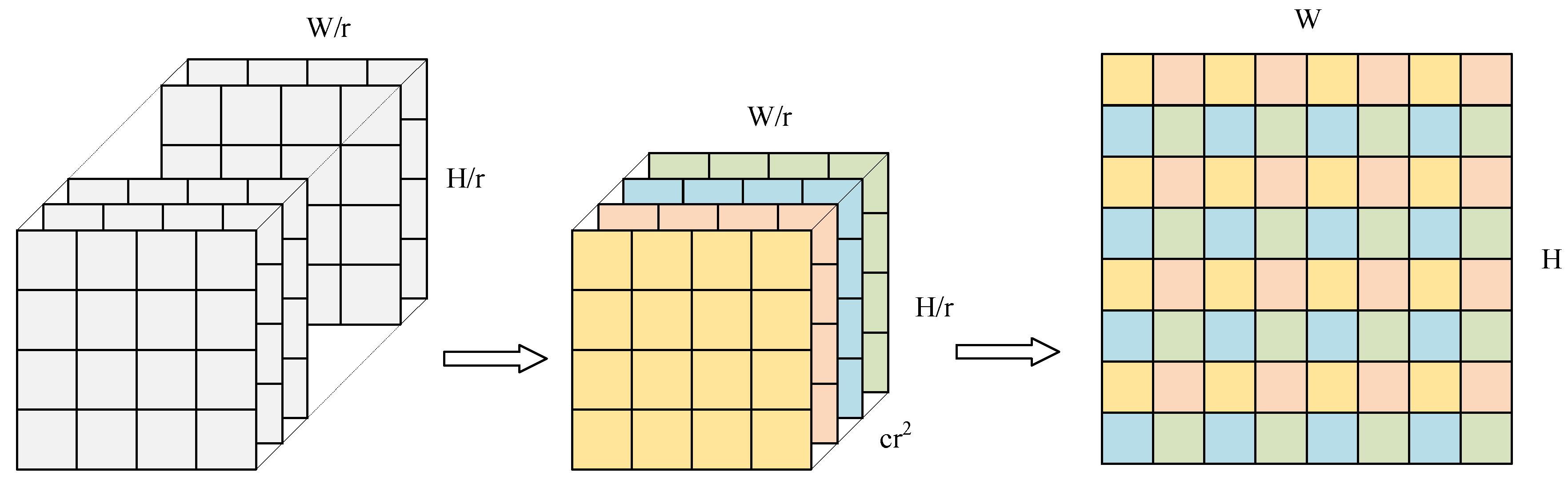
4.3. Sub-Pixel Convolution

In super-resolution tasks, the commonly used image up-sampling methods are interpolation, deconvolution, and sub-pixel convolution [37]. The parameters of interpolation-based up-sampling methods are not obtainable by learning, while the deconvolution tends to introduce a checkerboard effect to the image. In order to ensure the trainability of the reconstruction parameters and achieve efficient up-sampling, sub-pixel convolution is applied here.

Sub-pixel convolution, also called pixel shuffling, exploits a channel-to-space conversion method to achieve spatial magnification by rearranging the pixels in multiple channels of the feature map, as shown in Figure 4. Suppose we need to up-sample the feature map $F_{in}\in {ℝ}^{W/r\times H/r\times c{r}^2}$ by a factor of r, where $W/r$, $H/r$, and $c{r}^2$ denote the width, height, and the number of channels of the feature map, respectively. Sub-pixel convolution is used to obtain the output:

$$F_{out}\left(x,y,c\right)=F_{in}\left(\lfloor x/r\rfloor ,\lfloor y/r\rfloor ,c\times r\times \mathrm{mod}\left(y,r\right)+c\times \mathrm{mod}\left(x,r\right)+c\right)$$

(26)

where $F_{out}\left(x,y,c\right)$ is the value at position (x, y) on the cth channel of the output, $\mathrm{mod}(●)$ denotes the remainder operation, and $\lfloor ●\rfloor$ represents the function to find the maximum integer that does not exceed the given input. For example, a feature map of size 32 × 32 × 4 is up-sampled twice, the number of feature channels is reduced after pixel shuffling, and the elements are rearranged to obtain an output of 64 × 64 × 1.

5. Experiments and Results

5.1. Dataset and Setting

DIV2K [40] is a common dataset for super-resolution tasks in optics, containing a total of 1000 high-resolution images, of which 800 were used for training, 100 for validation and 100 for testing. Therefore, according to the strategy in Section 3.3, we used 800 training images from DIV2K to construct the dataset for training FRSR-Net and used five validation images during the training process. In the down-sampling, scaling factors of two, three, and four were applied, respectively. For testing, we selected several standard test datasets for the super-resolution task, including Set14 [40], Manga109 [40], and some images from the test set of DIV2K. Among them, set14 contains 14 optical images and Manga109 consists of 109 manga, which are commonly used as test datasets in super-resolution tasks. The test datasets were prepared by the same processing steps as the training dataset.

For training SPCE-Net and RPM-Net, we selected a simulated video-SAR dataset and a real video-SAR dataset. The real video-SAR dataset contains 500 images, and the simulated video-SAR data contains 500 images. The networks were trained with these two datasets separately.

To test the registration performance of our S²-PCM, we selected three test datasets containing a video-SAR simulation dataset and two video-SAR real datasets. Each test dataset contains 50 continuous frames. In the later subsection, we refer to the two real datasets as real dataset 1 and real dataset 2, respectively.

In the super-resolution experiment, the number of iterations was set to 4, and the number of RDBs was 8 in FRSR-Net. In the registration experiments, the scaling factor of super-resolution was set to 3, and the registration of each dataset was taken by registering the later images to the initial frame. The whole experiment was implemented with the Pytorch open-source framework and trained with the Intel i7-8700 CPU and NVIDIA GTX-1080 (8G) GPU hardware platform.

5.2. Evaluation Metrics

5.2.1. Super-Resolution Evaluation Metrics

We used the widely used peak signal-to-noise ratio (PSNR) [45] and structural similarity (SSIM) [46] to evaluate the super-resolution performance. PSNR is defined as follows:

$$PSNR=10{\log }_{10}\left(\frac{MA{X}_I^2}{MSD}\right)$$

(27)

where MAX_I is the maximum pixel value in the image, and MSD is the mean squared difference between the two images.

SSIM is a metric that measures the degree of similarity between images. It is more consistent with the human eye’s judgment of image quality compared with PSNR, which is defined as follows:

$$SSIM=\frac{\left(2{\mu }_x{\mu }_y+C_1\right)\left(2{\sigma }_{xy}+C_2\right)}{\left({\mu }_x^2+{\mu }_y^2+C_1\right)\left({\sigma }_x^2+{\sigma }_y^2+C_2\right)}$$

(28)

where μ_x, μ_y are the means of x and y, σ_x and σ_y are the standard deviations of x and y, σ_xy is the covariance of x and y, and C₁ and C₂ are constants.

5.2.2. Registration Evaluation Metrics

In order to quantitatively evaluate the registration performance of S²-PCM, the following evaluation metrics [47,48] were applied. Firstly, we used the symbols M and N to denote the random variables of the statistical features of the reference image and the registered image, respectively.

• Pearson correlation coefficient (PCC):

$$PCC=\frac{1}{l-1}{\displaystyle \sum _{i=1}^l\left(\frac{m_i-{\mu }_M}{{\sigma }_M}\right)}\left(\frac{n_i-{\mu }_N}{{\sigma }_N}\right)$$

(29)

where m_i and n_i denote the realizations of the random variables M and N, l is the length of the random variable, µ_M, µ_N are the means of M and N, and σ_M and σ_N are the standard deviations of M, N.

2.

Mean squared differences (MSD):

$$MSD=\frac{1}{l}{\displaystyle \sum _{i=1}^l{\left(m_i-n_i\right)}^2}$$

(30)

where m_i, n_i, and l are the same as in Equation (29).

3.

Mutual information (MI):

$$MI=I\left(M,N\right)={\displaystyle \sum _{m\in M}{\displaystyle \sum _{n\in N}{p}_{M,N}}}\left(m,n\right)\log \frac{p_{M,N}\left(m,n\right)}{p_M\left(m\right)p_N\left(n\right)}$$

(31)

where $p_M\left(m\right)$ and $p_N\left(n\right)$ denote the one-dimensional probability densities of the normalized histograms of M and N, respectively. $p_{M,N}\left(m,n\right)$ denotes the two-dimensional joint probability densities of the normalized joint histograms of M and N.

4.

Normalized mutual information (NMI):

$$\begin{array}{cc}\hfill NMI=& \frac{H\left(M\right)+H\left(N\right)}{H\left(M,N\right)}\hfill \\ \hfill H\left(M,N\right)=& -{\displaystyle \sum p_{M,N}}\left(m,n\right)\log \left(p_{M,N}\left(m,n\right)\right)\hfill \\ \hfill H\left(M\right)=& -{\displaystyle \sum p_M}\left(m\right)\log \left(p_M\left(m\right)\right)\hfill \\ \hfill H\left(N\right)=& -{\displaystyle \sum p_N}\left(n\right)\log \left(p_N\left(n\right)\right)\hfill \end{array}$$

(32)

where $p_M\left(m\right)$, $p_N\left(n\right)$, and $p_{M,N}\left(m,n\right)$ are the same as in the above equation, H(M) and H(N) are the entropies of M and N, respectively, and H(M, N) is the joint entropy of the pair (M, N).

5.

Entropy correlation coefficient (ECC):

$$ECC=\sqrt{\frac{2I\left(M,N\right)}{H\left(M\right)+H\left(N\right)}}$$

(33)

where I(M, N), H(M), and H(N) are given by the above equation.

6.

SSIM is given in Section 5.2.1.

Among the above evaluation metrics, MI, NMI, and ECC are information theory-based evaluation methods, and MSD, PCC, and SSIM are statistical-based evaluation methods.

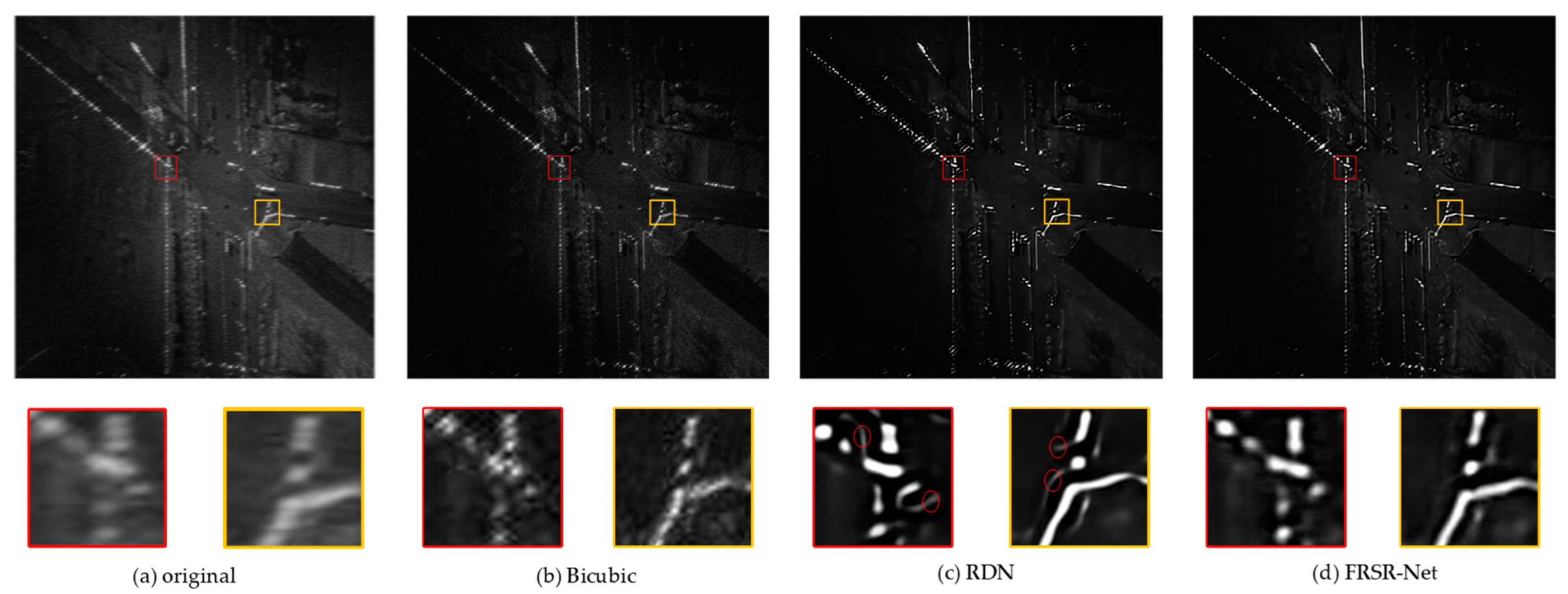
5.3. Analysis of Super-Resolution Performance

In this sub-section, we verify and analyze the super-resolution performance of FRSR-Net. We compare FRSR-Net with two other super-resolution methods. One is the traditional Bicubic algorithm [43], and the other is the deep learning-based RDN [40]. We train RDN with the same dataset.

Firstly, we verify the super-resolution performance with three test datasets, and the experimental results of super-resolution with different scaling factors are shown in

Table 1. Average PSNR/SSIM values.

Dataset	Scaling Factor	Bicubic	RDN	FRSR-Net
Set14	2	16.8536/0.1850	23.1123/0.5920	23.3392/0.6015
	3	16.3669/0.1696	21.5473/0.5301	21.7953/0.5406
	4	16.0525/0.1734	20.4009/0.4907	20.6160/0.4986
Manga109	2	15.2934/0.1592	21.8103/0.7003	22.3246/0.7189
	3	14.7603/0.1473	20.0737/0.6393	20.3832/0.6554
	4	14.4211/0.1583	18.9417/0.6042	19.1847/0.6156
DIV2K	2	17.3878/0.1789	25.2677/0.6623	25.5155/0.6679
	3	17.0843/0.1766	23.9786/0.6190	24.1894/0.6245
	4	16.9035/0.1918	23.0580/0.5954	23.2885/0.6007

. It can be seen from Table 1 that all the evaluation metrics of FRSR-Net are superior to the rest of the compared methods, and it achieves the best performance. The test results of RDN are the second, and Bicubic is the worst.

FRSR-Net takes full advantage of the features of different levels of RDB and adopts a recurrence structure to refine the low-level features with the high-level output features, which results in better reconstruction performance. Since Bicubic is not able to learn the mapping from low-resolution images to high-resolution images, it has the worst test results. Due to the use of the recurrence structure, FRSR-Net applies a smaller number of RDBs compared with RDN, which results in a smaller number of parameters for the network. With a super-resolution scaling factor of three, the number of network parameters of FRSR-Net is about 1.7 million, and that of RDN is about 3.6 million. It can be seen that the number of parameters used in our method is less than 50% of that of RDN.

The calculation of the above metrics requires noise-free high-resolution images as reference, but it is not possible to obtain real SAR images without the influence of noise. In order to verify the super-resolution performance of our method on real SAR images, a real SAR image is applied to super-resolution with a scaling factor of three. We qualitatively compare the super-resolution results of the FRSR-Net with the above comparison methods, as shown in Figure 5.

It can be seen from Figure 5 that, compared with the remaining two methods, our method achieves the best visual effect. Specifically, some details of the image are recovered in the results, the edges of the image are sharpened, and the speckle noise is suppressed. Compared with the original image, the RDN recovered image detail is not accurate enough, and it generates some additional textures, as shown by the red circles in the enlarged subfigure. The super-resolution effect of Bicubic is the worst, which only enlarges the image and cannot recover image details and suppress speckle noise.

5.4. Analysis of Registration Performance

In this sub-section, we verify the registration performance of our S²-PCM on a simulated dataset and real dataset, respectively. We compare our S²-PCM with three traditional algorithms, including SIFT, SAR-SIFT and PSO-SIFT [49]. We match the feature points using the nearest neighbor distance ratio (NNDR) with Euclidean distance and eliminate all incorrectly matched feature points using the Fast Sample Consensus (FSC) algorithm [50], which divides the candidate objects in Random Sample Consensus (RANSAC) [51] into two parts: the sample set with a high correct rate and the consensus set with large correct matches. Compared with RANSAC, FSC can achieve a greater number of correct feature point matching with fewer iterations.

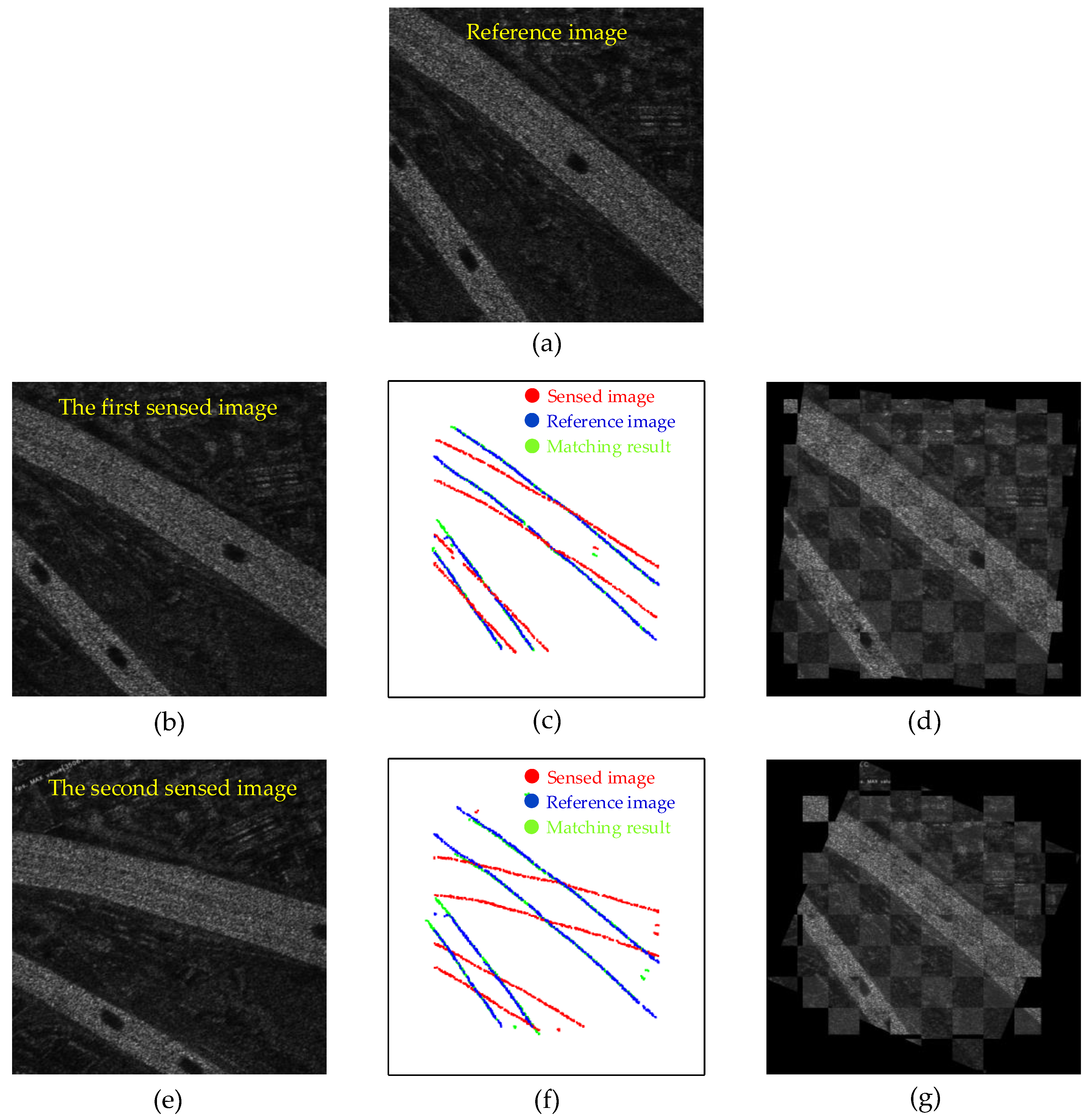
5.4.1. Registration Results of Simulation Dataset

The registration results of the simulated dataset are shown in

Table 2. Comparison of SIFT, SAR-SIFT, PSO-SIFT and the proposed method on the simulated dataset.

	MI	NMI	ECC	MSD	PCC	SSIM
SIFT	4.0214	1.5011	0.8167	758.6585	0.5180	0.2684
SAR-SIFT	4.2285	1.5053	0.8192	622.5073	0.5566	0.2867
PSO-SIFT	4.2582	1.5031	0.8179	616.7051	0.5426	0.2929
Proposed	4.2764	1.5058	0.8196	551.6772	0.5921	0.2702

. It can be seen that the proposed S²-PCM method is superior to the compared methods with most of the metrics. However, due to the simplicity of the simulated scenes, the registration performance of SAR-SIFT and PSO-SIFT is acceptable with most image pairs, and the proposed method has only a slight superiority over them. Since the moving targets’ shadows in the simulated SAR images are vivid and similar, we find that the three comparison methods regard the moving targets’ shadows as feature descriptors. Since the moving targets’ shadows are always moving, there are some error conversion relationships, which lead to the degradation of the registration performance.

As shown in Figure 6, we select two representative images to show the registration results of our S²-PCM. Figure 6c,f shows the matching results of the structural point clouds, where the red points denote the structural point clouds of the sensed images, the blue points are the structural point clouds of the reference image, and the green points are the point clouds after being matched. The green point cloud is completely overlapped with the blue point cloud and has a good registration result. Figure 6d,g is the checkerboard mosaicked images [24] after registration, and the brightness of the images is adjusted. The edge continuity between the registered image and the reference image can be seen in the figure, which indicates the excellent registration performance of our method.

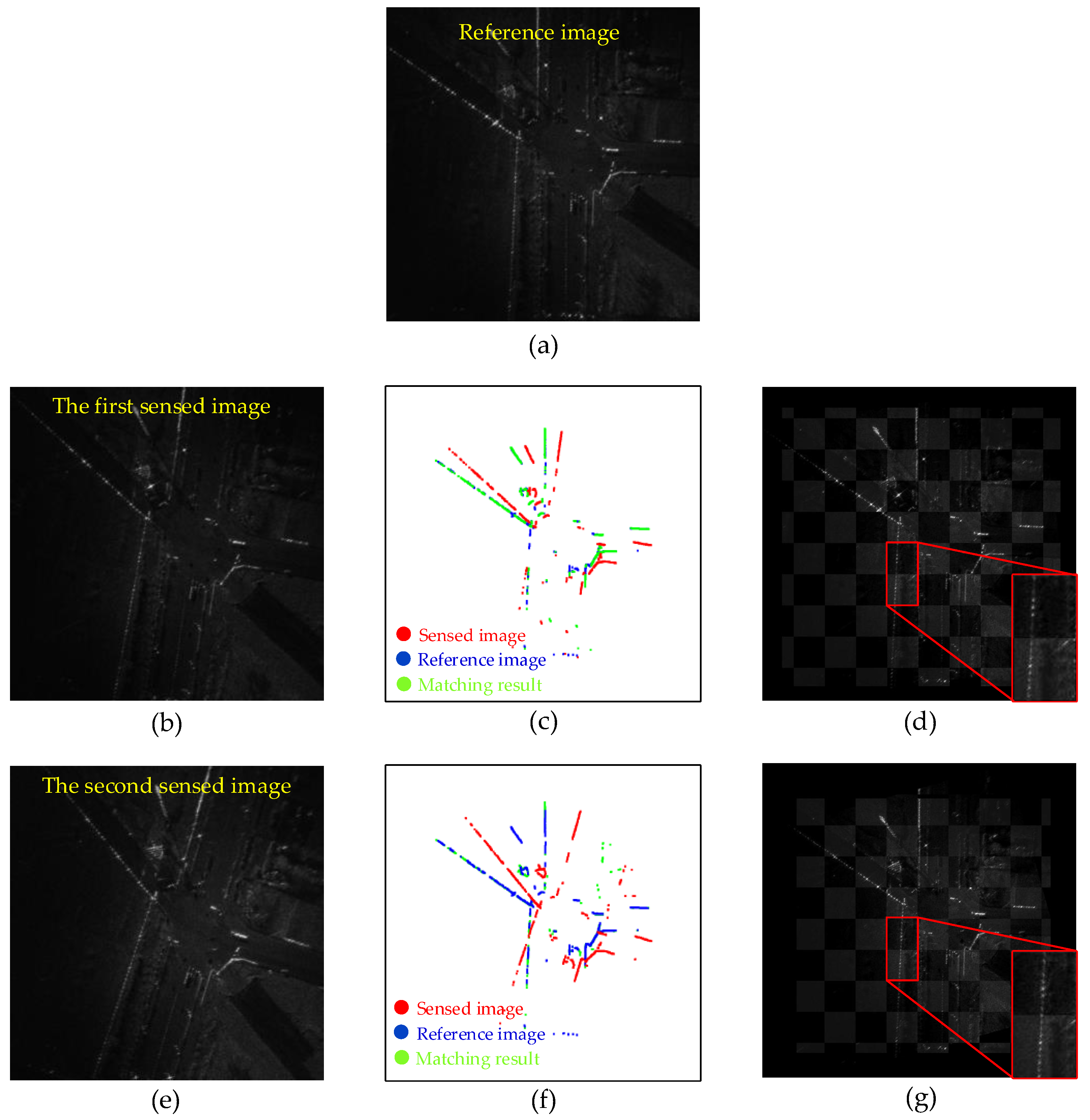
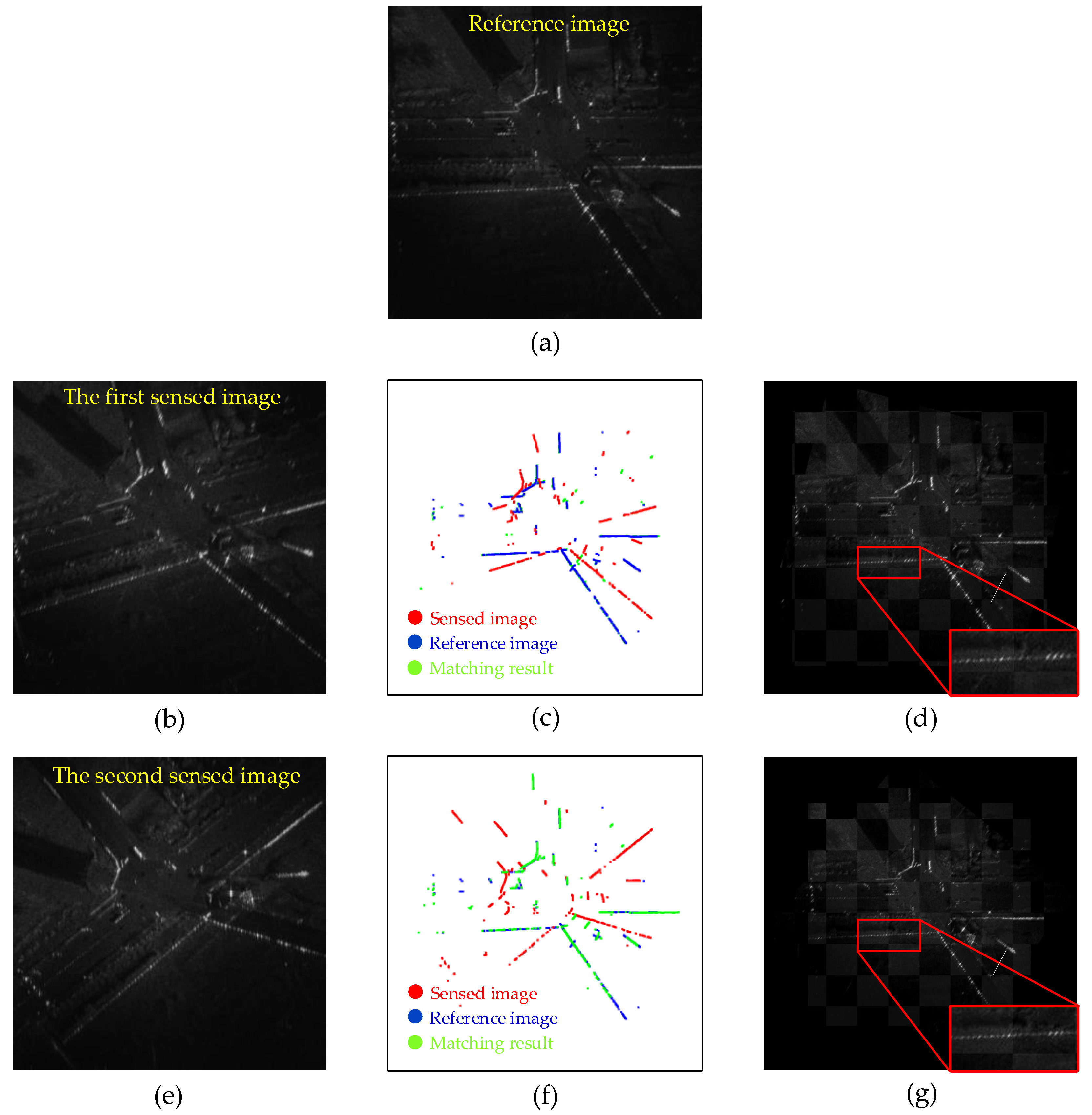
5.4.2. Registration Results of Real Datasets

In the two real test datasets, the images’ quality of real dataset 1 is better than that of real dataset 2, and some images of real dataset 2 appear defocused. Both have large speckle noise and brightness variation between images. A comparison of the registration results is shown in

Table 3. Comparison of SIFT, SAR-SIFT, PSO-SIFT and proposed method on real dataset 1.

	MI	NMI	ECC	MSD	PCC	SSIM
SIFT	3.6440	1.5976	0.8639	136.6799	0.6462	0.6936
SAR-SIFT	3.7013	1.6105	0.8698	118.1341	0.7014	0.7229
PSO-SIFT	3.7276	1.6138	0.8714	119.7662	0.7135	0.7269
Proposed	3.8130	1.6271	0.8777	102.6517	0.7458	0.7544

and

Table 4. Comparison of SIFT, SAR-SIFT, PSO-SIFT and proposed method on real dataset 2.

	MI	NMI	ECC	MSD	PCC	SSIM
SIFT	3.5571	1.5852	0.8572	187.7355	0.6203	0.6051
SAR-SIFT	3.7284	1.6057	0.8674	147.3779	0.7181	0.6564
PSO-SIFT	3.7644	1.5979	0.8640	149.6696	0.6639	0.6667
Proposed	3.8850	1.6217	0.8753	111.4737	0.7586	0.7083

. We can observe from the tables that the registration performance of our method is superior to other comparison methods on both datasets under MI, NMI, ECC, MSD, PCC, and SSIM evaluation metrics. Moreover, the registration performance on dataset 2 is significantly better than the comparison methods, which indicates that the S²-PCM method is relatively robust to image defocusing. In summary, our method uses structural point clouds, which reflect the geometric characteristics of images, as matching features. Due to the enhancement of image details and suppression of speckle noise by super-resolution, the structural point clouds are extracted more accurately, which is beneficial for improving registration accuracy. In addition, the RPM-Net, which is robust to outliers and desensitized to initialization, is used to match the point clouds, which further improves registration accuracy.

As mentioned in reference [20,21], the calculation of the dominant direction of the SIFT algorithm is strongly influenced by speckle noise, which will affect the matching performance of the feature descriptors. During experiments, we find that due to the texture characteristic of the SAR image, there are sometimes only a few correctly matched feature point pairs (less than four feature point pairs) persevered by the SIFT-like algorithms after the FSC algorithm. In this case, the registration fails.

To demonstrate the registration performance of our S²-PCM more intuitively, for each dataset, we select two representative sensed images and draw the registration results, as shown in Figure 7 and Figure 8, where Figure 7 shows the results of real dataset 1 and Figure 8 shows the results of real dataset 2. The matching results of the point clouds are shown in Figure 7c,f and Figure 8c,f. It can be seen that the green point cloud has almost been overlapped with the blue point cloud, which shows a good matching performance. Figure 7d,g and Figure 8d,g are the checkerboard mosaicked images after registration, and we zoom in for the details in the image. From the figures, we can see that the edges of the image after registration and the reference image are continuous, and the regions are overlapped well, which indicates that our S²-PCM method is able to achieve excellent registration performance.

5.5. Ablation Study

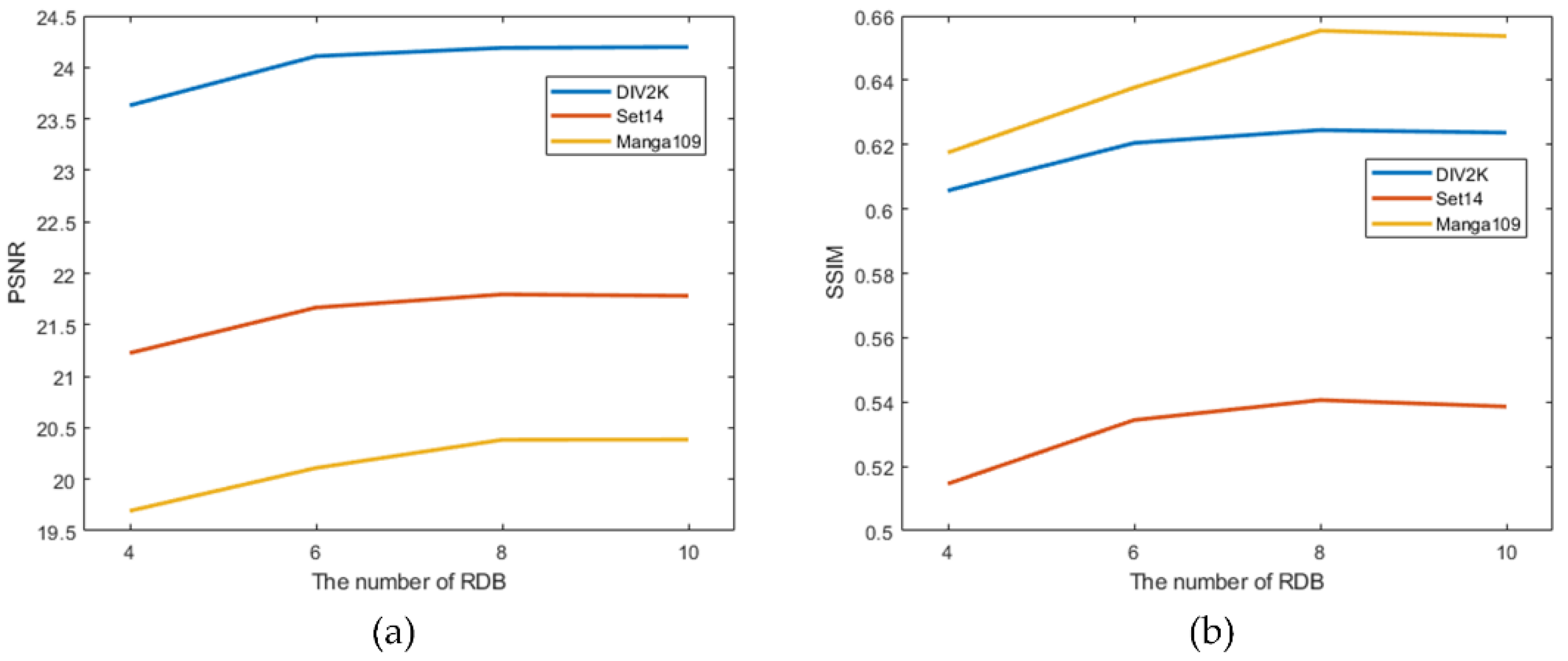
5.5.1. Super-Resolution Performance with Different Numbers of RDBs

In this sub-section, we analyze the effect of different numbers of RDBs on the super-resolution performance of FRSR-Net. With a super-resolution scaling factor of three, we perform experiments on three super-resolution test datasets, and Figure 9 shows the experimental results.

It can be seen from Figure 9 that the PSNR and SSIM metrics increase as the number of RDBs increases, which suggests that increasing the number of RDBs is beneficial to improving the super-resolution performance of the network. The main reason is that more RDBs indicates a deeper network with stronger feature extraction capacity. When the number of RDBs is greater than eight, we find that PSNR and SSIM increase slightly or even stop at a certain point. However, as the number of RDBs increases, the network is more complex and time-consuming. Therefore, we believe that when the number of RDBs is eight, there is a good balance between network performance and complexity.

5.5.2. Super-Resolution Registration Results with Different Scaling Factors

In this subsection, the effects of different super-resolution scaling factors on the registration performance are discussed. We reselect 30 real video-SAR images to compare the registration performance with different super-resolution scaling factors, and the results are shown in

Table 5. Comparison of the registration with different super-resolution scaling factors.

Scaling Factor	MI	NMI	ECC	MSD	PCC	SSIM
1	4.1025	1.6166	0.8734	134.2960	0.7652	0.7007
2	4.1840	1.6401	0.8834	98.3499	0.8570	0.7504
3	4.1887	1.6413	0.8839	95.8823	0.8611	0.7530
4	4.1779	1.6384	0.8827	101.3225	0.8480	0.7471

. From the table, it can be seen that the registration performance of video-SAR images after super-resolution is significantly better than that without super-resolution, indicating that the use of super-resolution is beneficial in improving the registration accuracy of images. This is mainly because the FRSR-Net highlights the edge features of the image and suppresses the speckle noise, which makes the extraction of the structural point cloud easier and more accurate. The best registration performance is achieved when the scaling factor of the super-resolution is three. A possible reason is that as the scaling factor increases, the performance of the super-resolution network becomes unstable.

6. Conclusions

In this paper, the super-resolution structural point cloud matching (S2-PCM) framework is proposed for video-SAR inter-frame registration, which consists of FRSR-Net, SPCE-Net and RPM-Net. The main conclusions are as follows:

• Compared with the classical SIFT-like algorithms, S²-PCM has higher registration accuracy for video-SAR images under diverse evaluation metrics, such as MI, NMI, ECC, SSIM, etc.
• By integrating feature recurrence structure and RDB, the proposed FRSR-Net can significantly improve the quality of video-SAR images and point cloud extraction accuracy. Combining FRSR-Net with S²-PCM, we can obtain higher registration accuracy.
• Increasing the number of RDBs is beneficial in improving the super-resolution performance of FRSR-Net. Experimental results show that when the number of RDBs is eight, an excellent balance between network complexity and performance is achieved.
• The scaling factor has a significant effect on the results, and a reasonable super-resolution scale should be chosen. Too high a super-resolution scaling factor may lead to the unstable performance of FRSR-Net. Experimental results show that the highest registration accuracy can be obtained when the scaling factor is three.

Our future work will focus on two aspects. The first is to deal with the linear deformation in video-SAR images, which might lead to the RPM-Net failure. Furthermore, we will take on more endeavors on the problem of multi-source point cloud extraction and image registration.

References

1. Song, X.; Yu, W. Processing video-SAR data with the fast backprojection method. IEEE Trans. Aerosp. Electron. Syst. 2016, 52, 2838–2848. [Google Scholar] [CrossRef]
2. Yang, X.; Shi, J.; Zhou, Y.; Wang, C.; Hu, Y.; Zhang, X.; Wei, S. Ground moving target tracking and refocusing using shadow in video-SAR. Remote Sens. 2020, 12, 3083. [Google Scholar] [CrossRef]
3. Jun, S.; Long, M.; Xiaoling, Z. Streaming BP for non-linear motion compensation SAR imaging based on GPU. IEEE J. Sel. Top. Appl. Earth Obs. Remote Sens. 2013, 6, 2035–2050. [Google Scholar] [CrossRef]
4. Chen, F.; Lasaponara, R.; Masini, N. An overview of satellite synthetic aperture radar remote sensing in archaeology: From site detection to monitoring. J. Cult. Herit. 2017, 23, 5–11. [Google Scholar] [CrossRef]
5. Zhou, Y.; Shi, J.; Wang, C.; Hu, Y.; Zhou, Z.; Yang, X.; Wei, S. SAR Ground Moving Target Refocusing by Combining mRe³ Network and TVβ-LSTM. IEEE Trans. Geosci. Remote Sens. 2020, 60, 1–14. [Google Scholar]
6. Yang, X.; Shi, J.; Chen, T.; Hu, Y.; Zhou, Y.; Zhang, X.; Wu, J. Fast Multi-Shadow Tracking for Video-SAR Using Triplet Attention Mechanism. IEEE Trans. Geosci. Remote Sens. 2022, 60, 1–12. [Google Scholar] [CrossRef]
7. Ding, J.; Wen, L.; Zhong, C.; Loffeld, O. Video SAR moving target indication using deep neural network. IEEE Trans. Geosci. Remote Sens. 2020, 58, 7194–7204. [Google Scholar] [CrossRef]
8. Rui, J.; Wang, C.; Zhang, H.; Jin, F. Multi-Sensor SAR Image Registration Based on Object Shape. Remote Sens. 2016, 8, 923. [Google Scholar] [CrossRef]
9. Cui, S.; Xu, M.; Ma, A.; Zhong, Y. Modality-free feature detector and descriptor for multimodal remote sensing image registration. Remote Sens. 2020, 12, 2937. [Google Scholar] [CrossRef]
10. Fan, J.; Wu, Y.; Wang, F.; Zhang, P.; Li, M. New point matching algorithm using sparse representation of image patch feature for SAR image registration. IEEE Trans. Geosci. Remote Sens. 2016, 55, 1498–1510. [Google Scholar] [CrossRef]
11. Xing, C.; Qiu, P. Intensity-based image registration by nonparametric local smoothing. IEEE Trans. Pattern Anal. Mach. Intell. 2011, 33, 2081–2092. [Google Scholar] [CrossRef]
12. Sarvaiya, J.N.; Patnaik, S.; Bombaywala, S. Image Registration by Template Matching Using Normalized Cross-Correlation. In Proceedings of the 2009 International Conference on Advances in Computing, Control, and Telecommunication Technologies, Bangalore, India, 28–29 December 2009; pp. 819–822. [Google Scholar]
13. Mahmood, A.; Khan, S. Correlation-coefficient-based fast template matching through partial elimination. IEEE Trans. Image process. 2011, 21, 2099–2108. [Google Scholar] [CrossRef]
14. Kern, J.P.; Pattichis, M.S. Robust multispectral image registration using mutual-information models. IEEE Trans. Geosci. Remote Sens. 2007, 45, 1494–1505. [Google Scholar] [CrossRef]
15. Suri, S.; Reinartz, P. Mutual-information-based registration of TerraSAR-X and Ikonos imagery in urban areas. IEEE Trans. Geosci. Remote Sens. 2009, 48, 939–949. [Google Scholar] [CrossRef]
16. Thévenaz, P.; Unser, M. Optimization of mutual information for multiresolution image registration. IEEE Trans. Image Process. 2000, 9, 2083–2099. [Google Scholar] [PubMed]
17. Lowe, D. Distinctive image features from scale-invariant keypoints. Int. J. Comput. Vis. 2004, 20, 91–110. [Google Scholar] [CrossRef]
18. Ke, Y.; Sukthankar, R.; Society, I.C. PCA-SIFT: A More Distinctive Representation for Local Image Descriptors. In Proceedings of the 2004 IEEE Computer Society Conference on Computer Vision and Pattern Recognition (CVPR 2004), Washington, DC, USA, 27 June–2 July 2004; pp. 506–513. [Google Scholar]
19. Dellinger, F.; Delon, J.; Gousseau, Y.; Michel, J.; Tupin, F. Sar-sift: A sift-like algorithm for sar images. IEEE Trans. Geosci. Remote Sens. 2013, 53, 453–466. [Google Scholar] [CrossRef]
20. Xiang, Y.; Wang, F.; Wan, L.; You, H. An Advanced Rotation Invariant Descriptor for SAR Image Registration. Remote Sens. 2017, 9, 686. [Google Scholar] [CrossRef]
21. Fan, B.; Wu, F.; Hu, Z. Aggregating gradient distributions into intensity orders: A novel local image descriptor. In Proceedings of the 2011 IEEE Conference on Computer Vision and Pattern Recognition (CVPR), Colorado Springs, CO, USA, 20–25 June 2011; pp. 2377–2384. [Google Scholar]
22. Wang, S.; Quan, D.; Liang, X.; Ning, M.; Guo, Y.; Jiao, L. A deep learning framework for remote sensing image registration. ISPRS J. Photogramm. Remote Sens. 2018, 145, 148–164. [Google Scholar] [CrossRef]
23. Han, X.; Leung, T.; Jia, Y.; Sukthankar, R.; Berg, A.C. Matchnet: Unifying feature and metric learning for patch-based matching. In Proceedings of the IEEE Conference on Computer Vision and Pattern Recognition, Boston, MA, USA, 7–12 June 2015; pp. 3279–3286. [Google Scholar]
24. Mao, S.; Yang, J.; Gou, S.; Jiao, L.; Xiong, T.; Xiong, L. Multi-Scale Fused SAR Image Registration Based on Deep Forest. Remote Sens. 2021, 13, 2227. [Google Scholar] [CrossRef]
25. Besl, P.J.; McKay, N.D. Method for registration of 3-D shapes. In Sensor Fusion IV: Control Paradigms and Data Structures; SPIE: Bellingham, WA, USA, 1992; pp. 586–606. [Google Scholar]
26. Yang, J.; Li, H.; Campbell, D.; Jia, Y. Go-ICP: A globally optimal solution to 3D ICP point-set registration. IEEE Trans. Pattern Anal. Mach. Intell. 2015, 38, 2241–2254. [Google Scholar] [CrossRef] [Green Version]
27. Wang, Y.; Solomon, J.M. Deep closest point: Learning representations for point cloud registration. In Proceedings of the IEEE/CVF International Conference on Computer Vision, Seoul, Korea, 27 October–2 November 2019; pp. 3523–3532. [Google Scholar]
28. Aoki, Y.; Goforth, H.; Srivatsan, R.A.; Lucey, S. Pointnetlk: Robust & efficient point cloud registration using pointnet. In Proceedings of the IEEE/CVF Conference on Computer Vision and Pattern Recognition; 2019; pp. 7163–7172. [Google Scholar]
29. Sarode, V.; Li, X.; Goforth, H.; Aoki, Y.; Srivatsan, R.A.; Lucey, S.; Choset, H. Pcrnet: Point cloud registration network using pointnet encoding. arXiv 2019, arXiv:1908.07906. [Google Scholar]
30. Yew, Z.J.; Lee, G.H. Rpm-net: Robust point matching using learned features. In Proceedings of the IEEE/CVF Conference on Computer Vision and Pattern Recognition, Seattle, WA, USA, 14–19 June 2020; pp. 11824–11833. [Google Scholar]
31. Gold, S.; Rangarajan, A.; Lu, C.P.; Pappu, S.; Mjolsness, E. New algorithms for 2D and 3D point matching: Pose estimation and correspondence. Pattern Recognit. 1998, 31, 1019–1031. [Google Scholar] [CrossRef]
32. Sinkhorn, R. A relationship between arbitrary positive matrices and doubly stochastic matrices. Ann. Math. Stat. 1964, 35, 876–879. [Google Scholar] [CrossRef]
33. Kirkpatrick, S.; Gelatt, C.D., Jr.; Vecchi, M.P. Optimization by simulated annealing. Science 1983, 220, 671–680. [Google Scholar] [CrossRef]
34. Papadopoulo, T.; Lourakis, M.I. Estimating the jacobian of the singular value decomposition: Theory and applications. In European Conference on Computer Vision; Springer: Berlin, Heidelberg, 2000; pp. 554–570. [Google Scholar]
35. Dong, C.; Loy, C.C.; He, K.; Tang, X. Image super-resolution using deep convolutional networks. IEEE Trans. Pattern Anal. Mach. Intell. 2015, 38, 295–307. [Google Scholar] [CrossRef]
36. Dong, C.; Loy, C.C.; Tang, X. Accelerating the super-resolution convolutional neural network. In Lecture Notes in Computer Science, Proceedings of the European Conference on Computer Vision, Amsterdam, The Netherlands, 11–14 October 2016; Springer: Cham, Switzerland, 2016; pp. 391–407. [Google Scholar]
37. Shi, W.; Caballero, J.; Huszár, F.; Totz, J.; Aitken, A.P.; Bishop, R.; Rueckert, D.; Wang, Z. Real-time single image and video super-resolution using an efficient sub-pixel convolutional neural network. In Proceedings of the IEEE Conference on Computer Vision and Pattern Recognition, Las Vegas, NV, USA, 26 June–1 July 2016; pp. 1874–1883. [Google Scholar]
38. Kim, J.; Lee, J.K.; Lee, K.M. Accurate image super-resolution using very deep convolutional networks. In Proceedings of the IEEE Conference on Computer Vision and Pattern Recognition, Las Vegas, NV, USA, 26 June–1 July 2016; pp. 1646–1654. [Google Scholar]
39. Lim, B.; Son, S.; Kim, H.; Nah, S.; Mu Lee, K. Enhanced deep residual networks for single image super-resolution. In Proceedings of the IEEE Conference on Computer Vision and Pattern Recognition Workshops, Honolulu, HI, USA, 21–26 June 2017; pp. 136–144. [Google Scholar]
40. Zhang, Y.; Tian, Y.; Kong, Y.; Zhong, B.; Fu, Y. Residual dense network for image super-resolution. In Proceedings of the IEEE Conference on Computer Vision and Pattern Recognition, Salt Lake City, UT, USA, 18–22 June 2018; pp. 2472–2481. [Google Scholar]
41. Ronneberger, O.; Fischer, P.; Brox, T. U-net: Convolutional networks for biomedical image segmentation. In International Conference on Medical Image Computing and Computer-Assisted Intervention; Springer: Cham, Switzerland, 2015; pp. 234–241. [Google Scholar]
42. Slabaugh, G.G. Computing Euler angles from a rotation matrix. Retrieved August 1999, 6, 39–63. [Google Scholar]
43. De Boor, C. Bicubic spline interpolation. J. Math. Phys. 1962, 41, 212–218. [Google Scholar] [CrossRef]
44. Shamir, R.R.; Duchin, Y.; Kim, J.; Sapiro, G.; Harel, N. Continuous dice coefficient: A method for evaluating probabilistic segmentations. arXiv 2019, arXiv:1906.11031. [Google Scholar]
45. Goodman, J.W. Statistical properties of laser speckle patterns. In Laser Speckle and Related Phenomena; Springer: Berlin/Heidelberg, Germany, 1975; pp. 9–75. [Google Scholar]
46. Wang, Z.; Bovik, A.C.; Sheikh, H.R.; Simoncelli, E.P. Image quality assessment: From error visibility to structural similarity. IEEE Trans. Image Process. 2004, 13, 600–612. [Google Scholar] [CrossRef]
47. Penney, G.P.; Weese, J.; Little, J.A.; Desmedt, P.; Hill, D.L. A comparison of similarity measures for use in 2-D-3-D medical image registration. IEEE Trans. Med. Imaging 1998, 17, 586–595. [Google Scholar] [CrossRef] [PubMed]
48. Razlighi, Q.R.; Kehtarnavaz, N.; Yousefi, S. Evaluating similarity measures for brain image registration. J. Vis. Commun. Image Represent. 2013, 24, 977–987. [Google Scholar] [CrossRef] [PubMed]
49. Ma, W.; Wen, Z.; Wu, Y.; Jiao, L.; Gong, M.; Zheng, Y. Remote sensing image registration with modified sift and enhanced feature matching. IEEE Geosci. Remote Sens. Lett. 2016, 14, 3–7. [Google Scholar] [CrossRef]
50. Wu, Y.; Ma, W.; Gong, M.; Su, L.; Jiao, L. A novel point-matching algorithm based on fast sample consensus for image registration. IEEE Geosci. Remote Sens. Lett. 2015, 12, 43–47. [Google Scholar] [CrossRef]
51. Fischler, M.A.; Bolles, R.C. Random sample consensus: A paradigm for model fitting with applications to image analysis and automated cartography. Commun. ACM 1981, 24, 381–395. [Google Scholar] [CrossRef]
Figure 1. Super-resolution structural point cloud matching (S2-PCM) framework.
Remotesensing 14 04302 g001
Figure 2. The architecture of the feature recurrence super-resolution network (FRSR-Net).
Remotesensing 14 04302 g002
Figure 3. The architecture of residual dense block (RDB).
Remotesensing 14 04302 g003
Figure 4. The sub-pixel convolutional operation.
Remotesensing 14 04302 g004
Figure 5. Visual results of super-resolution.
Remotesensing 14 04302 g005
Figure 6. Registration results on simulated dataset. (a) Reference image. (b) The first sensed image. (c) Point cloud matching result of the first sensed image. (d) Checkerboard mosaicked image of the first sensed image. (e) The second sensed image. (f) Point cloud matching result of the second sensed image. (g) Checkerboard mosaicked image of the second sensed image.
Remotesensing 14 04302 g006
Figure 7. Registration results on real dataset 1. (a) Reference image. (b) The first sensed image. (c) Point cloud matching result of the first sensed image. (d) Checkerboard mosaicked image of the first sensed image. (e) The second sensed image. (f) Point cloud matching result of the second sensed image. (g) Checkerboard mosaicked image of the second sensed image.
Remotesensing 14 04302 g007
Figure 8. Registration results on real dataset 2. (a) Reference image. (b) The first sensed image. (c) Point cloud matching result of the first sensed image. (d) Checkerboard mosaicked image of the first sensed image. (e) The second sensed image. (f) Point cloud matching result of the second sensed image. (g) Checkerboard mosaicked image of the second sensed image.
Remotesensing 14 04302 g008
Figure 9. Test results for different numbers of RDBs. (a) PSNR metric. (b) SSIM metric.
Remotesensing 14 04302 g009