Abstract
Exposed mine gangue hills are prone to environmental problems such as soil erosion, surface water pollution, and dust. Revegetation of gangue hills can effectively combat the problem. Effective ground cover monitoring means can significantly improve the efficiency of vegetation restoration. We used UAV aerial photography to acquire data and used the Real-SR network to reconstruct the data in super-resolution; the Labv3+ network was used to segment the ground cover into green areas, open spaces, roads, and waters, and VDVI and Otsu were used to extract the vegetation from the green areas. The final ground-cover decomposition accuracy of this method can reach 82%. The application of a super-resolution reconstruction network improves the efficiency of UAV aerial photography; the ground interpretation method of deep learning combined with a vegetation index solves both the problem that vegetation index segmentation cannot cope with the complex ground and the problem of low accuracy due to little data for deep-learning image segmentation.
1. Introduction
1.1. Gangue Hill for the Necessity of Vegetation Restoration
A large number of coal mines in China are concentrated in the provinces of Shanxi, Inner Mongolia, Shaanxi and Ningxia. There are 11 large coal mining bases in arid and semi-arid regions, such as the north and northwest of China. These areas are already ecologically fragile, desertification is severe, and a large amount of coal mining has made the ecological environment of the grassland areas even more unstable, which, in turn, has affected the development of local livestock. Drainage sites and gangue hills are typical types of damage formed during the coal-mining process in the arid desert areas of northwest China, mainly consisting of coal gangue, rocks, and soil. The soil structure of the drainage field is loose, with low nutrient content and more developed macro porosity. Its soil’s physical and chemical properties and the ecological environment differ significantly from the natural landscape. At the same time, the crushing of automated vehicles during the soil piling process leads to severe compaction of the ground surface, which is not conducive to the rooting and growth of vegetation. Under constant high-temperature exposure, the dark-colored land also tends to absorb a large amount of solar energy, and the surface is rich in coal debris, posing serious fire-safety hazards; under rainfall and windy conditions, the exposed soil discharge site is prone to environmental problems such as soil erosion, surface water pollution and dust, which have a terrible impact on the surrounding ecological environment and people’s lives. Necessary vegetation restoration is beneficial to improve the ecological environment near the mine, reduce soil erosion and desertification, improve slope stability of gangue hills, and increase sunlight reflectivity. The study area selected for this paper is located in the Luotua Mountain and Mengxi mining areas in Wuhai, Inner Mongolia. It is a typical northwest open pit mine, and its research results have a tremendous role in monitoring vegetation restoration in northwest coal mines.
1.2. Difficulties of Vegetation Greening
Although revegetation of the area around the open pit is a pressing issue, due to the low precipitation in the semi-arid region, natural revegetation has low coverage and long lead times, requiring manual intervention. However, the lack of water makes revegetation costly. Effective revegetation monitoring can reduce maintenance costs by replacing periodic full irrigation sprinklers with timely manual intervention in poorly restored areas. At the same time, more accurate ground interpretation allows for better comparison of restored areas with bare areas and timely monitoring of the dynamics of water storage lakes and roads.
Remote-sensing means are used for vegetation identification mainly by extracting remote sensing image information for interpretation. Traditional remote-sensing monitoring methods are mostly satellite remote sensing, which uses images of different spatial, spectral, and temporal resolutions for regional monitoring and analysis. However, for the specific application scenario of monitoring vegetation recovery in mining areas, satellite remote sensing has several disadvantages as follows:
- Due to the limitation of image resolution, the accuracy of thematic information extracted through satellite remote-sensing images has a particular gap with the actual value. For the drainage field, a typical disturbed patch in the mining area, its scope is relatively small, and the identification of vegetation species and the quantitative monitoring study of soil erosion cannot be well achieved by traditional remote-sensing monitoring.
- High-resolution satellite data is expensive. According to the internationally accepted calculation method, on average, the development, launch, and insurance cost of an artificial satellite is nearly 1.4 billion RMB, which does not include the post-processing and transmission of the satellite remote-sensing images of ground receiving station costs and labor costs. So, the cost of remote sensing images is high, especially if the gangue mountain used for landforms changes within a short period. The images are required to have higher definition and complete feature information.
With the mature development of UAV technology in the past two years, UAVs, as a new means of remote sensing, have unique advantages compared to traditional satellite remote sensing and manned aerial remote sensing:
- Relatively inexpensive drones with low operating and maintenance costs;
- UAV flight has low site requirements. It can adopt a variety of take-off and landing methods without the need for professional take-off and landing runways, and can operate in mountainous areas, gullies, rivers, and other areas. It cannot be reached by human power;
- UAVs are relatively simple to operate, easy to maintain, and can deal with temporary on-site problems positively and effectively.
However, during field operations, the aircraft flies at a higher altitude from the ground due to factors affecting flight safety, such as undulating terrain and easily blocked signal propagation, resulting in lower ground resolution. We need to introduce image super-resolution techniques into the pre-processing of UAV images.
1.3. Related Work
H. Shen proposed a super-resolution image reconstruction algorithm to moderate-resolution imaging spectroradiometer (MODIS) remote-sensing images. In the registration part, a truncated quadratic cost function is used to exclude the outlier pixels, which strongly deviate from the registration model [1].
X. Qifang used an interpolation reconstruction method to reconstruct satellite video images, so that the reconstructed static features have smoother and clearer edges and richer detail information, which can effectively improve the resolution of satellite video images [2]. In the multi-frame remote-sensing image Super-Resolution (SR) reconstruction based on Back-Propagation (BP) neural network, Ding et al. used a three-layer BP neural network to perform super-resolution reconstruction of the input remote-sensing images. The amount of computation performed by the BP neural network is also particularly outstanding due to a large amount of data it requires to converge. Although genetic algorithms can find globally optimal solutions and are highly robust, the algorithm is not sufficiently convergent [3]. Chen and Wang combined the genetic algorithm with the BP neural network to give the network faster convergence and more vital learning ability [4]. Ma et al. proposed a transient Generative-Adversarial-Networks (GAN)-based method for SR reconstruction of remote sensing images, which improved the previous SR-GAN [5]. Specifically, by removing components, the traditional GAN is simplified to reduce memory requirements and improve computational performance. In addition, inspired by migration learning, their reconstruction method was pre-trained on the DIV2K dataset and then tuned using the remotely sensed image dataset, leading to higher accuracy and visual performance. Johanna’s study investigated the physically-based characterization of mixed floodplain vegetation by means of terrestrial laser scanning (TLS). The work aimed at developing an approach for deriving the characteristic reference areas of herbaceous and foliated, woody vegetation, and estimating the vertical distribution of woody vegetation [6]. ZM’s review provided few outlooks in understanding the underlying od the ML models application for HM simulation [7]. Mohammad proposed a three-dimensional hole size (3DHS) analysis for separating extreme and low-intensity events observed during experimental runs [8]. Lama’s study aimed at quantifying analytically the uncertainty in flow average velocity estimations associated with the uncertainty of Leaf Area Index (LAI) of Phragmites australis (Cav.) Trin. ex Steudel covering a vegetated channel [9]. Shen’s review paper was intended to provide water resources scientists and hydrologists, in particular, with a simple technical overview, transdisciplinary progress update, and a source of inspiration about the relevance of DL to water [10,11]. The Vegetation Index (VI) method is the most common, economical, and effective method for extracting and analyzing vegetation information over a large area using remote sensing data. It is based on using different wavelengths in images from satellites in orbit (most commonly the visible red, green, and blue wavelengths and the near-infrared wavelengths) in different mathematical combinations for vegetation studies. There are currently more than 100 vegetation indices proposed in remote sensing. However, most of them are based on the visible-NIR bands, such as the more common normalized difference vegetation index (NDVI) [12], the ratio vegetation index (RVI), and the NIR band.
The leading vegetation indices are EXG (excess green) [13], NGRDI (normalized green-red difference index) [14], and EVI (enhanced vegetation index) [12]. There are few vegetation indices based only on visible wavelengths. It mainly includes EXG (excess green), NGRDI (normalized green-red difference index), NGBDI (normalized green-blue difference index) [15], and RGRI (red-green ratio index) modeled based on the NGRDI structure.
In recent years, scholars have also increasingly applied deep-learning models to remote-sensing images to obtain better recognition results. Natesan et al. [16] applied the residual network (Resnet) to RGB images, which contained different tree types, and used the trained model for classification, achieving 80% classification accuracy; Yang et al. [17]. took the high spatial resolution remote sensing images World View-2 from Bazhou City, Hebei Province, as the data source and selected the deep convolutional SegNet, a deep convolutional neural network, to extract rural buildings from remote-sensing images. Lobo et al. [18]. used five deep, fully convolutional networks: SegNet, U-Net, FCN-DenseNet, and two DeepLabv3+ network variants to semantically classify single tree species in UAV visible images of urban areas. In segmentation, the performance of the five models was evaluated in terms of classification accuracy and computational effort. The experimental analysis showed that the average overall accuracy of the five methods ranged from 88.9% to 96.7%. The experiments also showed that the addition of a Conditional Random Field (CRF) could improve the performance of the models but required higher computational effort; Ren et al. [19]. applied deep learning to the detection of rural buildings in UAV remote-sensing imagery and used the Faster R-CNN network model to identify rural buildings quickly and accurately. The overall accuracy of this method exceeded 90%. Zhou et al. [20] compared the traditional segmentation model with the semantic segmentation method DeepLabv3+ to segment the remote sensing images acquired by UAV under different environments with leaf coverage images, and the results showed that the DeepLabv3+ model could obtain better segmentation results. Long et al. [21] first used a well-known classification network (VGG16) for end-to-end semantic segmentation, being completely convolutional, and upsampling the output feature mapping. However, the direct use of these networks leads to rough pixel output caused by multiple upsampling in order to collect more context information in the classification task. To output more precisely, Long proposed to use jump connections to fuse deep and shallow network features. Morales et al. [22] used three RGB cameras to obtain aerial images of palm trees under different environmental and lighting conditions. They trained the DeeplabV3+ network for areas that are difficult to investigate in the field, such as swamps. The test set on the model achieved an accuracy of 98.14% and was able to identify not only free-standing palm trees but also palm trees partially covered by other types of vegetation, which is highly practical.
The main advantages of our method are: (1) The introduction of super-resolution algorithms into the processing of remote sensing images, which improves the spatial resolution of images without affecting the interpretation. (2) Suitable visible vegetation indices and thresholds were selected for the northwest’s specific topographical and geomorphological features, and the accurate extraction of vegetation was achieved. (3) A dataset for the interpretation of specific mining areas based on aerial images from UAVs was produced, and a deep-learning network was used for ground interpretation to improve vegetation monitoring in mining areas and reduce the cost of vegetation restoration.
2. Materials and Experimental Design
2.1. Study Area
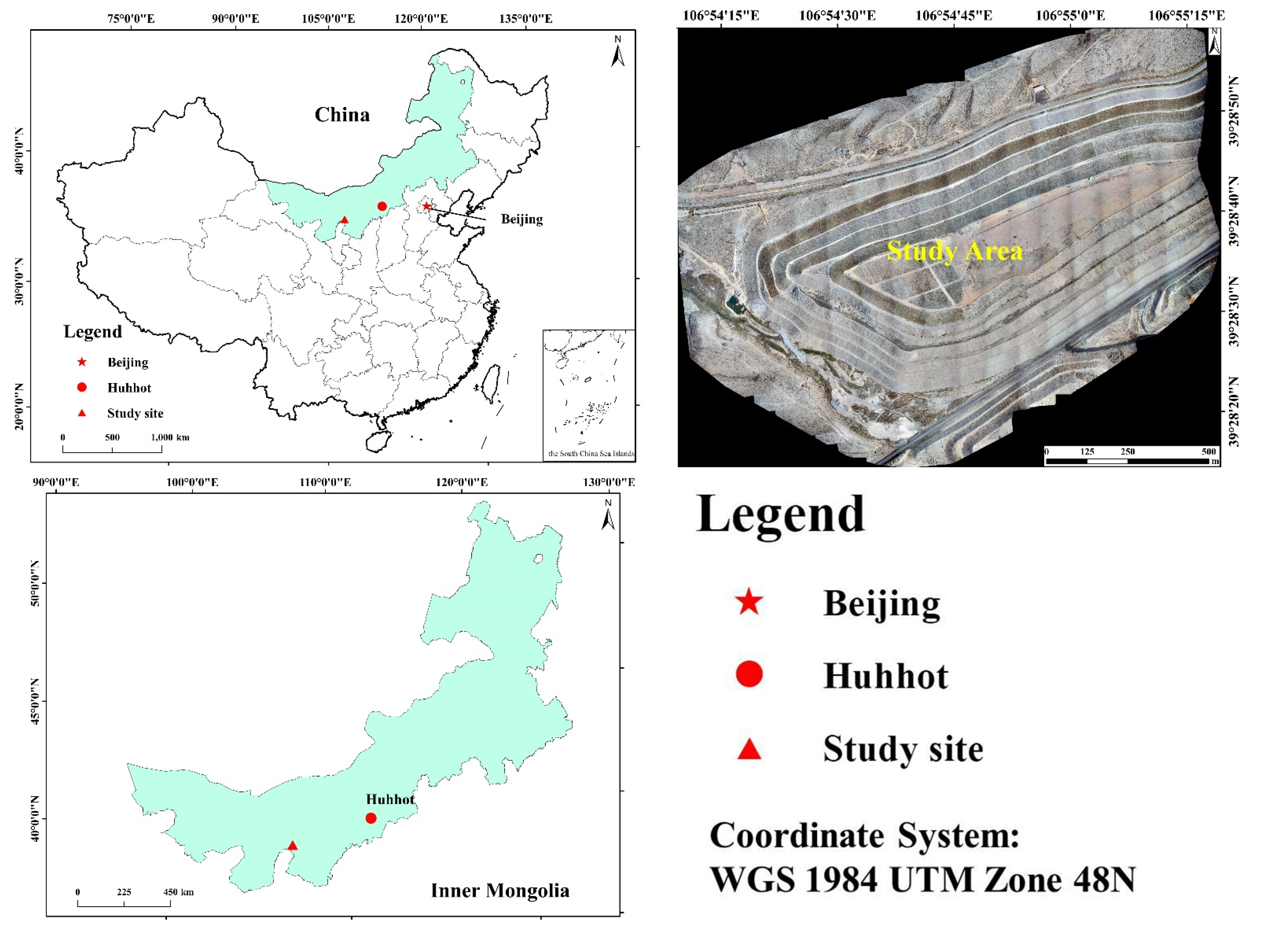
Our study site is in two typical mining gangue hills in Wuhai, Inner Mongolia, China. The climate in the study area is arid, and precipitation is scarce, with an average annual temperature of 9.2 °C, average annual precipitation of 162 mm, and a multi-year average annual evaporation of 3286 mm, nearly 20 times the average annual precipitation. The vegetation in the study area is mainly artificially established herbaceous plants, including Medicagosativa, Bassia dasyphyllous, Suaedaglauca, Astragalus surgeons, Setaria viridis, Agriophyllum, and Astragalus, Agriophyllum squarrose, etc., with low average cover and fragile ecosystems. Figure 1 displays the study area.
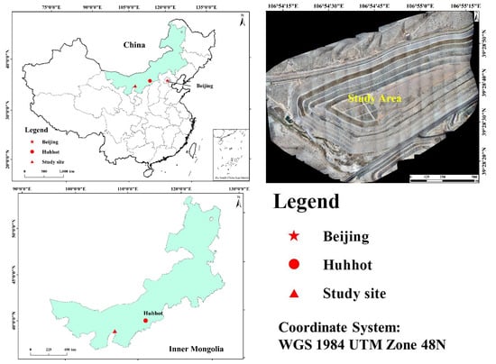
Figure 1.
Study Area.
2.2. Data Acquisition
We used aerial images from May, June, and July 2022 (UAV parameters) UAV model was Pegasus D2000, flight speed was 13.5 m/s, heading overlap rate was 80%, side overlap rate was 60%, operating line height was 384 m. The sensor size was 23.5 × 15.6 mm, the lens was 25 mm fixed focal length, and the effective pixels were about 24.3 million. The GSD was calculated to be 6cm. In order to produce a resolution reconstruction network control group, one operation was carried out at 192 m height in the Camelot mine with a GSD of 3 cm.
We stitched the flight data taken by the UAV at 192 m altitude and cropped a total of 1350 images of 1500 × 1000 size for training, using the dataset of 384 m flight for Super-resolution reconstruction experiments. The flight data for both altitudes in this section had the same time scale and were in the same study area.
In the subsequent application of the algorithm, the trained super-resolution reconstruction model will be used to reconstruct the images taken at the height of 384 m. Ground deciphering and segmentation used the reconstructed images.
2.3. Experimental Design for Classification
To enhance the ground resolution of the images, we used real-sr networks [23] for super-resolution reconstruction of the images. We compared them with ESRGAN [24], WAIFU2X [25], and SRMD [26] methods at a 2-fold increase in image resolution.
The original UAV images were stitched by lens correction, cropped, and processed into 512 × 384 images. The ground conditions were divided into four types (vegetation recovery areas, bare ground, roads, and water) for image segmentation and annotation in labeling I to prepare a deep learning dataset for remote-sensing interpretation. The Deep Labv3+ network with the Mask-R-CNN network was used for training and testing. The classification scheme was set up as a two-stage classification system, where the stitched and cropped images reconstructed at resolution were placed in the classifier. The first level used deep-learning segmentation to define four types of ground interpretation: vegetation restoration areas, bare land, roads, and water. The second level used the visible vegetation index method to define vegetation restoration areas and bare land as vegetation areas, non-vegetation areas, respectively.
The overall vegetation cover, as well as the respective vegetation cover of the revegetated areas and bare ground, was calculated from the image count.
3. Methods
3.1. Deeplab V3+
We employed a neural network structure integrating feature fusion and atrous convolution to segment the grass images with low vegetation coverage and address the issue of grass segmentation under the circumstances of low vegetation coverage. By shooting offline, we first constructed the image data. The data was then split into a training set and a test set after the original data had been processed to produce the image form corresponding to each image for semantic segmentation. The network structure was then modified based on DeepLabv3+. We changed the feature extraction network in the backbone to MobilenetV2, and we changed the output channels’ number to 3, which stands for the three objects that are most common in green spaces: vegetation, roads, and water sources. The grass segmentation model was then created using the prepared grass data for training. In order to get segmentation results, the test set was lastly tested using the grass segmentation model. This section is structured as follows: Section 3.1.1 presents the Atrous convolution method, Section 3.1.2 briefly covers the Mobilenetv2 backbone feature-extraction network, and Section 3.1.3 provides a detailed description of the structure of our model.
3.1.1. Atrous Convolution
The grass in the picture resembles typical land before it was entirely developed and the drones frequently maintained a relatively high flight height when conducting shooting operations in search of a larger shooting area. The two factors mentioned above will interfere with grass identification. That is to say, because grassland images were so particular, we must consider the interference that traditional land caused while identifying grassland. To solve this issue, we wanted our convolution to have a larger perceptual field to gather more data from the image. This would lead to better results in practice, as we gathered more detailed data through a larger perceptual field and improve the performance of our grass recognition model when performing grass recognition.
Moreover, downsampling and larger convolutional kernels were two more conventional methods for enlarging the perceptual field. In the first scenario, downsampling frequently causes an image’s resolution to drop, obliterating some fine details and impairing our model’s ability to recognize the grass. As a result, this was a bad strategy for our grass detection model. In the second instance, increasing the convolutional kernel did broaden the perceptual field, as shown in Figure 2. However, depending on the size of the convolutional kernel, a feature point was replaced in the upper feature layer with a different number of feature points, meaning that the amount of information captured also varies. Naturally, a bigger convolutional kernel would have a more significant perceptual field, gathering more data and making it easier for us to distinguish the grass from other similar regions. However, a larger convolutional kernel also had drawbacks because it entailed more parameters, increasing program runtime. As a result, it was difficult to say if the gain from a larger kernel would outweigh the cost from more parameters.
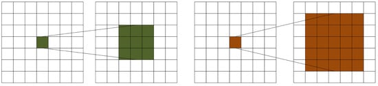
Figure 2.
Different size convolutions correspond to different perceptual fields.
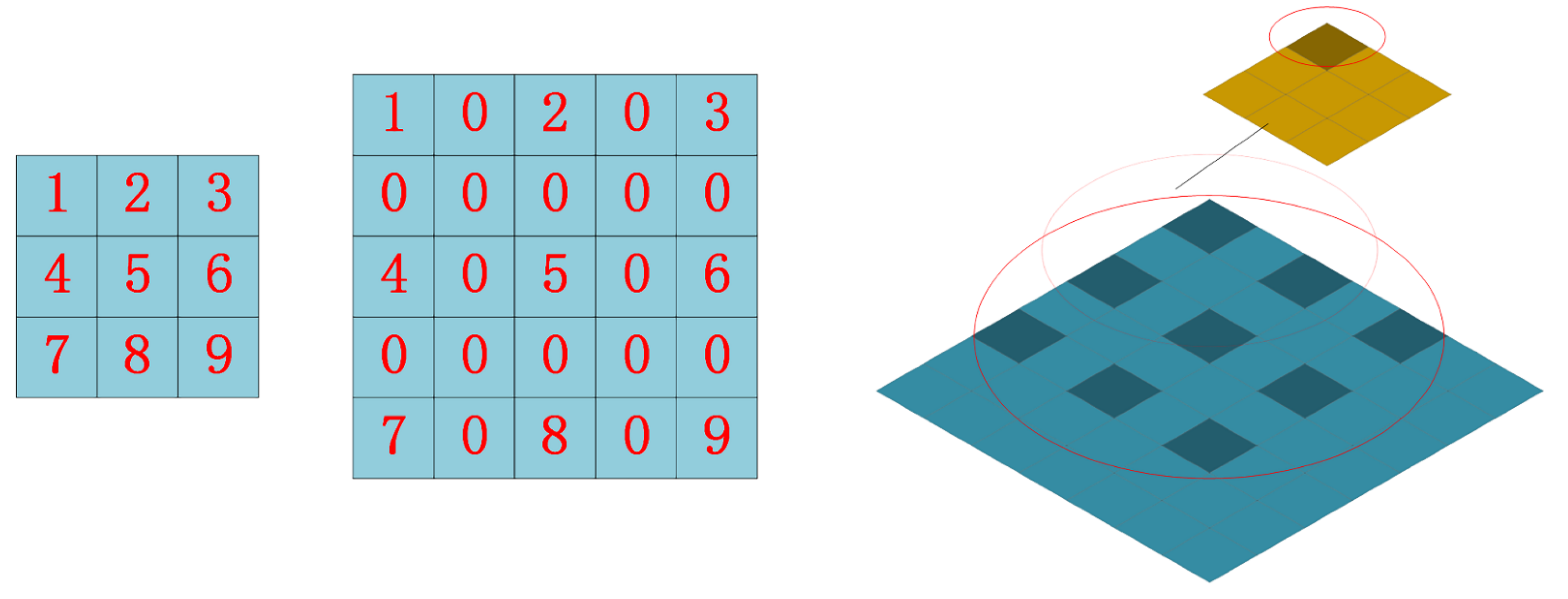
In conclusion, because the particular type of grass had more disturbances, we needed to use more detailed information to distinguish the grass from similar areas. However, the conventional method of expanding the perceptual field would simultaneously cause problems for our model; for this reason, we used the atrous convolution [27]. For segmentation models, when the use of downsampling results in the loss of detailed information and the use of larger convolution kernels results in more parameters, atrous convolution was a new concept to solve these problems. As seen in Figure 3, the original 3 × 3 convolution kernel had a hole added inside of it to increase the field of perception, giving it the same field of perception as a 5 × 5 convolution kernel with the same number of parameters and computational effort (dilated rate = 2), without the use of downsampling. When using atrous convolution, the convolution layer gained a new hyperparameter called the dilated rate, which determined how values were spaced when the convolution kernel processed the data. In this case, the dilated rate was 2. In reality, we added a 0 between each value in the 3 × 3 convolution kernel, separating the values from one another by the original nearby state. A 5 × 5 convolution kernel and the original 3 × 3 convolution shared the same field of perception in this way. It should be mentioned that the standard convolution kernel had a dilation rate of 1.
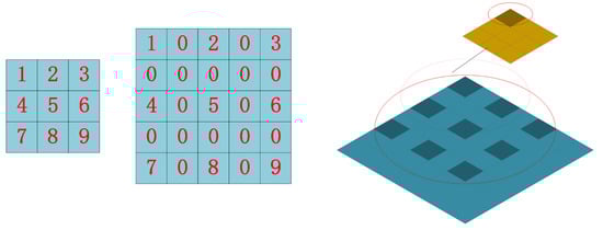
Figure 3.
Atrous convolution display.
Atrous convolution was frequently utilized in semantic segmentation when we needed to capture more detailed information and have limited computational resources.
3.1.2. Backbone Feature Extraction Network MobilnetV2
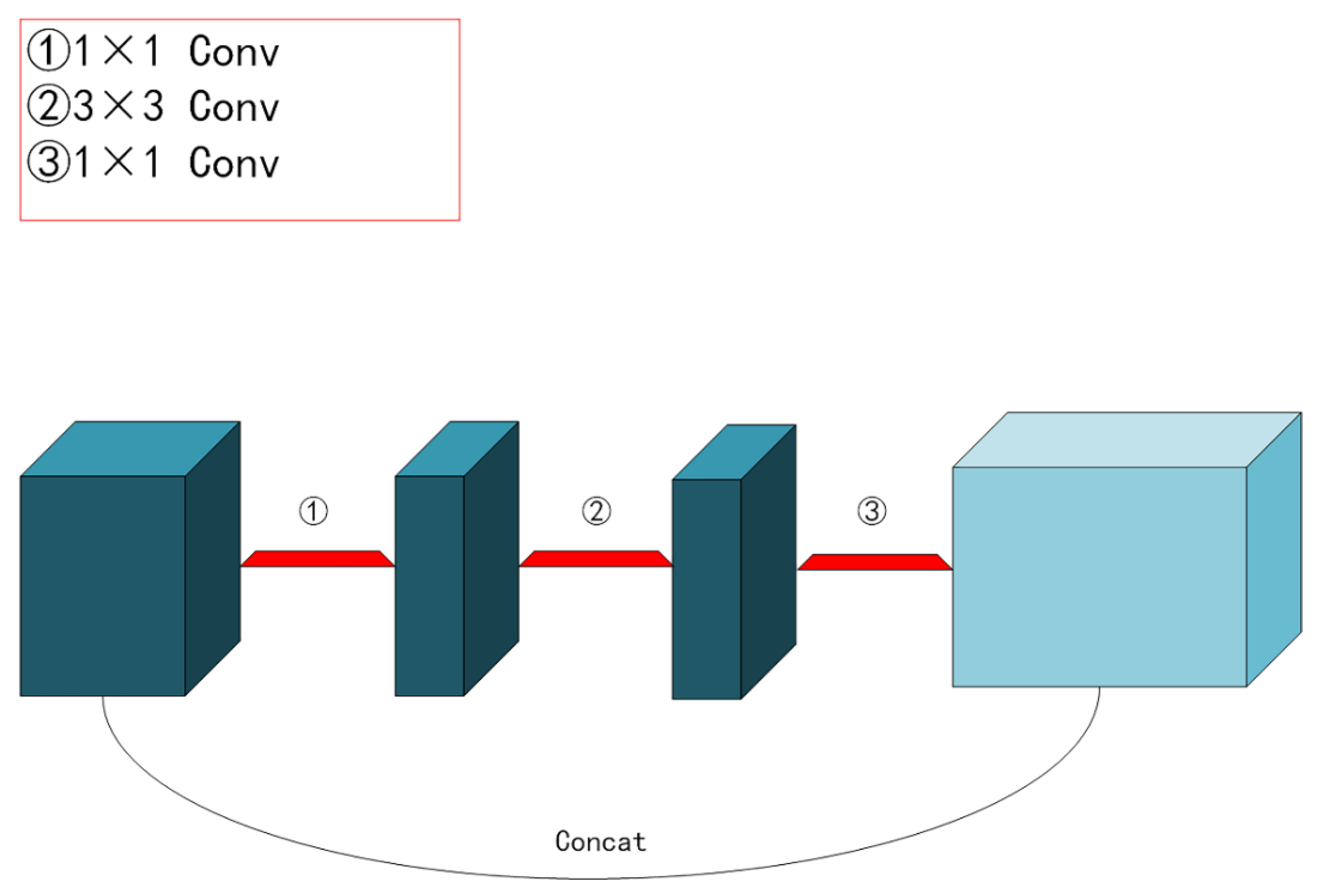
Furthermore, because the number of objects we need to recognize was not finite, we scaled down the backbone feature extraction network and replaced the standard Xception network structure [28] with the lighter mobilnetV2 network structure [29], which further cut down on training time. Explaining the residual and inverse residual structures was required before introducing the mobilnetV2 network topology. According to the traditional residual structure depicted in Figure 4, the initial input was downscaled using a 1 × 1 convolution. Next, features were extracted using a 3 × 3 convolution, upscaled using a 1 × 1 convolution, and finally, the output was produced by splicing the newly created feature layer with the original input. The inverted residual structure in mobilnetV2 used a 1 × 1 convolution to up-dimension the original input, followed by a 3 × 3 deep separable convolutions to extract features, and then a 1 × 1 convolution to downscale. Applying the inverse residual structure would lead to a structure with two tiny ends and a large middle, as seen in Figure 5, as opposed to the original residual structure, which would generate a structure with two large ends and a small middle. Therefore, the essence of the inverted residual structure was why we must first perform the dimensionality increase and then the dimensionality decrease. It goes without saying that if we reduced dimensionality first and subsequently raised it, the 3 × 3 convolution in the middle would require less work. The more computationally costly forms of up-dimensioning and down-dimensioning were used in the mobilnetV2 network topology to enhance feature extraction and produce more valuable features. Deep, separable convolution drastically reduced the number of parameters compared to conventional convolution, ensuring that our computation was not excessively massive even after dimensionality. A single inverse residual structure could not possibly encapsulate the benefits of mobilnetV2, and numerous enhancements were not discussed in this paper. Nevertheless, as seen in Figure 6, the network structure of mobilnetV2 comprises numerous inverse residual structures that were sequentially connected. The mobilnetV2 network was unquestionably lighter than the original Xception network structure utilized in Deeplabv3+, and it significantly increased our training speed.

Figure 4.
Traditional residual structure.
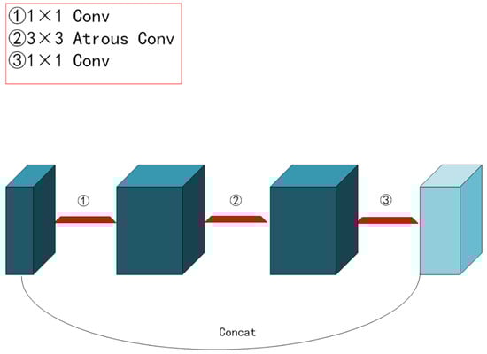
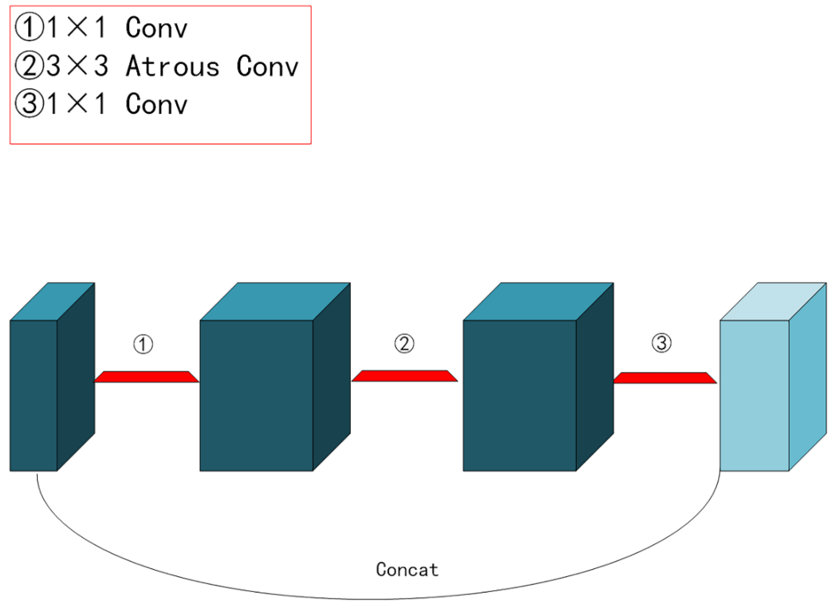
Figure 5.
Inverse residual structure.
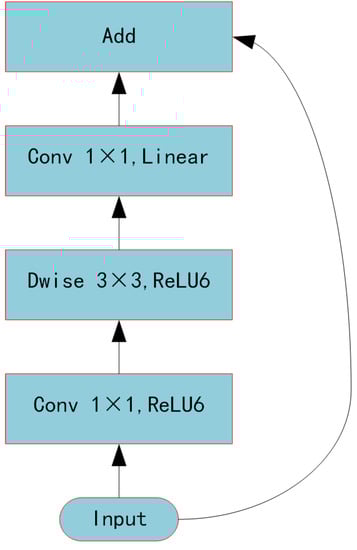
Figure 6.
MobilnerV2 components.
3.1.3. Deeplabv+ Network Structure
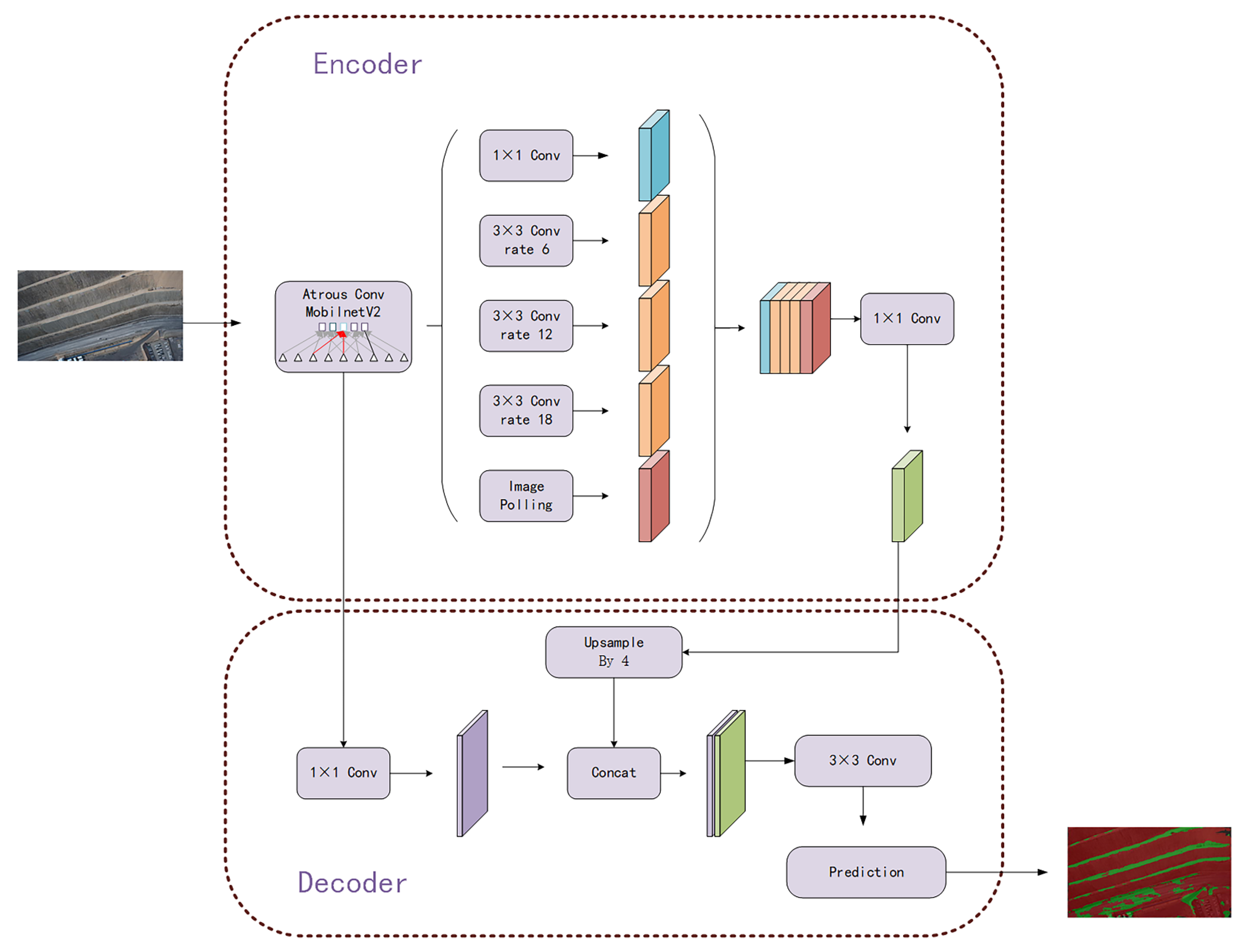
The DeepLabv3+ model [30] had been hailed as a new high point in the evolution of semantic segmentation models. It balanced high- and low-level features extracted by the backbone feature extraction network using atrous convolution, leading to a final feature map that retains the greatest range of feature information, while losing the least amount of detail information. As was noted in the preceding section, the backbone feature extraction portion of the Deeplabv3+ method’s original network structure was Xception. Here, we carried out a large number of experiments and discovered that due to the particularity of the task of grass recognition, when the network structure was too deep and too large, it would increase the recognition effect of the grass, but the overfitting problem would occur. Therefore, we used the mobilnetV2 and the Xception network structure in practice to get almost the same accuracy. However, because the training period for mobilnetV2 was substantially lower than for Xception, we ultimately decided to use mobilnetV2 as our leading feature extraction network. Figure 7 displays our model for segmenting grass. The first stage of encoding and feature extraction and the second stage of decoding and prediction make up the overall network structure. We uniformly resized all training data to 512 × 512 before introducing it into the grass segmentation model. After that, the training data were introduced into the network. (After the backbone feature extraction stage, we retained the original input data results that have been twice and four times compressed.) We convolved the initial adequate feature layers compressed four times with various scales of atrous convolution kernels to generate the feature layers, and then we connected these feature layers, which we refer to as X1. And X1 was then downscaled using the 1 × 1 convolution kernel. The network then moved to the decoding stage. We first utilized 1 × 1 convolution to modify the number of channels of the twice-compressed feature layer generated during the coding stage, which we refer to as X2. Then, in order for the size of the upsampled X1 to match that of X2, we set the up-sampling ratio to 4. The final effective feature layer X was created by stitching the up-sampled X1 and X2 together, and finally, we convolved the X with two atrous convolutions.
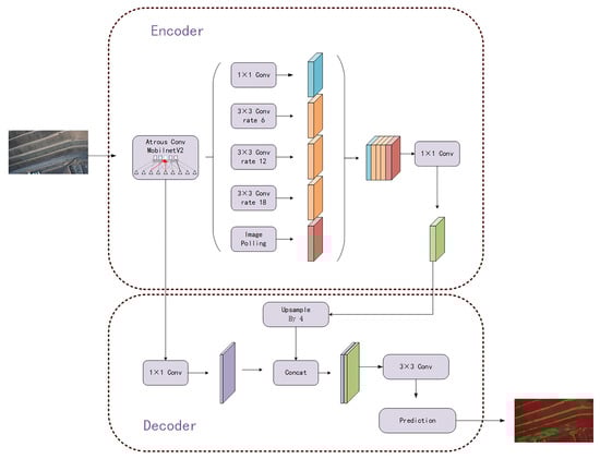
Figure 7.
Grassland division model.
The prediction results could be acquired after the effective feature layer had been obtained after the entire network structure. In order to get the appropriate number of classes (in our trials, we set the number of classes to 4, representing backdrop, grass, road, and water), we first changed the number of channels of X using 1 × 1 convolution. The final prediction result was then obtained by adjusting the output size until it was equal to the size of the input image.
3.2. Vegetation Index Split
The Visible Difference Vegetation Index (VDVI) construction was based on the now widely used Normalised Difference Vegetation Index (NDVI). Fully sensitive to vegetation reflectance and absorption, () replaced the near-infrared band (), combining red () and blue (), (+) replaced the red band () and multiplied the green band by 2 to make it numerically equivalent to + [31]. The vegetation of the VDVI index was highly separated from the non-vegetation, and its values barely intersect. Therefore, it was suitable for vegetation extraction for UAV [32] photography.
where () is the green band, () is the red band, and () is the blue band.
The Otsu algorithm is an algorithm for segmentation by determining the binarization threshold of an image and was proposed by the Japanese scholar Zhenyuki Otsu in 1979 [33]. The Otsu algorithm is the best algorithm for finding the global threshold of an image and is now widely used in image processing.
Two sets of sample plots, A, and B, taken at 128 m, were selected for visual interpretation, and the results of the visual interpretation were calibrated for the vegetation index experiments by field inspection.
4. Results
4.1. Resolution Reconstruction Based on Real-SR Networks
Real-SR was a degradation framework based on kernel estimation and noise injection. Using different degradation combinations (e.g., blur and noise), LR images that shared a common domain with the actual image are obtained. Using this domain-consistent data, an actual image super-resolution Generative Adversarial Networks was trained with a patch discriminator, producing HR results with better perceptual power. Experiments on noisy, synthetic data and authentic images showed that Real-SR outperforms state-of-the-art methods, leading to lower noise and better visual quality. The network did not require paired data for training and can be trained using unlabelled data.
We calculated the PSNR and SSIM of the results generated by different methods after pairing with the experimental data of 192 m flight. PSNR and SSIM are the standard evaluation metrics in image recovery. The PSNR and SSIM were commonly used evaluation metrics in image recovery. These two metrics were more concerned with the fidelity of the images. The metric data were shown in Table 1. The comparison methods include ESRGAN, SRMD, and waifu2x. SRGAN is the first framework to support 4x image magnification, while maintaining a sense of realism. On top of SRGAN, ESRGAN further improves the network structure, loss of resistance, and perception and enhances the image quality of super-resolution processing. Most of the current methods are super-resolution reconstructions for downsampling. SRMD takes low-resolution images of fuzzy cores and noise levels as inputs based on degraded models. WAIFU2X proposed a universal framework with dimensional stretching. WAIFU2X is an extremely commonly used method of lossless super-resolution reconstruction of animated images. It has the characteristics of lightweight and fast processing speed. These three networks have achieved good results in medicine, animation, remote sensing, etc.

Table 1.
Evaluation Metrics.
We evaluated these three methods using the pre-trained models published by the authors. The four methods were also qualitatively analyzed on the Camelot dataset.
ESRGAN lost some of the high-frequency details in the vegetated areas of the green zone in the overscoring. Although it made the image more natural, the difference between vegetation and non-vegetation was reduced. WAIFU2X sharpened the image, but produced noise similar to vegetation, resulting in high vegetation coverage calculated during vegetation extraction. In contrast SRMD and REAL-SR performed better. Figure 8 displays the comparison between these methods. On concrete-covered slopes without vegetation restoration, SRMD had severe texture loss, resulting in blurred images. Both WAIFU2X and ESRGAN were color-biased from the original images, and the textures of WAIFU2X were more different from the original images, while ESRGAN erased almost all detailed textures. Figure 9 displays the comparison. Both SRMD and REAL-SR in the bare ground in the non-green area exhibited a high degree of consistency with the original image, but REAL-SR had a clearer demarcation between the edges of the mound and the bare ground. Figure 10 displays the comparison.
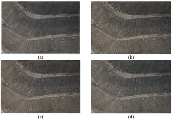
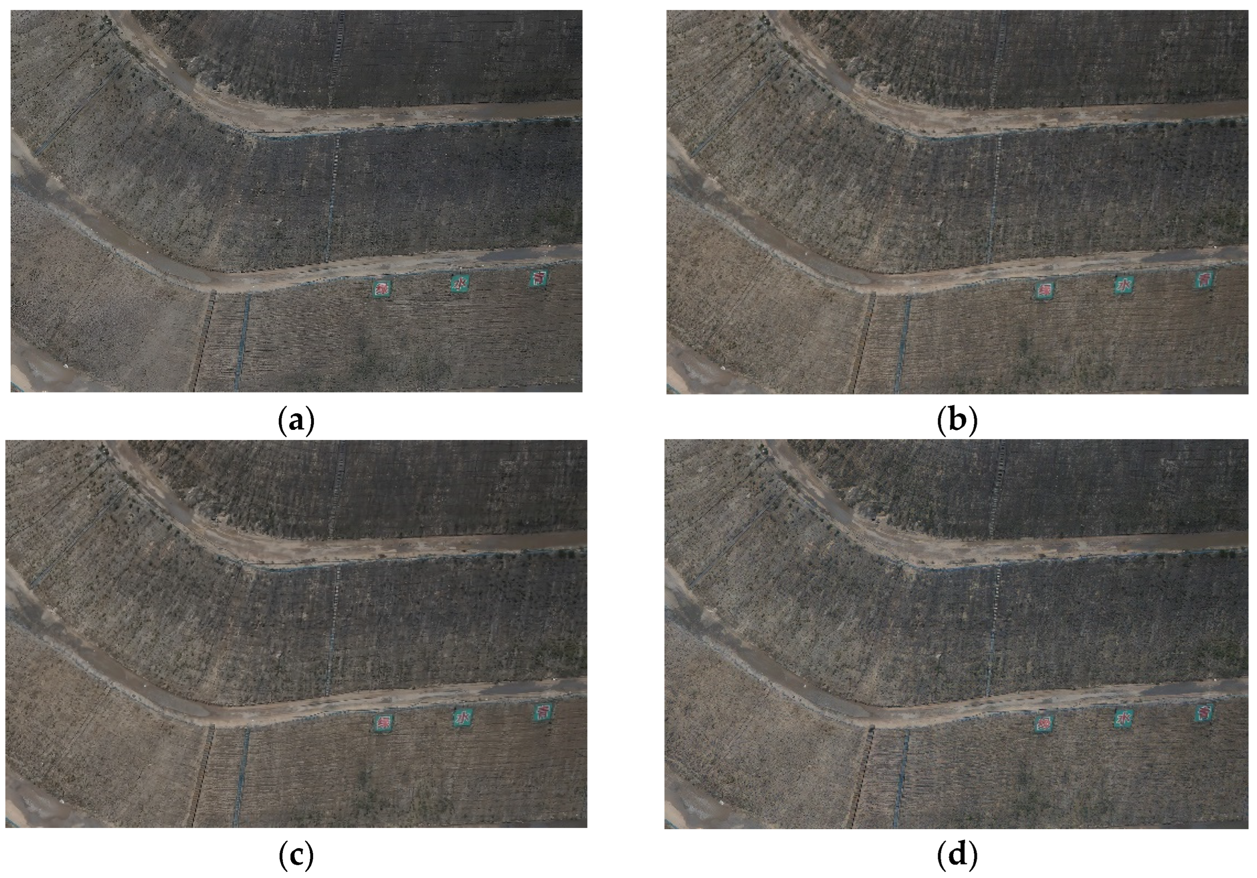
Figure 8.
Comparison of results for green areas (a) ESRGAN, (b) Real-SR, (c) SRMD, (d) WAIFU2X.

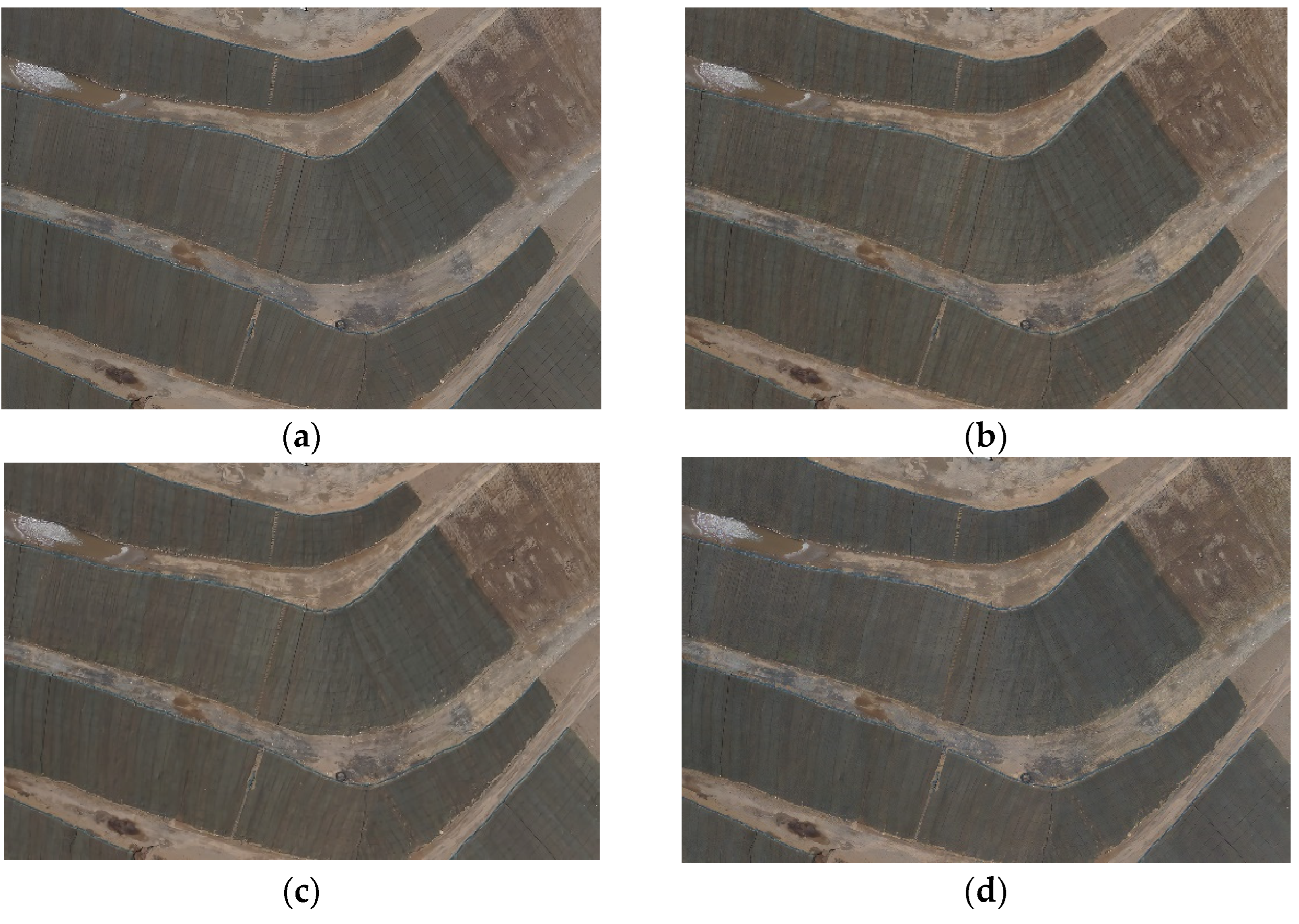
Figure 9.
Comparison of concrete cover results (a) ESRGAN, (b) Real-SR, (c) SRMD, (d) WAIFU2X.
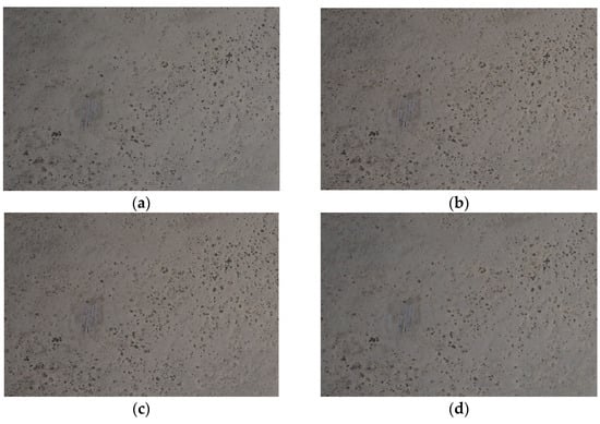
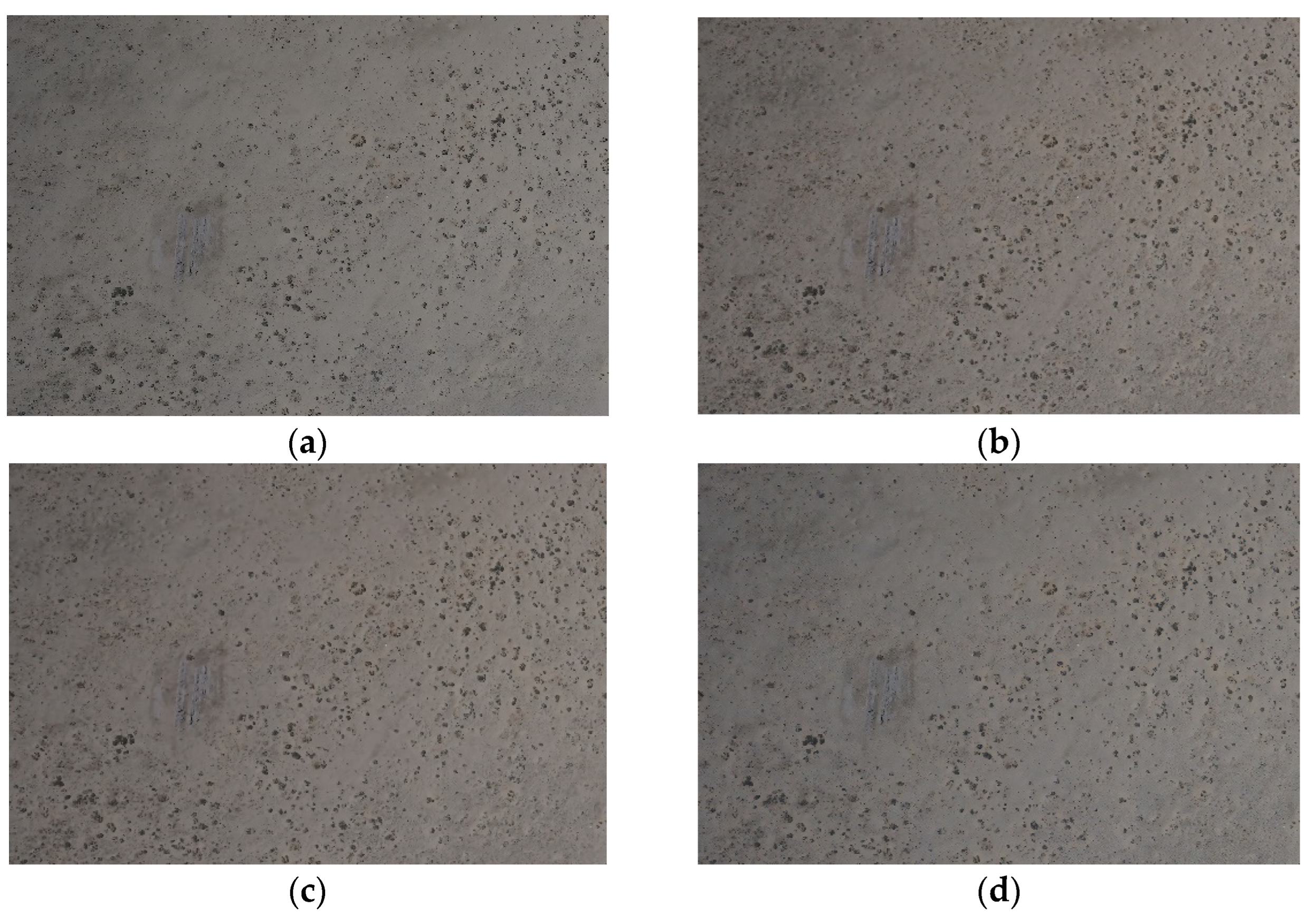
Figure 10.
Comparison of results for bare ground in non-green areas (a) ESRGAN, (b) Real-SR, (c) SRMD, (d) WAIFU2X.
4.2. Ground Segmentation and Interpretation Based on Deeplabv3+ Network
We trained a grass segmentation model based on Deeplabv3+ using the open source deep learning framework TensorFlow, which artificially uses the backbone feature extraction network mobilnetV2 and the atrous convolution approach. An NVIDIA RTX 5000 graphics card and the Ubuntu 18.04 operating system make up our test setup. We used UAV photography first to create a database of mine grass. Then, we used this database to compare the proposed algorithm with some popular algorithms in semantic segmentation and instance segmentation to determine the most effective network model for grass segmentation, and to evaluate the algorithm’s performance. Finally, by altering the fundamental feature-extraction network, the speed of model training was contrasted.
4.2.1. Data Set Creation
The 5697 photos in our dataset were obtained utilizing UAV aerial photography. We photographed many mining locations simultaneously in order to take into account the combined grass cover of multiple mining regions throughout various periods. Considering the various growth conditions that affect grasses in different months, we used drones for three consecutive months to cover the sparse, growing, and mature states of grasses in the dataset. The experiment’s dataset was split into two parts: a training set that made up 90% of the dataset and a test set that made up 10%. In other words, there are 5114 images in the training set and 583 images in the test set. Since there were relatively few water sources in the mining area, not all photos contain water sources. We show a selection of representative photos from the mining region in Figure 11.
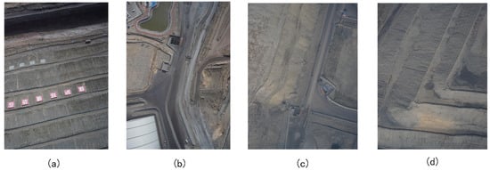
Figure 11.
Some of the more representative images in the dataset. (a) pictures of mining meadows, (b) pictures of the mine road, (c) pictures of mining land, (d) pictures of mining land.
4.2.2. Semantic Segmentation and Instance-Segmentation Selection
In order to choose the best procedure, we first carried out a substantial number of experiments, explicitly comparing the algorithm suggested in the paper with Mask-RCNN, a well-known approach in the field of instance segmentation.
We discovered during the experiments that the prior instance segmentation domain primarily targets single objects, i.e., the individual objects segmented in an image were objects with independent and complete contours, such as people, cars, and dogs, which are distinguished by being relatively small. These objects took up a small amount of space in the image, and had good boundary lines. However, a sizable issue appeared when we employed Mask-RCNN to segment grass. Due to the unique characteristics of grass recognition, grass frequently took up most of an image. A single shot frequently could not capture the entirety of the grass because it was a visible object with a vast surface area. Therefore, the grass took up almost three-quarters of the image. In addition, the grass did not have a distinct outline because it essentially overflows its range of expression in a single image, making it difficult to distinguish from other objects.
Due to the issues above, when using instance segmentation on a grassy area, only a tiny portion of the grass was frequently detected, and it did not include the entire grass area. In addition, the instance segmentation had poor segmentation results for relatively small objects that appear less frequently in the image, such as roads. We employed the semantic segmentation model Deeplabv3+ as our segmentation model to identify the grass in order to address the issues mentioned above. The semantic segmentation tended to segment the image from region to region, in contrast to instance segmentation, which treated grass as a single item. As a result, the segmentation of the grass was smoother, and the semantic segmentation could identify as many of the image’s pixels that belong to the grass as possible.
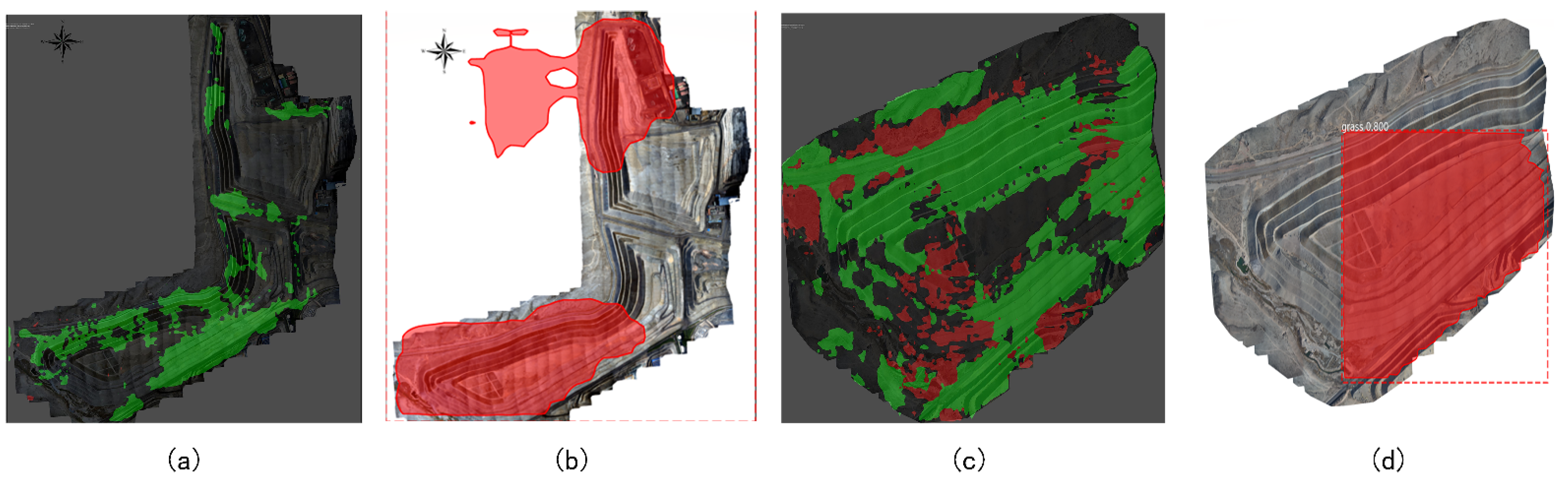
The outcomes of our segmentation of the grass image using Mask-RCNN and the algorithm suggested in the paper are displayed in Figure 12. The area represented by (a) and (b) is the Mengxi drainage field, and the area represented by (c) and (d) is the Luotuo Mountain drainage field, both of which are mining areas at our experimental site. Where (a), (c), and (b), (d) are the outcomes of segmenting an image of grass using the algorithm described in the paper and the Mask-RCNN algorithm, respectively. We can see from the figure that the results of the grass segmentation using the Mask-RCNN algorithm exhibit signs of piecemeal behavior because Mask-RCNN attempts to segments each blade of grass separately. As a result, the whole does not exhibit the continuity that the grass segmentation should have, and the road, which is less prominent and has a different shape from the grass in the image, is not well segmented. The suggested algorithm performs grass segmentation more coherently than the Mask-RCNN algorithm and achieves superior segmentation results for small and irregularly shaped objects.

Figure 12.
Comparison with Mask-RCNN algorithm, (a) results obtained using semantic seg-mentation for the Luotuo Mountain drainage field, (b) results obtained using instance segmentation for the Luotuo Mountain drainage field, (c) results obtained by using semantic segmentation for the Mengxi drainage field, (d) results obtained using instance segmentation for the Mengxi drainage field. The green area in (a,c) represents grass. The red area in (a,c) represents land. The red area in (b,d) represents grass.
4.2.3. Experimental Setup
Evaluation Criteria
We measured the effectiveness of our algorithm on the dataset using three metrics: pixel accuracy PA, category average pixel accuracy MPA, and average cross-merge ratio MIoU. The pixel accuracy PA is the cumulative average of the ratio of correctly classified pixels for each category. MPA is the cumulative average of the ratio of correctly predicted pixels to the total number of pixels for each pixel. And MoU is the cumulative average of the intersection of predicted results and actual results for each category. The following is the calculation for these three measures.
where I represents category I, and I belongs to one of the categories of road, grass, and water, TPi indicates that the model correctly predicts category I as part of category i. Fri indicates that the model incorrectly predicts other categories as part of category i. TNi indicates that the model correctly predicts other categories as part of other categories, and Fri indicates that the model incorrectly predicts the part belonging to category I as not belonging to category I part. Our aim is to obtain a model that makes all three of these metrics higher.
Introducing the Comparison Algorithm
We compared our algorithm with some already-existing, more representative semantic segmentation models based on convolutional neural networks [34,35,36], and the essential details of these approaches, such as the year of publication, the source, the network model obtained with are listed in Table 2. This comparison allowed us to assess our grass-segmentation algorithm properly.
Table 2.
Basic information of the Three algorithms.
Training Parameters
The training parameters are listed in Table 3.
Table 3.
Training parameters.
4.2.4. Research on Detection Speed
Our experiments use the open-source deep-learning framework TensorFlow, and the experimental environment is Ubuntu 18.04 operating system with NVIDIA RTX 5000 graphics card. We modified the backbone feature-extraction network in our studies to speed up the detection process, which improved the algorithm’s performance. In addition, we conducted speed comparison experiments by altering the backbone feature-extraction network Xception to mobilnetV2.
Table 4 and Table 5 contain the specifics of the speed comparison. We tested the speed of training an epoch of the backbone feature-extraction network using mobilnetV2 and Xception, respectively, where we set the dataset for speed detection to contain 298 images in order to examine the change in speed and performance of the algorithm after the modification of the backbone feature extraction network. As shown in Table 5 and Table 6, training an epoch with mobilnetV2 and Xception took different amounts of time. On the speed comparison dataset, training one epoch takes 84 s for mobilnetV2 and 498 s for Xception. Although the more profound framework Xception slightly improves the results, a sizable amount of time is lost, and we do not think the performance improvement makes up for the time lost. As a result, our primary feature extraction network is mobilnetV2.
Table 4.
The comparisons of detection speed in our dataset.
Table 5.
The comparisons of performance with different backbone.
Table 6.
The overall experimental results in our dataset.
4.2.5. Comparison with Other Semantic Segmentation Methods in Terms of Performance
Using our established grass dataset and comparison metrics, including PA, MPA, and MoU, we compared our proposed method against other neural network-based semantic segmentation techniques, such as SegNet [34], Deeplab [35], and FCN [36]. We conducted the grass-segmentation experiments using fixed partitions for the training and test sets.
4.2.6. Overall Experimental Results
Table 6 shows that the authors’ SegNet network for semantic segmentation in [34] performs well on our grass segmentation dataset, with an accuracy rate slightly higher than 72 percent and MPA and MoU values reaching 55.34 percent and 44.23 percent, respectively. In general, the method suggested in [34] is the most applicable of these three methods for our dataset. The method proposed in [36] also performs slightly worse on our dataset than in [34], with an accuracy rate of only 70.45 percent and the second highest MPA value among these three methods, reaching 53.68 percent. However, its MoU value is the lowest among these three methods. We speculate that this is because the method’s relatively weak feature extraction of detailed information makes it more likely to cause a problem when segmenting. Overall, the method in [36] has good performance in these two metrics for our dataset, but its MPA value is the worst among the three methods, with only 51.07 percent, which we found unsatisfactory. The accuracy rate of the method proposed by the authors in [36] is the second highest among the three methods with 71.80 percent, and the MoU value is the first among the three methods with 44.82 percent. We hypothesize that this is because the segmentation effect of the method in [36] is better only for larger objects and worse for some more minor things. Table 6 shows that our suggested method exceeds the method in [34,35,36] in each of the three metrics, with values of 78.71%, 55.69%, and 45.24%, respectively. The approach is the most effective in Table 6 for all metrics, and we think that achieving such metrics for items such as grass that are more challenging to segment is a more satisfying outcome for our approach. One reason is that we use various cavity convolution sizes in the network model, which enables the feature extraction stage to access additional feature information and specifics.
Additionally, this is because our network model performs feature fusion in two stages: first, after the atrous convolution of multiple scales, and second, in the decoding stage, when the feature map recently extracted from the backbone feature extraction network is fused with the encoding result once more. This preserves the image’s detailed information, while also including the image’s high-level semantic information. This improves the performance of our method for segmenting grass since it keeps not only the image’s granular information, but also its high-level semantic information.
Experimental Results Demonstration
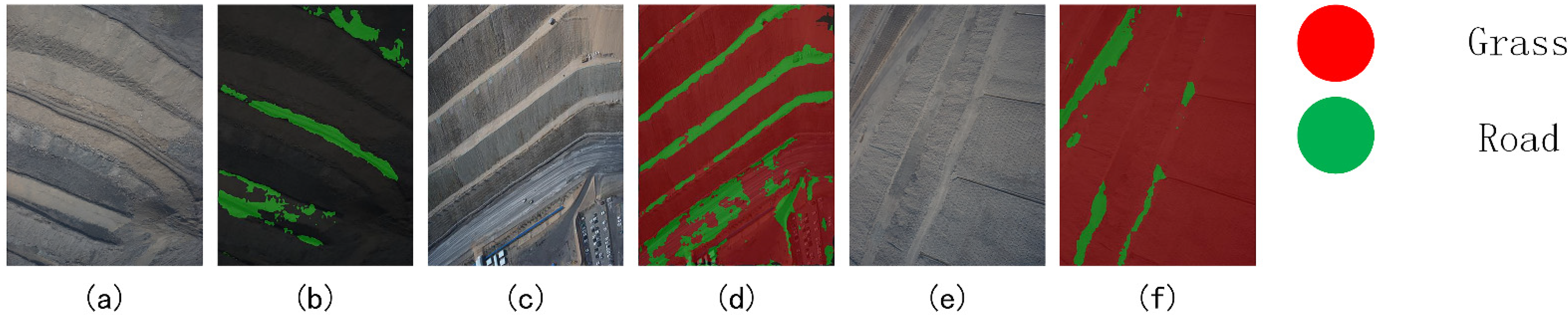
Figure 13 depicts our chosen three representative images, indicating more negligible, moderate, and more vegetation. The images in (a) and (b) show scenes with less vegetation, (c) and (d) show scenes with intermediate vegetation, and (e) and (f) show scenes with more excellent vegetation.
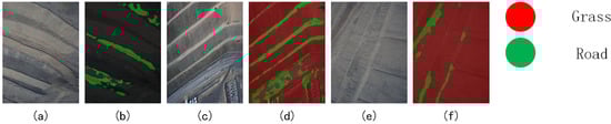
Figure 13.
Demonstration of the effect of the algorithm proposed in the paper on various types of grass, (a) pictures of mining areas with less grassland, (b) the effect of the algorithm proposed in the paper on (a,c) pictures of moderate grassland mining areas, (d) the effect of the algorithm proposed in the paper on (c,e) pictures of mining areas with more grassland, (f) the effect of the alforithm proposed in the paper on (e).
We can see from the Figure 13 that our algorithm has good detection performance for cases of low, moderate, and high levels of vegetation. We can also see that our algorithm has good segmentation performance for these small objects when there is a high level of vegetation and a low level of other categories of objects in images.
4.3. Vegetation Index Splitting Experiments
The results of vegetation extraction using the Otsu method to segment vegetation areas in the greyscale images of four standard visible vegetation indices, namely EXG, EXGR, NGRDI, and RGRI, and the results of the support vector machine and k-mean clustering methods are shown in Figure 13. The SVM and K-means methods are applied directly on drone aerial images. The results of visual interpretation were used as reference maps to calculate the accuracy of vegetation extraction and to analyze the effect of visible vegetation-index extraction. The obtained accuracy evaluation is shown in Table 7.
Table 7.
Accuracy Evaluation.
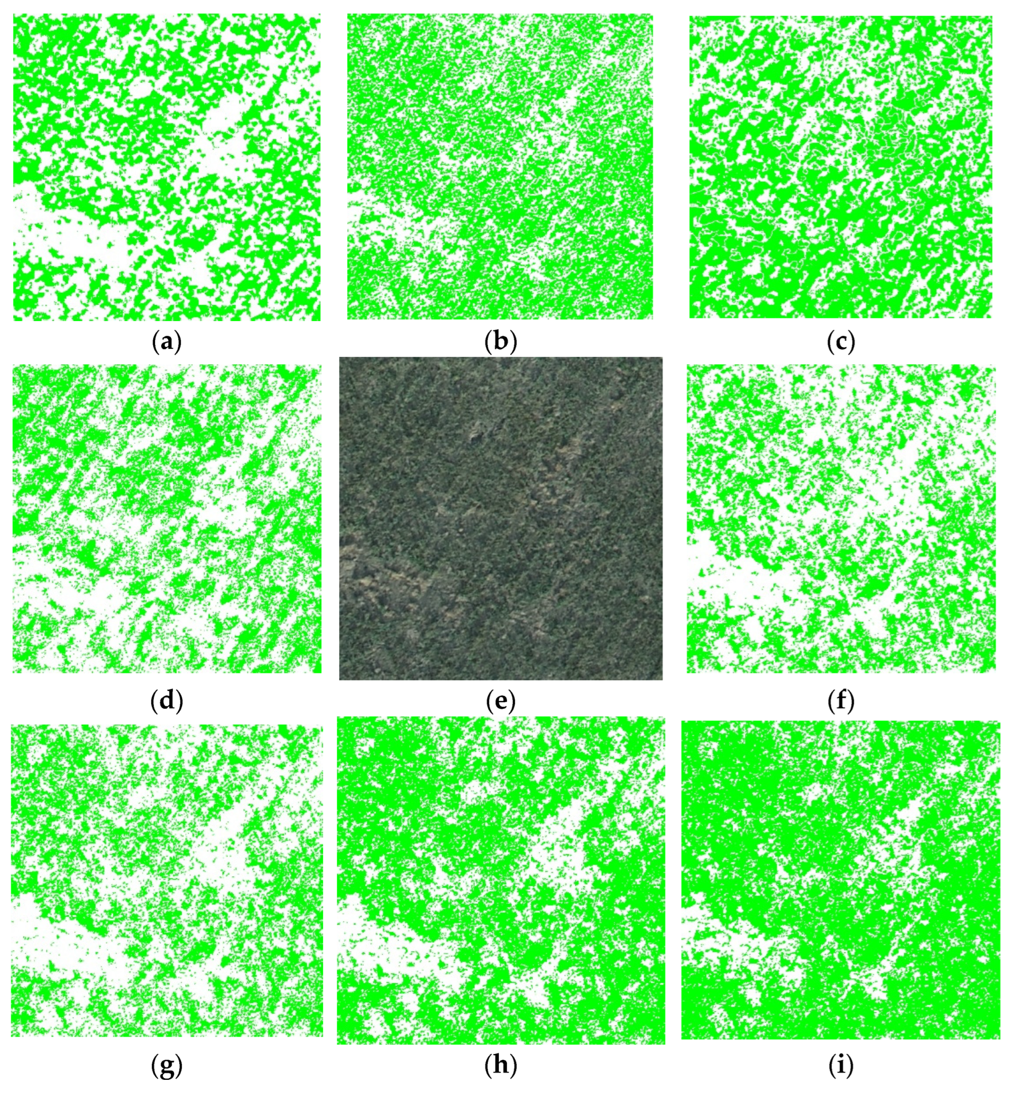
The results in Figure 14 show that the EXG and VDVI vegetation indices have better vegetation segmentation results and are closer to the manual visual interpretation reference results. However, some misclassification of bare ground into vegetation occurs in both indices, while the segmentation results of the EXGR and NGRDI vegetation indices are significantly lower than the other indices. Comparing the supervised classification results with the manual visual-interpretation reference map, it can be concluded that the support vector machine classification results are close to the visual interpretation results. The extraction results are better than the commonly visible vegetation indices. However, there are some misclassification phenomena in some areas, making the support vector machine classification results more significant than the reference results. Comparing the vegetation index segmentation method with the k-means clustering method, it can be seen that the overall misclassification of vegetation index segmentation is less frequent.
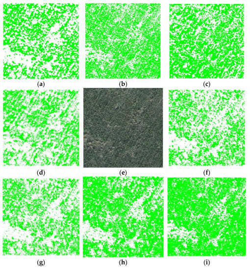
Figure 14.
Comparison of the results of the vegetation extraction in Sample Site A, with vegetation in green. (a) EXG, (b) EXGR, (c) k-mean, (d) NGBDI, (e) RGB, (f) NGRDI, (g) VDVI, (h) truth, (i) svm.
As can be seen from Table 7, among the visible vegetation indices, the VDVI index has the highest recognition accuracy, with an average of 87.10% and a kappa coefficient of 0.764. The NGRDI index also has a high recognition accuracy, with an average of 84.55% and a kappa coefficient of 0.692, while the other visible vegetation indices have relatively low recognition accuracy and the segmentation results are somewhat different. Although the support vector machine has higher segmentation accuracy, the supervised classification is less automated, more complicated to operate, and more dependent on manual work. Based on the above experimental results, it is concluded that VDVI vegetation indices with the OTSU segmentation method can efficiently segment the gangue mountain vegetation.
4.4. More Results
We tested the strategy suggested in the paper on two other mining sites—the Munshi drainage site and the Mengtai drainage site—and we can see from Figure 15 that it is equally effective for all.
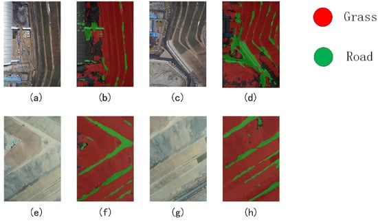
Figure 15.
Application of the method proposed in the paper on other mining sites, where (a–d) are the original and result maps of the Munshi drainage field, and (e–h) are the original and result maps of the Mengtai drainage field.
5. Conclusions
This paper presents a set of methods for ground interpretation of high-altitude UAV visible remote-sensing data based on open drainage sites in northwest China. Super-resolution reconstruction and ground interpretation of remote-sensing images can be unsupervised. UAV aerial mapping has the advantages of high imaging quality and inexpensive site requirements. However, when applied to mines in western Inner Mongolia, the aircraft frequently goes out of control due to the large ground undulations, the high frequency of UAVs going back and forth, and the ease of signal loss. However, acquiring high-resolution images is significant for monitoring vegetation growth, road and water conditions, etc. Overcoming the limitations of imaging sensors is time-consuming and extremely expensive, thus making image super-resolution (SR) technology a viable and economical way to improve the resolution of remote sensing images.
In this paper, the champion algorithm of the NTIRE 2020 challenge was chosen to be trained with low-altitude, high-resolution images. Compared to traditional super-resolution reconstruction methods, real-sr does not require complex labeling of the images. Moreover, after training, its similarity to the original image is high. However, it is limited by the small number of training samples, the small noise pool, and the different ground cover textures. This results in a large gap between some textured features extracted as noise and then returned to the original features. However, all in all, using super-resolution reconstruction in remote effectively reduces the aircraft failure rate, thus significantly improving efficiency. The high flight altitude ensures that the aircraft’s GPS signal is not affected by the massive mountain ups and downs. The problem of hover instability and automatic return failure is avoided, and the safety of the UAV is improved.
With the continuous development of deep learning in recent years, its application in remote sensing is becoming more widespread. Green area image segmentation is of great importance for the reconstruction of mine development, and the performance of the green area segmentation model depends very much on whether the detailed information about the grass in the image can be extracted. This paper innovatively uses the labv3+network+vegetation index segmentation method to first segment roads, water bodies that are easily confused during vegetation index extraction, green areas with only vegetation and bare ground, and non-green areas. The vegetation extraction of the two areas is then carried out to more concretely represent the differences in vegetation cover between green and non-green areas. Multi-layer classification methods are often more effective when interpreting remote sensing in the face of complex landscapes than single classification networks. Some traditional segmentation methods can work better than deep-learning methods when faced with specific situations.
In this paper, DeepLabv3+ was improved and successfully applied to grass segmentation with relatively good results. The experimental results show that our model achieves reliable results in grass recognition compared with classical semantic segmentation models such as FCN, SegNet, etc. However, the mining data is relatively challenging to collect, resulting in the training quality will be limited by the data, and the similarity of green area in the image with non-green areas is also a key factor limiting the performance of our algorithm, which is also our main research direction in the future.
Author Contributions
Y.W.: Conceptualization, Writing—review and editing, Supervision. D.Y.: Methodology, Software, Formal analysis, Writing—original draft. L.L.: Conceptualization, Writing—review and editing. X.L.: Supervision, Investigation, Data curation. P.C.: Resources. Y.H.: Visualization, Project administration. All authors have read and agreed to the published version of the manuscript.
Funding
This study was financially supported by the Science and Technology Major Project of Inner Mongolia Autonomous Region (Grant No. 2020ZD0021).
Data Availability Statement
Not applicable.
Conflicts of Interest
The authors declare no conflict of interest.
References
- Shen, H.; Ng, M.K.; Li, P.; Zhang, L. Super-resolution reconstruction algorithm to MODIS remote sensing images. Comput. J. 2009, 52, 90–100. [Google Scholar] [CrossRef]
- Qifang, X.; Guoqing, Y.; Pin, L. Super-resolution reconstruction of satellite video images based on interpolation method. Procedia Comput. Sci. 2017, 107, 454–459. [Google Scholar] [CrossRef]
- Ding, H.; Bian, Z. Remote Sensed Image Super-Resolution Reconstruction Based on a BP Neural Network. Comput. Eng. Appl. 2008, 44, 171–172. [Google Scholar]
- Wen, C.; Yuan-fei, W. A Study on A New Method of Multi-spatial-resolution Remote Sensing Image Fusion Based on GA—BP. Remote Sens. Technol. Appl. 2011, 22, 555–559. [Google Scholar]
- Ma, W.; Pan, Z.; Guo, J.; Lei, B. Achieving super-resolution remote sensing images via the wavelet transform combined with the recursive res-net. ITGRS IEEE Trans. Geosci. Remote Sens. 2019, 57, 3512–3527. [Google Scholar] [CrossRef]
- Jalonen, J.; Järvelä, J.; Virtanen, J.-P.; Vaaja, M.; Kurkela, M.; Hyyppä, H. Determining characteristic vegetation areas by terrestrial laser scanning for floodplain flow modeling. Water 2015, 7, 420–437. [Google Scholar] [CrossRef]
- Yaseen, Z. An insight into machine learning models era in simulating soil, water bodies and adsorption heavy metals: Review, challenges and solutions. Chemosphere 2021, 277, 130126. [Google Scholar] [CrossRef]
- Khan, M.A.; Sharma, N.; Lama, G.F.C.; Hasan, M.; Garg, R.; Busico, G.; Alharbi, R.S. Three-Dimensional Hole Size (3DHS) Approach for Water Flow Turbulence Analysis over Emerging Sand Bars: Flume-Scale Experiments. Water 2022, 14, 1889. [Google Scholar] [CrossRef]
- Lama, G.; Errico, A.; Pasquino, V.; Mirzaei, S.; Preti, F.; Chirico, G. Velocity Uncertainty Quantification based on Riparian Vegetation Indices in open channels colonized by Phragmites australis. J. Ecohydraulics 2022, 7, 71–76. [Google Scholar] [CrossRef]
- Kutz, J.N. Deep learning in fluid dynamics. JFM J. Fluid Mech. 2017, 814, 1–4. [Google Scholar] [CrossRef]
- Shen, C. A transdisciplinary review of deep learning research and its relevance for water resources scientists. WRR Water Resour. Res. 2018, 54, 8558–8593. [Google Scholar] [CrossRef]
- Huete, A.; Didan, K.; Miura, T.; Rodriguez, E.P.; Gao, X.; Ferreira, L.G. Overview of the radiometric and biophysical performance of the MODIS vegetation indices. Remote Sens. Environ. 2002, 83, 195–213. [Google Scholar] [CrossRef]
- Torres-Sánchez, J.; Peña, J.M.; de Castro, A.I.; López-Granados, F. Multi-temporal mapping of the vegetation fraction in early-season wheat fields using images from UAV. Comput. Electron. Agric. 2014, 103, 104–113. [Google Scholar] [CrossRef]
- Hong, J.; Xiaoqin, W.; Bo, W. A topographyadjusted vegetation index (TAVI) and its application in vegetation fraction monitoring. J. Fuzhou Univ. Nat. Sci. Ed. 2010, 38, 527–532. [Google Scholar]
- Meyer, G.E.; Neto, J.C. Verification of color vegetation indices for automated crop imaging applications. Comput. Electron. Agric. 2008, 63, 282–293. [Google Scholar] [CrossRef]
- Natesan, S.; Armenakis, C.; Vepakomma, U. Resnet-Based Tree Species Classification Using Uav Images. ISPRS Int. Arch. Photogramm. Remote Sens. Spat. Inf. Sci. 2019, 4213, 475–481. [Google Scholar] [CrossRef]
- Yang, J.Y.; Zhou, Z.X.; Du, Z.R.; Xu, Q.Q.; Yin, H.; Liu, R. Extraction of rural construction land from high-resolution remote sensing images based on SegNet semantic model. Chin. J. Agric. Eng. 2019, 35, 251–258. [Google Scholar]
- Lobo Torres, D.; Queiroz Feitosa, R.; Nigri Happ, P.; Elena Cué La Rosa, L.; Marcato Junior, J.; Martins, J.; Olã Bressan, P.; Gonçalves, W.N.; Liesenberg, V. Applying fully convolutional architectures for semantic segmentation of a single tree species in urban environment on high resolution UAV optical imagery. Sensors 2020, 20, 563. [Google Scholar] [CrossRef]
- Wang, C.H.; Zhao, Q.Z.; Ma, Y.J.; Ren, Y.Y. Crop Classification by UAV Remote Sensing Based on Convolutional Neural Network. J. Agric. Mach. 2019, 50, 161–168. [Google Scholar]
- Zhou, C.; Ye, H.; Xu, Z.; Hu, J.; Shi, X.; Hua, S.; Yue, J.; Yang, G. Estimating maize-leaf coverage in field conditions by applying a machine learning algorithm to UAV remote sensing images. Appl. Sci. 2019, 9, 2389. [Google Scholar] [CrossRef]
- Long, J.; Shelhamer, E.; Darrell, T. Fully convolutional networks for semantic segmentation. In Proceedings of the IEEE Conference on Computer Vision and Pattern Recognition, Boston, MA, USA, 6–8 June 2015. [Google Scholar]
- Morales, G.; Kemper, G.; Sevillano, G.; Arteaga, D.; Ortega, I.; Telles, J. Automatic segmentation of Mauritia flexuosa in unmanned aerial vehicle (UAV) imagery using deep learning. Forests 2018, 9, 736. [Google Scholar] [CrossRef]
- Ji, X.; Cao, Y.; Tai, Y.; Wang, C.; Li, J.; Huang, F. Real-world super-resolution via kernel estimation and noise injection. In Proceedings of the IEEE/CVF Conference on Computer Vision and Pattern Recognition Workshops, Seattle, WA, USA, 14–19 June 2020. [Google Scholar]
- Wang, X.; Yu, K.; Wu, S.; Gu, J.; Liu, Y.; Dong, C.; Qiao, Y.; Change Loy, C. Esrgan: Enhanced super-resolution generative adversarial networks. In Proceedings of the European Conference on Computer Vision (ECCV) Workshops, Munich, Germany, 10–14 September 2018. [Google Scholar]
- Dong, C.; Loy, C.C.; He, K.; Tang, X. Image super-resolution using deep convolutional networks. IEEE Trans. Pattern Anal. Mach. Intell. 2015, 38, 295–307. [Google Scholar] [CrossRef] [PubMed]
- Zhang, K.; Zuo, W.; Zhang, L. Learning a single convolutional super-resolution network for multiple degradations. In Proceedings of the IEEE Conference on Computer Vision and Pattern Recognition, Salt Lake City, UT, USA, 18–23 June 2018. [Google Scholar]
- Yu, F.; Koltun, V. Multi-scale context aggregation by dilated convolutions. arXiv 2015, arXiv:1511.07122. [Google Scholar]
- Chollet, F. Xception: Deep learning with depthwise separable convolutions. In Proceedings of the IEEE Conference on Computer Vision and Pattern Recognition, Honolulu, HI, USA, 21–26 July 2017. [Google Scholar]
- Sandler, M.; Howard, A.; Zhu, M.; Zhmoginov, A.; Chen, L.-C. Mobilenetv2: Inverted residuals and linear bottlenecks. In Proceedings of the IEEE Conference on Computer Vision and Pattern Recognition, Salt Lake City, UT, USA, 18–23 June 2018. [Google Scholar]
- Chen, L.-C.; Zhu, Y.; Papandreou, G.; Schroff, F.; Adam, H. Encoder-decoder with atrous separable convolution for semantic image segmentation. In Proceedings of the European Conference on Computer Vision (ECCV), Munich, Germany, 8–14 September 2018. [Google Scholar]
- Zhou, Z.; Yang, Y.; Chen, B. Study on the extraction of exotic species Spartina alterniflora from UAV visible images. J. Subtrop. Resour. Environ. 2017, 12, 90–95. [Google Scholar]
- Gao, Y.; Kang, M.; He, M.; Sun, Y.; Xu, H. Extraction of desert vegetation coverage based on visible light band information of unmanned aerial vehicle: A case study of Shapotou region. J. Lanzhou Univ. Nat. Sci. 2018, 54, 770–775. [Google Scholar]
- Gonzalez, R.C. Digital Image Processing; Pearson Education India: Noida, India, 2009. [Google Scholar]
- Badrinarayanan, V.; Kendall, A.; Cipolla, R. Segnet: A deep convolutional encoder-decoder architecture for image segmentation. IEEE Trans. Pattern Anal. Mach. Intell. 2017, 39, 2481–2495. [Google Scholar] [CrossRef]
- Chen, L.; Papandreou, G.; Kokkinos, I.; Murphy, K.; Yuille, A. DeepLab: Semantic Image Segmentation with Deep Convolutional Nets, Atrous Convolution, and Fully Connected CRFs. IEEE Trans. Pattern Anal. Mach. Intell. 2017, 40, 834–848. [Google Scholar] [CrossRef]
- Shelhamer, E.; Long, J.; Darrell, T. Fully Convolutional Networks for Semantic Segmentation. IEEE Trans. Pattern Anal. Mach. Intell. 2017, 39, 640–651. [Google Scholar] [CrossRef]


Publisher’s Note: MDPI stays neutral with regard to jurisdictional claims in published maps and institutional affiliations. |
© 2022 by the authors. Licensee MDPI, Basel, Switzerland. This article is an open access article distributed under the terms and conditions of the Creative Commons Attribution (CC BY) license (https://creativecommons.org/licenses/by/4.0/).