Mutual Guidance Meets Supervised Contrastive Learning: Vehicle Detection in Remote Sensing Images

Abstract

Vehicle detection is an important but challenging problem in Earth observation due to the intricately small sizes and varied appearances of the objects of interest. In this paper, we use these issues to our advantage by considering them results of latent image augmentation. In particular, we propose using supervised contrastive loss in combination with a mutual guidance matching process to helps learn stronger object representations and tackles the misalignment of localization and classification in object detection. Extensive experiments are performed to understand the combination of the two strategies and show the benefits for vehicle detection on aerial and satellite images, achieving performance on par with state-of-the-art methods designed for small and very small object detection. As the proposed method is domain-agnostic, it might also be used for visual representation learning in generic computer vision problems.

1. Introduction

Object detection consists of two tasks: localization and classification. As they are different in nature [1] yet contribute toward the overall detection performance, deep architectures usually have two distinct prediction heads, which share the same features extracted from an input. The separated branches, despite the shared parameters, have shown inefficiency as classification scores might not well reflect proper localization [2,3], while the intersection-over-union (IOU) scores of anchor boxes might miss the semantic information [4].

The misalignment of localization and classification may be aggravated depending on the domain of application. Vehicle detection is a challenging but important problem in Earth observation. It is instrumental for traffic surveillance and management [5], road safety [6], traffic modeling [7], and urban planning [8] due to large coverage from aerial viewpoints [9]. The intrinsic challenges include, but are not limited to, the small and diverse sizes of vehicles, inter-class similarity, illumination variation, and background complexity [10,11].

A simple method to combine the localization and classification score to mutually guide the training process, recently introduced by Zhang et al. [4], has shown effectiveness in alleviating the task misalignment problem on generic computer vision datasets MS-COCO [12] and PASCAL-VOC [13]. Its ability to cope with the intricacies of remote sensing vehicle detection yet remains unexplored.

In this paper, we propose a framework inspired by the mutual guidance idea [4] for vehicle detection from remote sensing images (Figure 1). The idea is that the intersection-over-union (IOU) of an anchor box should contribute toward the predicted category and vice versa; the learned semantic information could help in providing more fitting bounding boxes.

Figure 1. Vehicle detection from the VEDAI’s aerial images performed by the proposed contrastive mutual guidance loss. Class labels include car (1), truck (2), pickup (3), tractor (4), camping (5), boat (6), van (7), other (8).

To improve the semantic understanding and overcome the varied object sizes and appearances, we also propose a loss module based on the contrastive learning notion [14,15]: for each detected object, the other objects of the same class are pulled closer in the embedding space, while those of different classes are pushed away. The underlying intuition is that the features of the same-class objects should be close together in the latent space, and by explicitly imposing this, the network is forced to learn representations that better underline intra-class characteristics.

Contrastive learning is a discriminative approach to visual representation learning, which has proven effective for pre-training networks before transferring to an actual downstream task [16,17,18,19,20]. The well-known SimCLR framework [16] proposes applying image augmentation to create an image’s positive counterpart, eliminating the need for manual annotations for pretext tasks, hence self-supervision. Our hypothesis is that different objects of the same class from aerial points of view could be considered as a result of compositions of multiple augmentation operations, such as cropping, scaling, re-coloring, adding noises, etc., which, as shown by SimCLR, should be beneficial for representation learning (Figure 2). Thus, by pulling together same-class objects and pushing away the others, the network could learn to overcome the environmental diversity and better recognize the objects of interest.

Figure 2. Different objects of the same class, “car”, from an aerial point of view could be considered as passing through various compositions of image augmentation, such as cropping, rotation, re-coloring, noise adding, etc.

As we rely on ground truth labels to form positive and negative contrastive pairs, the proposed contrastive loss could be seen as being inspired by supervised contrastive learning [17], but applied here to object detection. The differences are that the contrastive pairs are drawn from object-instance level, not image level, and that contrastive loss is employed as an auxiliary loss in combination with the mutually guided detection loss.

The contributions of the paper are fourfold, i.e.,

• applying the mutual guidance idea to a remote sensing context;
• formulating supervised contrastive learning as an auxiliary loss in a detection problem, which, to the best of our knowledge, is the first approach using supervised contrastive learning for object detection, especially in the context of Earth observation;
• improving existing detection networks for vehicle detection by combining mutual guidance and contrastive learning, termed contrastive mutual guidance or CMG;
• providing new state-of-the-art results on benchmarked datasets including VEDAI (aerial images) [21] and xView (satellite images) [22].

2. Related Work

2.1. Vehicle Detection in Remote Sensing

Deep-learning-based vehicle detection from aerial and satellite images has been an active research topic in remote sensing for Earth observation within the last decade due to intrinsically challenging natures such as intricately small vehicle sizes, various types and orientations, heterogeneous backgrounds, etc. General approaches include adapting state-of-the-art detectors from the computer vision community to apply to Earth observation context [11,23,24]. Similar to the general object detection task [25], most of the proposed methods could be divided into one-stage and two-stage approaches and are generally based on anchor box prediction. Famous anchor-based detector families such as Faster-RCNN, SSD, and YOLO have been widely exploited in remote sensing object detection, including vehicles. In [26,27], the authors proposed to modify and improve the Faster-RCNN detector for vehicle detection from aerial remote sensing images. Multi-scaled feature fusion and data augmentation techniques such as oversampling or homography transformation have proven to help two-stage detectors to provide better object proposals.

In [28,29], YOLOv3 and YOLOv4 were modified and adapted to tackle small vehicle detection from both Unmanned Aerial Vehicle (UAV) and satellite images with the objective of providing a real-time operational context. In the proposed YOLO-fine [28] and YOLO-RTUAV [29] models, the authors attempted to remove unnecessary network layers from the backbones of YOLOv3 and YOLOv4-tiny, respectively, while adding some others to focus on small object searching. In [23], the Tiramisu segmentation model as well as the YOLOv3 detector were experimented and compared for their capacity to detect very small vehicles from 50-cm Pleiades satellite images. The authors finally proposed a late fusion technique to obtain the combined benefits from both models. In [30], the authors focused on the detection of dense construction vehicles from UAV images using an orientation-aware feature fusion based on the one-stage SSD models.

As the use of anchor boxes introduces many hyper-parameters and design choices, such as the number of boxes, sizes, and aspect ratios [9], some recent works have also investigated anchor-free detection frameworks with feature enhancement or multi-scaled dense path feature aggregation to better characterize vehicle features in latent spaces [9,31,32]. We refer interested readers to these studies for more details about anchor-free methods. As anchor-free networks usually require various extra constraints on the loss functions, well-established anchor-based approaches remain popular in the computer vision community for their stability. Therefore, within the scope of this paper, we base our work on anchor-based approaches.

2.2. Misalignment in Object Detection

Object detection involves two tasks: classification and localization. Apparently, precise detection results require high-quality joint predictions of both tasks. Most object detection models regard these two tasks as independent ones and ignore their potential interactions, leading to the misalignment between classification and localization tasks. Indeed, detection results with correct classification but imprecise localization or with precise localization but wrong classification will both reduce the overall precision, and should be prevented.

The authors of IoU-Net [2] were the first to study this task-wise misalignment problem. Their solution is to use an additional prediction head to estimate the localization confidence (i.e., the intersection-over-union (IoU) between the regressed box and the true box), and then aggregate this localization confidence into the final classification score. In this way, the classification prediction contains information from the localization prediction, and the misalignment is greatly alleviated.

Along this direction, the authors of Double-Head RCNN [1] propose to apply different network architectures for classification and localization networks. Specifically, they find the fully connected layers more suitable for the classification task, and the convolutional layers more suitable for the localization task.

TSD [3] further proposes to use disentangled proposals for classification and localization predictions. To achieve the best performance of both tasks, two dedicated region of interest (RoI) proposals are estimated for classification and localization tasks, respectively, and the final detection result comes from the combination of both proposals.

The recently proposed MutualGuidance [4] addresses the misalignment problem from the perspective of label assignment. It introduces an adaptive matching strategy between anchor boxes and true objects, where the labels for one task are assigned according to the prediction quality on the other task, and vice versa. Compared to the aforementioned methods, the main advantage of MutualGuidance is that its improvement only involves the loss computation, while the architecture of the detection network remains unchanged, so it can be generalized to different detection models and application cases. These features motivate us to rely on this method in our study, and to explore its potential in Earth observation.

2.3. Contrastive Learning

Contrastive learning has been predominantly employed to transfer representations learned from a pretext task, usually without provided labels, to a different actual task, by finetuning using accompanied annotations [14,15,16,18,19,20,33]. The pretext tasks involving mostly feature vectors in embedding space are usually trained with metric distance learning such as N-pair loss [34] or triplet [35].

Depending on the downstream tasks, the corresponding pretexts are chosen accordingly. Chen et al. [16] propose a simple framework, called SimCLR, exploiting image augmentation to pretrain a network using the temperature-scaled N-pair loss and demonstrate an improvement in classifying images. An image paired with the augmented version and used against its pairing with other images in a mini-batch for optimization helps in learning decent visual representations. The representations can be further improved when they participate in the contrastive loss by non-linear transformed proxy. This notion is employed in our paper as the projection head.

Contrastive learning trained on image-level tasks, i.e., a single feature vector per image, however, is shown to be sub-optimal for downstream tasks requiring instance-level or dense pixel-level prediction, such as detection [18] or segmentation [20], 3respectively. The reasons are attributed to the missing of dedicated properties such as spatial sensitivity, translation, and scale invariance. Consequently, different pretext schemes are proposed to effectively pretrain a network conforming to particular downstream tasks, including but not limited to DenseCL [36], SoCo [18], DetCo [19], and PixPro [20]. The common feature of these methods is the use of explicit image augmentation to generate positive pairs, following SimCLR’s proposal, for pretraining networks. In our method, we acquire the augmentation principles yet consider the aerial views of different same-class objects as their augmented versions; hence, no extra views are generated during training. Moreover, the contrastive loss is not used as pretext but as auxiliary loss to improve the semantic information in the mutual guidance process.

In contrast to most works that apply contrastive learning in a self-supervised context, Khosla et al. [17] leverage label information and formulate the batch contrastive approach in the supervised setting by pulling together features of the same class and pushing apart those from different classes in the embedding space. They also unify the contrastive loss function to be used for either self-supervised or supervised learning while consistently outperforming cross-entropy on image classification. The contrastive loss employed in our paper could be considered as being inspired by the same work but repurposed for a detection problem.

3. Method

In this paper, we follow the generic one-stage architecture for anchor-based object detection comprising a backbone network for feature extraction and 2 output heads for localization and classification. The overview of our framework is shown in Figure 3. For illustration purposes, a 2-image batch size, single spatial resolution features, and 6 anchor boxes are shown, yet the idea is seamlessly applicable to larger batch sizes with different numbers of anchor boxes, and multi-scaled feature extraction such as FPN [37].

Figure 3. An overview of our framework: the backbone network encodes a batching input before passing the extracted features to the localization and classification heads, which predict 4-tuple bounding box values and $n_c$-class confidence scores for each anchor box. The mutual guidance module re-ranks the anchor boxes based on semantic information from the classification branch and improves the confidence score with localization information. The ground truth categories of the anchor boxes are used to supervise the contrastive loss. The pipeline is illustrated with a batch size of 2 and the number of anchor boxes $n_a=6$.

The 2 output heads have the same network architecture: two parallel branches with two $3\times 3$ convolution layers, followed by one $1\times 1$ convolution layer for localization and classification predictions. The former classifies each anchor box into foreground (positive) or background (negative), while the latter refines anchor boxes via bounding-box regression to better suit target boxes. Instead of optimizing the 2 head networks independently, mutual guidance [4] introduces a task-based bidirectional supervision strategy to align the model predictions of localization and classification tasks.

3.1. Generation of Detection Targets

A general supervised object detection provides, for each input image, a list of ground truth bounding boxes $B\in {\mathbb{R}}^{n_B\times 4}$ accompanied by a list of labels $L\in {\mathbb{R}}^{n_B}$, where $n_B$ is the number of ground truth boxes annotated for the image. Each box is represented by a 4-tuple $(l,t,w,h)$ (in MS-COCO [12] format) or $(x_c,y_c,w,h)$ (in YOLO [38] format), where $(l,t)$ and $(x_c,y_c)$ are the $(x,y)$ coordinates of a box’s top-left corner and center, respectively, and $w,h$ are the box’s width and height. The ground truth boxes are arbitrary and unordered and thus usually adapted into targets of a different form that is more compatible for optimization in a deep network. The process is called matching.

The idea is to define a list of fixed-size boxes called anchors, $A\in {\mathbb{R}}^{n_A\times 4}$, for each vector in a CNN output feature map, where $n_A$ is the total number of predefined anchors per image. For a $512\times 512$ input image with $n_a=6$ predefined anchor sizes per vector, a 3-level FPN-based feature extraction network with output scale of $(8,16,32)$ can produce up to

$$\left({\displaystyle \frac{512}{8}}\times {\displaystyle \frac{512}{8}}+{\displaystyle \frac{512}{16}}\times {\displaystyle \frac{512}{16}}+{\displaystyle \frac{512}{32}}\times {\displaystyle \frac{512}{32}}\right)\times 6=32,256$$

(1)

anchors. As the anchors are defined at every vector in an output feature map, they are directly compatible with loss calculation and thus are used as targets for optimization.

Conventional matching. Depending on how similar each anchor is to the real ground truth boxes, it is marked as a positive (i.e., object) or negative target (i.e., background). The most common similarity metric is the Jaccard index [39], which measures the ratio of the overlapping area of 2 boxes (an anchor and a ground truth box) over their area of union, as shown in Equation (2).

$$\mathcal{J}(X,Y)={\displaystyle \frac{X\cap Y}{X\cup Y}}.$$

(2)

Specifically, the matrix M containing the Jaccard indices between all pairs of ground truth and anchor boxes is computed. We define the Jaccard index over the Cartesian product of two sets of boxes as the Jaccard indices of all the pairs of boxes in the sets as follows:

$$\mathcal{J}(\mathcal{X}\times \mathcal{Y})=\left\{\mathcal{J}(X,Y)\left|X\in \mathcal{X}\mathrm{and}Y\in \mathcal{Y}\right.\right\}.$$

(3)

Thus, $M=\mathcal{J}(B\times A)$. An anchor is matched to a ground truth box if (1) this anchor is the closest that the ground truth box can have (among all anchors) or (2) this ground truth box is the closest that the anchor can have (among all other ground truths). A threshold can be applied to further filter out the matched anchors with low intersection-over-union scores. Subsequently, each anchor is associated with, at most, 1 ground truth box, i.e., positive target, or none, i.e., background or negative target. Some of the positive targets can be marked as ignored and do not contribute to the optimization process. The concrete algorithm is shown in Algorithm 1.

Algorithm 1 Generating targets with common matching

Input: list of ground truth boxes $B\in {\mathbb{R}}^{n_B\times 4}$, and corresponding labels $L\in {\mathbb{R}}^{n_B}$,   list of anchors $A\in {\mathbb{R}}^{n_A\times 4}$,   negative and positive threshold ${\theta }_n$, ${\theta }_p$, where ${\theta }_n\le {\theta }_p$ Output: list of target boxes $\tilde{B}\in {\mathbb{R}}^{n_A\times 4}$,   and corresponding target labels $\tilde{L}\in {\mathbb{R}}^{n_A}$ for each anchor 1: $M\leftarrow \mathcal{J}(B\times A)$         # $M\in {\mathbb{R}}^{n_B\times n_A}$ 2: $\tilde{L}\leftarrow \left[\begin{array}{cccc}0& 0& \cdots & 0\end{array}\right]$ 3: $\tilde{B}\leftarrow A$                 # the target boxes are the anchor boxes 4: for each column index c of M do 5:    $iou\leftarrow \max \left(M_{*c}\right)$        # Processing condition 2 6:    $i\leftarrow \mathrm{argmax}\left(M_{*c}\right)$ 7:    if $iou\ge \theta$ 8:      ${\tilde{L}}_c\leftarrow L_i$ 9:      ${\tilde{B}}_{c*}\leftarrow B_i$ 10:   else if $iou<{\theta }_n$ 11:      ${\tilde{L}}_c\leftarrow -1$ 12: for each row index r of M do 13:    $iou\leftarrow \max \left(M_{r*}\right)$        # Overwritten with condition 1 14:    $i\leftarrow \mathrm{argmax}\left(M_{r*}\right)$ 15:    if $iou\ge \theta$ 16:      ${\tilde{L}}_i\leftarrow L_r$ 17:      ${\tilde{B}}_i\leftarrow B_r$ 18:    else if $iou<{\theta }_n$ 19:      ${\tilde{L}}_i\leftarrow -1$

Mutual matching. Mutual guidance [4] formulates the process of label assignment in a mutual supervision manner. In particular, it constrains anchors that are well localized to be well classified (localize to classify), and those well classified to be well localized (classify to localize).

Localize to classify. The target anchor box corresponding to a feature vector that well localizes an object must be covering semantically important parts of the underlying object; therefore, it should be prioritized as a target for classification. A step-by-step procedure is shown in Algorithm 2. To this end, the Jaccard matrices between all ground truth and predicted boxes are computed, i.e., $\widehat{M}=\mathcal{J}(B\times \widehat{B})$ (see Algorithm 2, Line 1). The top-K anchors per ground truth box are shortlisted as positive classification targets, while the rest are considered negative targets. Concretely, we keep the Jaccard score of the best ground truth box (if any) for each anchor and zero out the other ground truth boxes, i.e., a column in the Jaccard matrix now has at most a single non-zero entry (Line 3–5). Then, each ground box will have all anchors besides the K with the highest score removed (Line 6–7). The remaining ground truth box per anchor is associated with it. We also use their Jaccard scores as soft-label targets for the loss function by replacing 1s in one-hot vectors with the corresponding scores. The loss is shown in Section 3.2.

Algorithm 2 Generating classification targets from predicted localization

Input: list of ground truth boxes $B\in {\mathbb{R}}^{n_B\times 4}$, and corresponding labels $L\in {\mathbb{R}}^{n_B}$,   list of anchors $A\in {\mathbb{R}}^{n_A\times 4}$,   list of predicted boxes $\widehat{B}\in {\mathbb{R}}^{n_A\times 4}$ Output: list of target labels for all anchors $\tilde{L}\in {\mathbb{R}}^{n_A}$ 1: $\widehat{M}\leftarrow \mathcal{J}(B\times \widehat{B})$           # $\widehat{M}\in {\mathbb{R}}^{n_B\times n_A}$ 2: $\tilde{L}\leftarrow \left[\begin{array}{cccc}0& 0& \cdots & 0\end{array}\right]$ 3: for each column index c of $\widehat{M}$ do 4:    $i\leftarrow \mathrm{argmax}\left({\widehat{M}}_{*c}\right)$ 5:    ${\widehat{M}}_{kc}\leftarrow 0,\forall k\ne i$ 6: for each row index r of $\widehat{M}$ do 7:    ${\widehat{M}}_{rk}\leftarrow 0,\forall k\notin \mathrm{topk}\left({\widehat{M}}_{r*}\right)$ 8: for each column index c of $\widehat{M}$ do 9:    $i\leftarrow \mathrm{argmax}\left({\widehat{M}}_{*c}\right)$ 10:  ${\tilde{L}}_c\leftarrow L_i$

Classify to localize. Likewise, a feature vector at the output layer that induces correct classification indicates the notable location and shape of the corresponding target anchor box. As such, the anchor should be prioritized for bounding box regression. To this end, the Jaccard similarity between a ground truth and anchor box is scaled by the confidence score of the anchor’s corresponding feature vector for the given ground truth box. Concretely, a curated list $\tilde{C}\in {\mathbb{R}}^{n_B\times n_A}$ of confidence scores for the class of each given ground truth box is obtained from the all-class input scores $\widehat{C}\in {\mathbb{R}}^{n_A\times n_C}$, as shown in Algorithm 3 on Line 2–4, where $n_C$ is the number of classes in the classification task. The Jaccard similarity between a ground truth and anchor box M (similar to conventional detection matching) is scaled by the corresponding confidence score and clamped to the range $[0,1]$ (Line 5, where ⊙ indicates the Hadamard product). The rest of the algorithm proceeds as shown in the previous algorithm with the updated similarity matrix $\tilde{M}$ in lieu of the predicted similarity matrix $\widehat{M}$.

Algorithm 3 Generating localization targets from predicted class labels

Input: list of ground truth boxes $B\in {\mathbb{R}}^{n_B\times 4}$, and corresponding labels $L\in {\mathbb{R}}^{n_B}$,  list of anchors $A\in {\mathbb{R}}^{n_A\times 4}$,  list of confidence scores for all classes $\widehat{C}\in {\mathbb{R}}^{n_A\times n_C}$, Output: list of target box specifications for all anchors $\tilde{B}\in {\mathbb{R}}^{n_A\times 4}$ 1: $M\leftarrow \mathcal{J}(B\times A)$            # $M\in {\mathbb{R}}^{n_B\times n_A}$ 2: for each row index r of M do 3:     $l\leftarrow L_{r*}$ 4:     ${\tilde{C}}_{r*}\leftarrow exp\left({\displaystyle \frac{{\widehat{C}}_{l*}}{\sigma }}\right)$          # $\tilde{C}\in {\mathbb{R}}^{n_B\times n_A}$ 5: $\tilde{M}\leftarrow max\left(0,min\left(1,M\odot \tilde{C}\right)\right)$ 6: $\tilde{L}\leftarrow \left[\begin{array}{cccc}0& 0& \cdots & 0\end{array}\right]$ 7: for each column index c of $\tilde{M}$ do 8:     $i\leftarrow \mathrm{argmax}\left({\tilde{M}}_{*c}\right)$ 9:     ${\tilde{M}}_{kc}\leftarrow 0,\forall k\ne i$ 10: for each row index r of $\tilde{M}$ do 11:    ${\tilde{M}}_{rk}\leftarrow 0,\forall k\notin \mathrm{topk}\left({\tilde{M}}_{r*}\right)$ 12: for each column index c of $\tilde{M}$ do 13:    $i\leftarrow \mathrm{argmax}\left({\tilde{M}}_{*c}\right)$ 14:    ${\tilde{B}}_{c*}\leftarrow B_{i*}$

3.2. Losses

Classification loss. For classification, we adopt the Generalized Focal Loss [40] with soft target given by the Jaccard scores of predicted localization and ground truth boxes. The loss is given by Equation (4):

$${\mathcal{L}}_{\mathrm{class}}\left(\widehat{y},\tilde{y}\right)=-{\left|\tilde{y}-\widehat{y}\right|}^2\sum _i^{n_C}{\tilde{y}}_{i}log{\widehat{y}}_i,$$

(4)

where $\tilde{y}\in {\mathbb{R}}^{n_C}$ is the one-hot target label given by $\tilde{C}$, softened by the predicted Jaccard scores, and $\widehat{y}\in {\mathbb{R}}^{n_C}$ is the anchor’s confidence score.

Localization loss. We employ the balanced L1 loss [41], derived from the conventional smooth L1 loss, for the localization task to promote the crucial regression gradients from accurate samples (inliers) by separating inliers from outliers, and we clip the large gradients produced by outliers with a maximum value of $\beta$. This is expected to rebalance the involved samples and tasks, thus achieving a more balanced training within classification, overall localization, and accurate localization. We first define the balanced loss $L_b\left(x\right)$ as follows:

$$L_b\left(x\right)=\left\{\begin{array}{cc}{\displaystyle \frac{\alpha }{b}}\left(b\left|x\right|+1\right)ln\left(b{\displaystyle \frac{\left|x\right|}{\beta }}+1\right)-\alpha \left|x\right|,\hfill & \mathrm{if}\left|x\right|<\beta \hfill \\ \gamma \left|x\right|+{\displaystyle \frac{\gamma }{b}}-\alpha *\beta ,\hfill & \mathrm{otherwise},\hfill \end{array}\right.$$

(5)

where $\alpha =0.5,\beta =0.11,\gamma =1.5,\mathrm{and}b$ is constant such that

$$\alpha ln\left(b+1\right)=\gamma .$$

(6)

The localization loss using balanced L1 loss is defined as $L_{\mathrm{loc}}=L_b(pred-target)$.

Contrastive Loss. The mutual guidance process assigns to each anchor box a confidence score $s_i\in \left[0,1\right]$ from the prediction of the feature vector associated with it, and a category label $c_i>0$ if the anchor box is deemed to be an object target or $c_i=0$ if background target. Let ${\mathcal{B}}_k^{\varphi }=\{i\ne k:c_i=\varphi \}$ be the index set of all anchor boxes other than k, whose labels follow the condition $\varphi$ and $\mathbf{z}$ be a feature vector at the before-last layer in the classification branch (Figure 3). Following SupCo [17], we experiment with two versions of the loss function, ${\mathcal{L}}_{\mathrm{out}}$, with summation being outside of the logarithm, and ${\mathcal{L}}_{\mathrm{in}}$ inside, whose equations are given as follows:

$${\mathcal{L}}_{\mathrm{in}}={\displaystyle \frac{-1}{\left|\mathcal{B}\right|}}\sum _{i\in \mathcal{B}}log\left({\displaystyle \frac{1}{\left|{\mathcal{B}}_i^{c_i}\right|}}{\displaystyle \frac{{\sum }_{j\in {\mathcal{B}}_i^{c_i}}\delta \left({\mathbf{z}}_i,{\mathbf{z}}_j\right)}{{\sum }_{k\in {\mathcal{B}}_i}\delta \left({\mathbf{z}}_i,{\mathbf{z}}_k\right)}}\right),$$

(7)

$${\mathcal{L}}_{\mathrm{out}}={\displaystyle \frac{-1}{\left|\mathcal{B}\right|}}\sum _{i\in \mathcal{B}}{\displaystyle \frac{1}{\left|{\mathcal{B}}_i^{c_i}\right|}}\sum _{j\in {\mathcal{B}}_i^{c_i}}log{\displaystyle \frac{\delta \left({\mathbf{z}}_i,{\mathbf{z}}_j\right)}{{\sum }_{k\in {\mathcal{B}}_i}\delta \left({\mathbf{z}}_i,{\mathbf{z}}_k\right)}},$$

(8)

where $\delta \left({\mathbf{v}}_1,{\mathbf{v}}_2\right)=exp\left({\displaystyle \frac{1}{\tau }}{\displaystyle \frac{{\mathbf{v}}_1·{\mathbf{v}}_2}{\parallel {\mathbf{v}}_1\parallel \parallel {\mathbf{v}}_2\parallel }}\right)$ is the temperature-scaled similarity function. In this paper we choose $\tau =1$.

4. Experiments

4.1. Setup

In this section, the proposed modules are analyzed and tested using the YOLOX small (-s) and medium (-m) backbones, which are adopted exactly from the YOLOv5 backbone and its scaling rules, as well as the YOLOv3 backbone (DarkNet53+SPP bottleneck) due to its simplicity and broad compatibility, and hence popularity, in various applied domains. More detailed descriptions can be referred to in the YOLOX paper [42]. We also perform an ablation study to analyze the effects of different components and a comparative study with state-of-the-art detectors including EfficientDet [43], YOLOv3 [38], YOLO-fine [28] YOLOv4, and Scaled-YOLOv4 [44].

For fair comparison, the input image size is fixed to $512\times 512$ pixels for all experiments.

Dataset. We use the VEDAI aerial image dataset [21] and xView satellite image dataset [22] to conduct our experiments. For VEDAI, there exist two RGB versions with 12.5-cm and 25-cm spatial resolutions. We name them as VEDAI12 and VEDAI25, respectively, in our experimental results. The original data contain 3757 vehicles of 9 different classes, including car, truck, pickup, tractor, camper, ship, van, plane, and others. As done by the authors in [28], we merge class plane into class others since there are only a few plane instances. Next, the images from the xView dataset were collected from the WorldView-3 satellite at 30-cm spatial resolution. We followed the setup in [28] to gather 19 vehicle classes into a single vehicle class. The dataset contains a total number of around 35,000 vehicles. It should be noted that our intention to benchmark these two datasets is based on their complementary characteristics. The VEDAI dataset contains aerial images with multiple classes of vehicles from different types of backgrounds (urban, rural, desert, forest, etc.). Moreover, the numbers of images and objects are quite limited (e.g., 1200 and 3757, respectively). Meanwhile, the xView dataset involves satellite images of lower resolution, with a single merged class of very small vehicle sizes. It also contains more images and objects (e.g., 7400 and 35,000, respectively).

Metric. We report per-class average precision (AP) and their mean values (mAP) following the PASCAL VOC [13] metric. An intersection-over-union (IOU) threshold computed by the Jaccard index [39] is used for identifying positive boxes during evaluation. IOU values vary between 0 (no overlapping) and 1 (tight overlapping). Within the context of vehicle detection in remote sensing images, we follow [28] to set a small threshold, i.e., testing threshold is set to $0.1$ unless stated otherwise.

To be more informative, we also show the widely used precision–recall (PR) curves in later experiments. The recall and precision are computed by Equations (9) and (10), respectively.

$$\mathrm{Recall}=\frac{\mathrm{number}\mathrm{of}\mathrm{correct}\mathrm{detections}}{\mathrm{number}\mathrm{of}\mathrm{existing}\mathrm{objects}}=\frac{TP}{TP+FN}$$

(9)

$$\mathrm{Precision}=\frac{\mathrm{number}\mathrm{of}\mathrm{correct}\mathrm{detections}}{\mathrm{number}\mathrm{of}\mathrm{detected}\mathrm{objects}}=\frac{TP}{TP+FP},$$

(10)

where $TP$, $FP$, and $FN$ denote true positive, false positive, and false negative, respectively.

The PR curve plots the precision values, which usually decrease, at each recall rate. Higher recall rates correspond to lower testing confidence thresholds, thus indicating a higher likelihood of false positives and a lower precision rate. On the other hand, lower recall rates mean stricter testing thresholds and a reduced likelihood of false positives, thus resulting in better precision. The visualization of the precision–recall curve gives a global vision of the compromise between precision and recall.

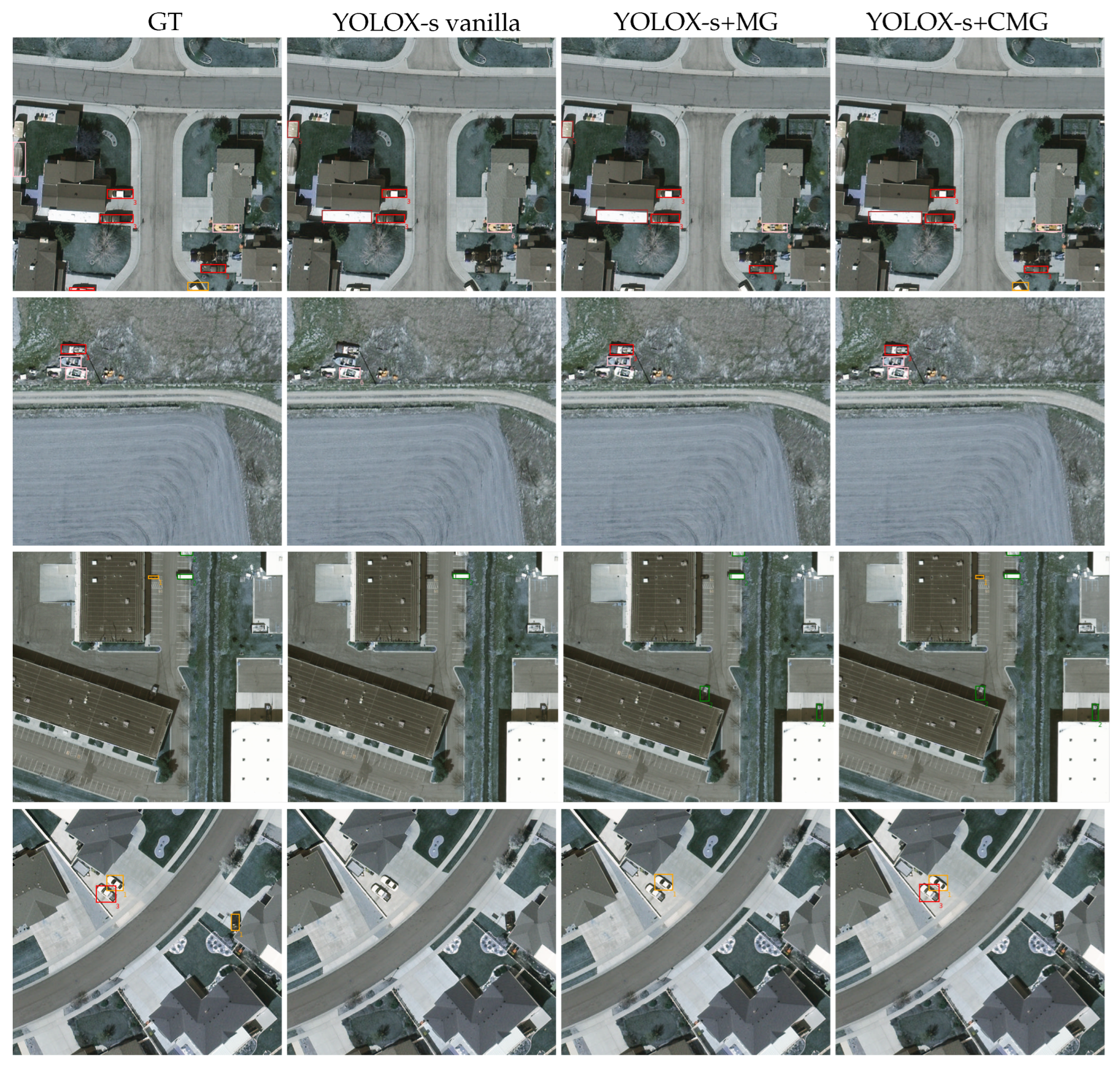
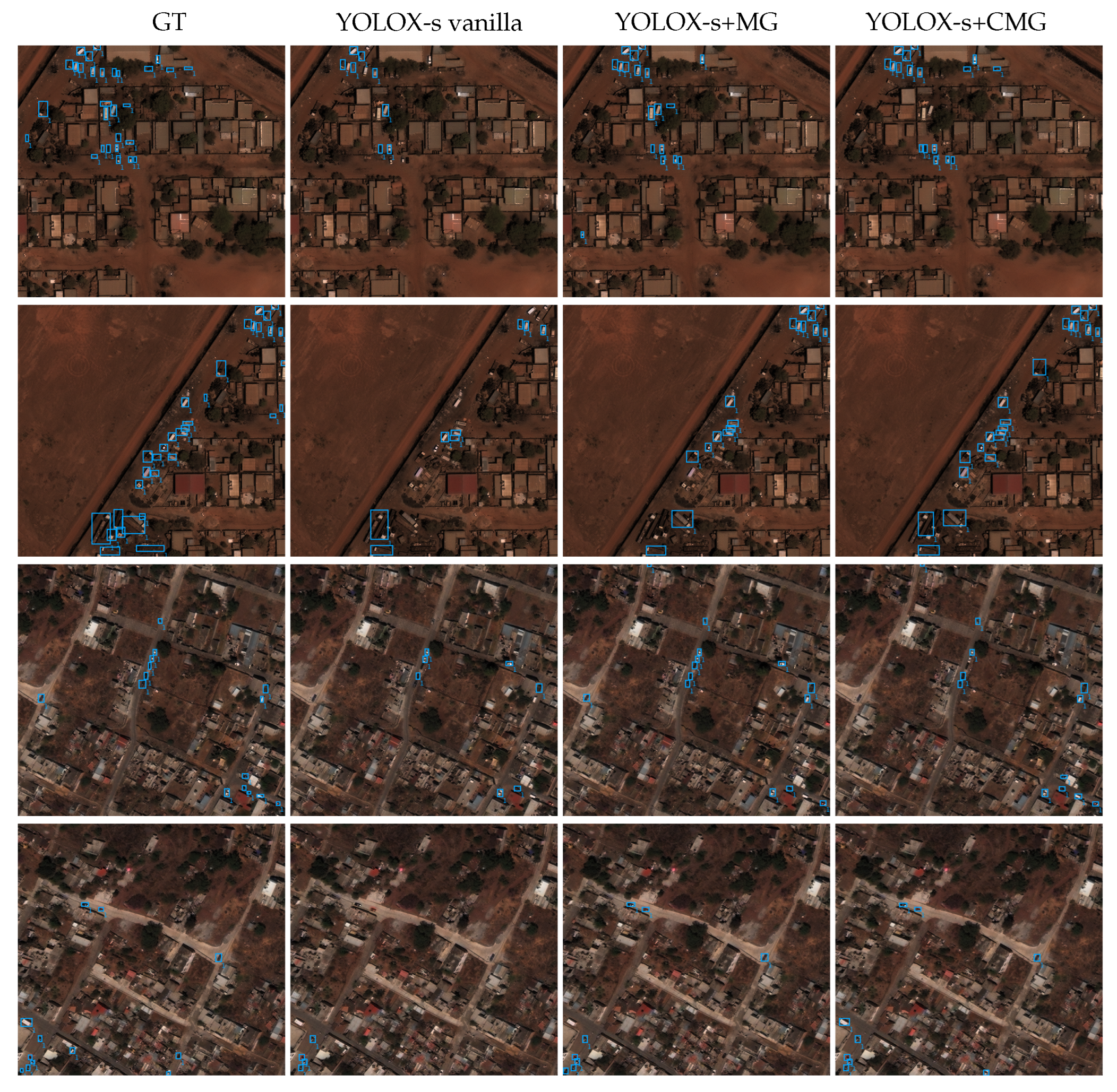
4.2. Mutual Guidance

In this section, we show the impact of mutual guidance on the remote sensing data by applying it directly for vehicle detection, apart from the other modules. The baseline is the same backbone with a generic setup, as used in [4]. As they use focal loss [45] in their setup, we include the mutual guidance with the same loss for a fair comparison.

The results in Table 1 show the improvement when switching from the IOU-based scheme to mutual guidance. The impact is diminished with YOLOX-m as was already efficient to begin with. The use of GFocal loss shows even further improvement for both architectures.

Table 1. Mutual guidance for different backbone architectures on VEDAI25 dataset. The best performance per column is shown in boldface.

Matching Strategy	Loss	YOLOX-s	YOLOX-m	YOLOv3
IOU-Based	Focal	70.20	74.30	70.78
Mutual Guidance	Focal	71.48	74.47	74.13
Mutual Guidance	GFocal	73.04	79.82	74.88

4.3. Contrastive Loss

Similar to the previous subsection, here, we aim to test the ability of contrastive loss in the context of vehicle detection. To this end, the contrastive loss is used together with the detection losses using the IOU-based matching strategy. Following [17], we also test the two possibilities of loss function, namely ${\mathcal{L}}_{\mathrm{in}}$ (Equation (7)) and ${\mathcal{L}}_{\mathrm{out}}$ (Equation (8)). The results are shown in Table 2.

Table 2. YOLOX-s performance on VEDAI25 with different contrastive loss functions.

Matching Strategy	Loss	YOLOX-s	YOLOX-m	YOLOv3
IOU-Based	Focal	70.20	74.30	70.78
	GFocal $+{\mathcal{L}}_{\mathrm{in}}$	71.53	79.89	75.53
	GFocal $+{\mathcal{L}}_{\mathrm{out}}$	74.20	77.81	74.41

The contrastive loss seems to have the reverse effect of mutual guidance on the two YOLOX backbones. The additional auxiliary loss does not improve the performance of YOLOX-s as highly as YOLOX-m, and, for the case of the outside loss, it even has negative impacts. This shows that YOLOX-m does not suffer from the misalignment problem as much as YOLOX-s does; thus, it can benefit more from the improvement in visual representation brought about by the contrastive loss.

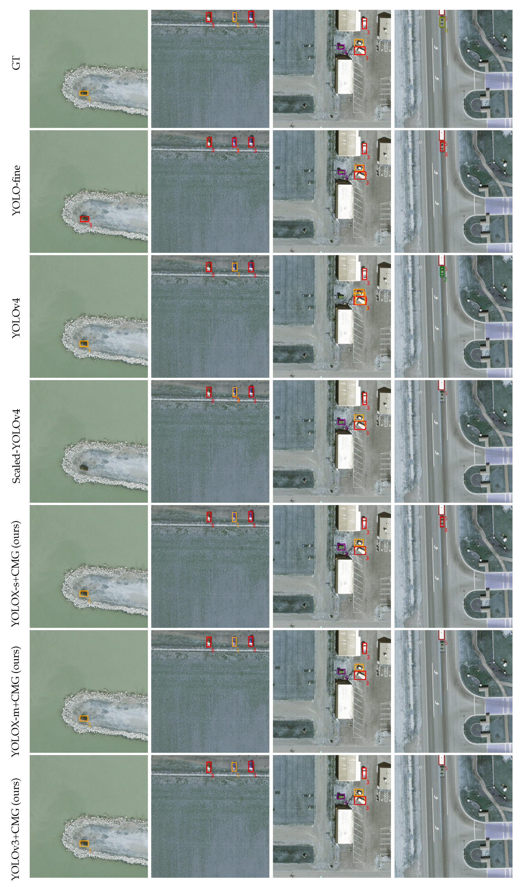
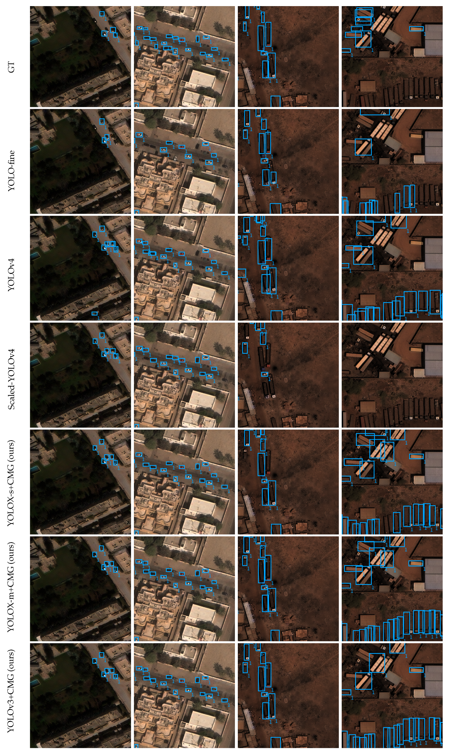
4.4. Mutual Guidance Meets Contrastive Learning

The results of YOLOX with the mutual guidance strategy and contrastive learning are shown in Table 3. Contrastive loss shows great benefit to the network when the misalignment between localization and classification is alleviated by mutual guidance. The improvement seems balanced between both backbones. Although the inside contrastive loss seems to dominate over the outside one in the previous experiment, it becomes inferior when the semantic information from the classification branch and projection head is properly utilized in the localization process, conforming to the finding from [17]. The combination of mutual guidance and outside contrastive loss is coined contrastive mutual guidance, or CMG.

Table 3. Performance of YOLOX backbones on VEDAI25 when training with mutual guidance (MG) and contrastive loss.

Matching Strategy	Loss	YOLOX-s	YOLOX-m	YOLOv3
Mutual Guidance	GFocal	73.04	79.82	74.88
	GFocal $+{\mathcal{L}}_{\mathrm{in}}$	75.57	80.95	76.26
	GFocal $+{\mathcal{L}}_{\mathrm{out}}$	76.67	81.57	77.41

Multiple datasets. We further show the results on different datasets with different resolutions in Table 4 and the corresponding precision-recall curve in Figure 4.

Table 4. Performance of YOLOX-s vanilla with mutual guidance (MG) and contrastive mutual guidance (CMG) on the 3 datasets. The contrastive mutual guidance strategy consistently out-performs other configurations, showing its benefit.

Configuration	VEDAI12	VEDAI25	xView30
vanilla	78.68	70.20	79.96
+MG	79.70	73.04	83.49
+CMG	81.25	76.67	83.67

Figure 4. Precision–recall curve of YOLOX-s on 3 datasets, from left to right: VEDAI12, VEDAI25, and xView30. The methods with +CMG gain improvement over the others at around recall level of 0.5 for the VEDAI datasets and both +MG and +CMG outperform the vanilla method on the xView dataset.

The methods with +CMG gain an improvement over the others at around a recall level of 0.5 for the VEDAI datasets and both +MG and +CMG outperform the vanilla method on the xView dataset.

Some qualitative results on the VEDAI25 and xView datasets can be found in Figure 5 and Figure 6, respectively. Several objects are missing in the second and third columns, while the CMG strategy (last column) is able to recognize objects of complex shape and appearance.

Figure 5. Qualitative results of YOLOX-s on VEDAI25. The contrastive mutual guidance helps to recognize intricate objects. The number and color of each box correspond to one of the classes, i.e., (1) car, (2) truck, (3) pickup, (4) tractor, (5) camper, (6) ship, (7) van, and (8) plane.

Figure 6. Qualitative results of YOLOX-s on xView. The contrastive mutual guidance helps to recognize intricate objects. The number and color of each box indicate the vehicle class.

Comparison to the state-of-the-art. In Table 5, we compare our method with several state-of-the-art methods on the three datasets. Our YOLOX backbone with the CMG strategy outperforms others on the VEDAI datasets and is on par with YOLO-fine on xView. From the qualitative results in Figure 7 and Figure 8, respectively, for the VEDAI and xView, it can be seen that although the xView dataset contains extremely small objects, our method, without deliberate operations for tiny object detection, can approach the state-of-the-art method specifically designed for small vehicle detection [28]. A breakdown of performance for each class of VEDAI is shown in Table 6.

Table 5. Performance of different YOLOX backbones with CMG compared to the state-of-the-art methods. Our method outperforms or is on par with the methods designed for tiny object recognition.

Architecture	VEDAI12	VEDAI25	xView30
EfficientDet	74.01	51.36	82.45
YOLOv3	73.11	62.09	78.93
YOLO-fine	76.00	68.18	84.14
YOLOv4	79.93	73.14	79.19
Scaled-YOLOv4	78.57	72.78	81.39
YOLOX-s+CMG (ours)	81.25	76.67	83.67
YOLOX-m+CMG (ours)	83.07	81.57	84.79
YOLOv3+CMG (ours)	78.09	77.41	83.54

Figure 7. Qualitative results of our methods and state-of-the-art methods on VEDAI25. The number and color of each box correspond to one of the classes, i.e. (1) car, (2) truck, (3) pickup, (4) tractor, (5) camper, (6) ship, (7) van, and (8) plane. The last column shows a failure case. Our method has difficulties in recognizing the “other” class, which comprises various object types.

Figure 8. Qualitative results of our methods and state-of-the-art methods on xView. The number and color of each box indicates the vehicle class. The last column shows a failure case. Our method could recognize objects of various shapes and would wrongly detect objects of extreme resemblance (although this might have been because of the faulty annotations).

Table 6. Per-class performance of YOLOX backbones with CMG on VEDAI25 dataset. Our method outperforms the state-of-the-art for all classes.

Model	Car	Truck	Pickup	Tractor	Camping	Boat	Van	Other	mAP
EfficientDet	69.08	61.20	65.74	47.18	69.08	33.65	16.55	36.67	51.36
YOLOv3	75.22	73.53	65.69	57.02	59.27	47.20	71.55	47.20	62.09
YOLOv3-tiny	64.11	41.21	48.38	30.04	42.37	24.64	68.25	40.77	44.97
YOLOv3-spp	79.03	68.57	72.30	61.67	63.41	44.26	60.68	42.43	61.57
YOLO-fine	76.77	63.45	74.35	78.12	64.74	70.04	77.91	45.04	68.18
YOLOv4	87.50	80.47	78.63	65.80	81.07	75.92	66.56	49.16	73.14
Scaled-YOLOv4	86.78	79.37	81.54	73.83	71.58	76.53	63.90	48.70	72.78
YOLOX-s+CMG (ours)	88.92	85.92	79.66	77.16	81.21	65.22	64.90	70.33	76.67
YOLOX-m+CMG (ours)	91.26	85.34	84.91	76.22	85.03	78.68	82.02	69.08	81.57
YOLOv3 +CMG (ours)	92.20	85.98	87.34	77.27	85.56	53.74	73.94	64.13	77.41

Two failure cases are shown in the last columns of Figure 7 and Figure 8. We can see that our method has difficulty in recognizing the “other” class (VEDAI), which comprises various object types, and might wrongly detect objects of extreme resemblance (xView).

5. Discussion

Although supervised contrastive loss has been shown to be able to replace cross-entropy for classification problems [17], in this paper, contrastive loss is applied as an auxiliary loss besides the main localization and classification losses. This is because only a small number of anchors are involved in the contrastive process due to the large number of anchors, especially negative anchors.

However, contrastive loss shows weakness when the annotations are noisy, such as those of the xView dataset. Several boxes are missing for (what appear to be) legitimate objects, as shown in Figure 9.

Figure 9. Examples of faulty annotations in the xView dataset: non-vehicle annotation (red border), missing annotations of container trucks (green border), and cars (blue border). The number and color of each box indicates the vehicle class.

It is shown from the experimental results that inward contrastive loss is not always inferior to its outward counterpart, as shown in [17]. We speculate that this could be due to the auxiliary role of contrastive loss in the detection problem and/or the characteristics of small objects in remote sensing images.

6. Conclusions

This paper presents a combination of a mutual guidance matching strategy and supervised contrastive loss for the vehicle detection problem. The mutual guidance helps in better connecting the localization and classification branches of a detection network, while contrastive loss improves the visual representation, which provides better semantic information. The vehicle detection task is generally complicated due to the varied object sizes and similar appearances from the aerial point of view. This, however, provides an opportunity for contrastive learning, as it can be regarded as image augmentation, which has been shown to be beneficial for learning visual representations. Although the paper is presented in a remote sensing context, we believe that this idea could be expanded to generic computer vision applications.

References

1. Wu, Y.; Chen, Y.; Yuan, L.; Liu, Z.; Wang, L.; Li, H.; Fu, Y. Rethinking Classification and Localization for Object Detection. In Proceedings of the IEEE/CVF Conference on Computer Vision and Pattern Recognition (CVPR), Seattle, WA, USA, 13–19 June 2020. [Google Scholar]
2. Jiang, B.; Luo, R.; Mao, J.; Xiao, T.; Jiang, Y. Acquisition of Localization Confidence for Accurate Object Detection. In Proceedings of the European Conference on Computer Vision (ECCV), Munich, Germany, 8–14 September 2018. [Google Scholar]
3. Song, G.; Liu, Y.; Wang, X. Revisiting the Sibling Head in Object Detector. In Proceedings of the IEEE/CVF Conference on Computer Vision and Pattern Recognition (CVPR), Seattle, WA, USA, 13–19 June 2020. [Google Scholar]
4. Zhang, H.; Fromont, E.; Lefevre, S.; Avignon, B. Localize to Classify and Classify to Localize: Mutual Guidance in Object Detection. In Proceedings of the Asian Conference on Computer Vision (ACCV), Online, 30 November–4 December 2020. [Google Scholar]
5. Kaack, L.H.; Chen, G.H.; Morgan, M.G. Truck Traffic Monitoring with Satellite Images. In Proceedings of the ACM SIGCAS Conference on Computing and Sustainable Societies, Accra, Ghana, 3–5 July 2019. [Google Scholar]
6. Arora, N.; Kumar, Y.; Karkra, R.; Kumar, M. Automatic vehicle detection system in different environment conditions using fast R-CNN. Multimed. Tools Appl. 2022, 81, 18715–18735. [Google Scholar] [CrossRef]
7. Zhou, H.; Creighton, D.; Wei, L.; Gao, D.Y.; Nahavandi, S. Video Driven Traffic Modelling. In Proceedings of the IEEE/ASME International Conference on Advanced Intelligent Mechatronics, Wollongong, NSW, Australia, 9–12 July 2013. [Google Scholar]
8. Kamenetsky, D.; Sherrah, J. Aerial Car Detection and Urban Understanding. In Proceedings of the International Conference on Digital Image Computing: Techniques and Applications (DICTA), Adelaide, SA, Australia, 23–25 November 2015. [Google Scholar]
9. Shi, F.; Zhang, T.; Zhang, T. Orientation-Aware Vehicle Detection in Aerial Images via an Anchor-Free Object Detection Approach. IEEE Trans. Geosci. Remote. Sens. 2021, 59, 5221–5233. [Google Scholar] [CrossRef]
10. Zheng, K.; Wei, M.; Sun, G.; Anas, B.; Li, Y. Using Vehicle Synthesis Generative Adversarial Networks to Improve Vehicle Detection in Remote Sensing Images. ISPRS Int. J. -Geo-Inf. 2019, 8, 390. [Google Scholar] [CrossRef] [Green Version]
11. Bouguettaya, A.; Zarzour, H.; Kechida, A.; Taberkit, A.M. Vehicle Detection From UAV Imagery With Deep Learning: A Review. IEEE Trans. Neural Netw. Learn. Syst. 2021. [Google Scholar] [CrossRef] [PubMed]
12. Lin, T.Y.; Maire, M.; Belongie, S.; Hays, J.; Perona, P.; Ramanan, D.; Dollar, P.; Zitnick, C.L. Microsoft COCO: Common Objects in Context. In Proceedings of the European Conference on Computer Vision (ECCV), Zurich, Switzerland, 6–12 September 2014. [Google Scholar]
13. Everingham, M.; Van Gool, L.; Williams, C.K.I.; Winn, J.; Zisserman, A. The Pascal Visual Object Classes (VOC) Challenge. Int. J. Comput. Vis. 2010, 88, 303–338. [Google Scholar] [CrossRef] [Green Version]
14. Bachman, P.; Hjelm, R.D.; Buchwalter, W. Learning Representations by Maximizing Mutual Information across Views. In Proceedings of the 33rd International Conference on Neural Information Processing Systems, Vancouver, BC, Canada, 8–14 December 2019. [Google Scholar]
15. Dosovitskiy, A.; Springenberg, J.T.; Riedmiller, M.; Brox, T. Discriminative Unsupervised Feature Learning with Convolutional Neural Networks. In Proceedings of the Advances in Neural Information Processing Systems, Montreal, QC, Canada, 8–13 December 2014. [Google Scholar]
16. Chen, T.; Kornblith, S.; Norouzi, M.; Hinton, G. A Simple Framework for Contrastive Learning of Visual Representations. In Proceedings of the ICML, 2020, Machine Learning Research, Vienna, Austria, 13–18 July 2020. [Google Scholar]
17. Khosla, P.; Teterwak, P.; Wang, C.; Sarna, A.; Tian, Y.; Isola, P.; Maschinot, A.; Liu, C.; Krishnan, D. Supervised Contrastive Learning. In Proceedings of the Advances in Neural Information Processing Systems, Virtual, 6–12 December 2020. [Google Scholar]
18. Wei, F.; Gao, Y.; Wu, Z.; Hu, H.; Lin, S. Aligning Pretraining for Detection via Object-Level Contrastive Learning. In Proceedings of the Advances in Neural Information Processing Systems, Virtual, 6–14 December 2021. [Google Scholar]
19. Xie, E.; Ding, J.; Wang, W.; Zhan, X.; Xu, H.; Sun, P.; Li, Z.; Luo, P. DetCo: Unsupervised Contrastive Learning for Object Detection. In Proceedings of the IEEE/CVF International Conference on Computer Vision (ICCV), Montreal, QC, Canada, 10–17 October 2021. [Google Scholar]
20. Xie, Z.; Lin, Y.; Zhang, Z.; Cao, Y.; Lin, S.; Hu, H. Propagate Yourself: Exploring Pixel-Level Consistency for Unsupervised Visual Representation Learning. In Proceedings of the IEEE/CVF Conference on Computer Vision and Pattern Recognition (CVPR), Nashville, TN, USA, 20–25 June 2021. [Google Scholar]
21. Razakarivony, S.; Jurie, F. Vehicle detection in aerial imagery: A small target detection benchmark. J. Vis. Commun. Image Represent. 2016, 34, 187–203. [Google Scholar] [CrossRef] [Green Version]
22. Lam, D.; Kuzma, R.; McGee, K.; Dooley, S.; Laielli, M.; Klaric, M.; Bulatov, Y.; McCord, B. xView: Objects in Context in Overhead Imagery. arXiv 2018, arXiv:1802.07856. [Google Scholar]
23. Froidevaux, A.; Julier, A.; Lifschitz, A.; Pham, M.T.; Dambreville, R.; Lefèvre, S.; Lassalle, P. Vehicle detection and counting from VHR satellite images: Efforts and open issues. In Proceedings of the IGARSS 2020-2020 IEEE International Geoscience and Remote Sensing Symposium, Waikoloa, HI, USA, 26 September–2 October 2020. [Google Scholar]
24. Srivastava, S.; Narayan, S.; Mittal, S. A survey of deep learning techniques for vehicle detection from UAV images. J. Syst. Archit. 2021, 117, 102152. [Google Scholar] [CrossRef]
25. Zou, Z.; Shi, Z.; Guo, Y.; Ye, J. Object detection in 20 years: A survey. arXiv 2019, arXiv:1905.05055. [Google Scholar]
26. Ji, H.; Gao, Z.; Mei, T.; Li, Y. Improved faster R-CNN with multiscale feature fusion and homography augmentation for vehicle detection in remote sensing images. IEEE Geosci. Remote. Sens. Lett. 2019, 16, 1761–1765. [Google Scholar] [CrossRef]
27. Mo, N.; Yan, L. Improved faster RCNN based on feature amplification and oversampling data augmentation for oriented vehicle detection in aerial images. Remote. Sens. 2020, 12, 2558. [Google Scholar] [CrossRef]
28. Pham, M.T.; Courtrai, L.; Friguet, C.; Lefèvre, S.; Baussard, A. YOLO-Fine: One-Stage Detector of Small Objects Under Various Backgrounds in Remote Sensing Images. Remote. Sens. 2020, 12, 2501. [Google Scholar] [CrossRef]
29. Koay, H.V.; Chuah, J.H.; Chow, C.O.; Chang, Y.L.; Yong, K.K. YOLO-RTUAV: Towards Real-Time Vehicle Detection through Aerial Images with Low-Cost Edge Devices. Remote Sens. 2021, 13, 4196. [Google Scholar] [CrossRef]
30. Guo, Y.; Xu, Y.; Li, S. Dense construction vehicle detection based on orientation-aware feature fusion convolutional neural network. Autom. Constr. 2020, 112, 103124. [Google Scholar] [CrossRef]
31. Yang, J.; Xie, X.; Shi, G.; Yang, W. A feature-enhanced anchor-free network for UAV vehicle detection. Remote. Sens. 2020, 12, 2729. [Google Scholar] [CrossRef]
32. Li, Y.; Pei, X.; Huang, Q.; Jiao, L.; Shang, R.; Marturi, N. Anchor-free single stage detector in remote sensing images based on multiscale dense path aggregation feature pyramid network. IEEE Access 2020, 8, 63121–63133. [Google Scholar] [CrossRef]
33. Tseng, W.H.; Lê, H.Â.; Boulch, A.; Lefèvre, S.; Tiede, D. CroCo: Cross-Modal Contrastive Learning for Localization of Earth Observation Data. In Proceedings of the ISPRS Annals of the Photogrammetry, Remote Sensing and Spatial Information Sciences, Nice, France, 6–11 June 2022. [Google Scholar]
34. Sohn, K. Improved Deep Metric Learning with Multi-class N-pair Loss Objective. In Proceedings of the Advances in Neural Information Processing Systems, Barcelona, Spain, 5–10 December 2016. [Google Scholar]
35. Weinberger, K.Q.; Blitzer, J.; Saul, L. Distance Metric Learning for Large Margin Nearest Neighbor Classification. In Proceedings of the Advances in Neural Information Processing Systems, Vancouver, BC, Canada, 5–8 December 2005. [Google Scholar]
36. Wang, X.; Zhang, R.; Shen, C.; Kong, T.; Li, L. Dense Contrastive Learning for Self-Supervised Visual Pre-Training. In Proceedings of the IEEE/CVF Conference on Computer Vision and Pattern Recognition (CVPR), Nashville, TN, USA, 20–25 June 2021. [Google Scholar]
37. Lin, T.Y.; Dollar, P.; Girshick, R.; He, K.; Hariharan, B.; Belongie, S. Feature Pyramid Networks for Object Detection. In Proceedings of the IEEE Conference on Computer Vision and Pattern Recognition (CVPR), Honolulu, HI, USA, 21–26 July 2017. [Google Scholar]
38. Redmon, J.; Farhadi, A. Yolov3: An incremental improvement. arXiv 2018, arXiv:1804.02767. [Google Scholar]
39. Jaccard, P. The distribution of the Flora in the Alpine Zone. 1. New Phytol. 1912, 11, 37–50. [Google Scholar] [CrossRef]
40. Li, X.; Wang, W.; Wu, L.; Chen, S.; Hu, X.; Li, J.; Tang, J.; Yang, J. Generalized Focal Loss: Learning Qualified and Distributed Bounding Boxes for Dense Object Detection. In Proceedings of the Advances in Neural Information Processing Systems, Online, 6–12 December 2020. [Google Scholar]
41. Pang, J.; Chen, K.; Shi, J.; Feng, H.; Ouyang, W.; Lin, D. Libra R-CNN: Towards Balanced Learning for Object Detection. In Proceedings of the IEEE Conference on Computer Vision and Pattern Recognition, Long Beach, CA, USA, 16–20 June 2019. [Google Scholar]
42. Ge, Z.; Liu, S.; Wang, F.; Li, Z.; Sun, J. YOLOX: Exceeding YOLO Series in 2021. arXiv 2021, arXiv:2107.08430. [Google Scholar]
43. Tan, M.; Pang, R.; Le, Q.V. Efficientdet: Scalable and efficient object detection. In Proceedings of the IEEE/CVF Conference on Computer Vision and Pattern Recognition, Seattle, WA, USA, 13–19 June 2020. [Google Scholar]
44. Wang, C.Y.; Bochkovskiy, A.; Liao, H.Y.M. Scaled-yolov4: Scaling cross stage partial network. In Proceedings of the IEEE/CVF Conference on Computer Vision and Pattern Recognition, Nashville, TN, USA, 20–25 June 2021. [Google Scholar]
45. Lin, T.Y.; Goyal, P.; Girshick, R.; He, K.; Dollar, P. Focal Loss for Dense Object Detection. In Proceedings of the IEEE International Conference on Computer Vision (ICCV), Venice, Italy, 22–29 October 2017. [Google Scholar]
Publisher’s Note: MDPI stays neutral with regard to jurisdictional claims in published maps and institutional affiliations.
Article Metrics
Citations
Article Access Statistics
Multiple requests from the same IP address are counted as one view.