A Fast and Precise Plane Segmentation Framework for Indoor Point Clouds

Abstract

To improve the efficiency and accuracy of plane segmentation for indoor point clouds, this paper proposes a fast and precise plane segmentation framework which mainly consists of two steps: plane rough segmentation and precise segmentation. In the rough segmentation stage, the point clouds are firstly voxelized, then the original plane is extracted roughly according to the plane normal vector and nearest voxels conditions. Based on the results of rough segmentation, a further operation composed of downsampling and density-based spatial clustering of applications with noise (DBSCAN) is adopted to produce efficient and precise segmentation. Finally, to correct the over-segmentation, the distance and normal vector angle thresholds between planes are taken into consideration. The experimental results show that the proposed method improves the efficiency and accuracy of indoor point cloud plane segmentation, and the average intersection-over-union (IoU) achieves 0.8653.

1. Introduction

Accurate and economical LiDAR can be used to intuitively create a complete 3D model of the real world [1,2], which makes LiDAR widely applied to autonomous driving [3,4,5], simultaneous localization and mapping (SLAM) [6,7,8], 3D reconstruction [9,10,11,12,13] and other fields. For the task of 3D reconstruction, plane extraction is crucial, and a lot of research has been proposed to address the plane extraction issue.

Due to the disorder and high density of point clouds, the direct plane segmentation algorithms are time-consuming and tend to generate under-segmentation or over-segmentation results. To solve this problem, there are several ideas for extracting plane point clouds: region growing [14,15,16], random sample consensus (RANSAC) [17,18], normal estimation [19,20], dimensionality reduction algorithms [21,22], and density-based noise application spatial clustering [23,24]. The region growing methods have high accuracy, stability, and robustness [25]. The seed points are selected by the constraints of height, curvature, and the number of neighbor points. The seed growing conditions are determined according to the angle threshold of the tangent plane of the seed points. Su et al. [26] combined a region growing algorithm and distance algorithm to extract planes precisely. Dong et al. [27] observed global information and enriched the results from region growing with global energy optimization. RANSAC is generally used in combination with other methods [28,29] to generate precise results. Yuan et al. [30] adopted RANSAC to first roughly segment the point cloud, then used the region growing algorithm to optimize the plane. To improve the accuracy of RANSAC segmentation, Xu et al. [31] proposed a point cloud pre-classification method based on support vector machine classification. The method based on the region growing algorithm or RANSAC can yield results with high accuracy, but it will be inefficient with the increasing scale of the data as well. To weaken the influence of the scale of data and improve the efficiency, normal estimations are taken into consideration. Yang et al. [32] first used the weighted PCA method to estimate the point cloud normal vector, then used angle clustering to obtain a series of parallel planes. Finally, the improved RANSAC was used to detect the horizontal distance and normal distance between planes, respectively, extracting the adjacent overlapping planes in space. Moreover, voxelization [33,34] is also an important means to improve computational efficiency. Huang et al. [35] proposed an efficient encoding voxel-based segmentation (EVBS) algorithm based on fast adjacent voxel search, which can segment point cloud planes faster and more accurately than traditional algorithms. Xu et al. [36] also used the voxelized structure of the point cloud combined with the face-based global clustering to automatically extract planes in an unsupervised way. Lee [37], Saglam [38], and Vo [39] also proceeded to the next steps after voxelizing the point cloud in the preprocessing stage. Voxelization can give the point cloud a topological structure, thereby the improving computational efficiency. However, high efficiency and high accuracy are often difficult to be satisfy simultaneously. Therefore, some additional methods are needed to improve the segmentation accuracy. The point cloud on the same plane has the characteristics of being uniform, continuous, and high-density, and the DBSCAN clustering algorithm can classify the points of continuous and uniform density to achieve the accurate segmentation of the plane. Czerniawski et al. [40] proposed combining the semantic information stored in the plane in which the DBSCAN was used in the 6D space, and trained a decision tree classifier through dimensionality reduction and unsupervised learning, which can achieve more than 90% accuracy in large-scale building plane segmentation (walls, ground, and ceiling). Based on candidate sample selection and plane validity detection in 3D space, Chen et al. [41] proposed additional DBSCAN clustering conditions and adaptive thresholds to obtain effective fitting planes. Although DBSCAN has a good segmentation performance, the parameters of the algorithm cannot be explicitly determined, and additional determination conditions need to be set. Meanwhile, when the scale of the point cloud is large, the algorithm will be time-consuming. As mentioned above, how to quickly and accurately segment plane point clouds is still a difficult problem in 3D point cloud processing.

To solve this problem, we considered using voxelization to improve the computational efficiency and adopting clustering methods to make up for the lack of segmentation accuracy. First, the point cloud voxelization makes the disordered point cloud be arranged regularly; each point corresponds to a unique voxel, and the corresponding voxel can be quickly accessed by number. In addition, the points in each voxel can be regarded as a whole, and the normal vector, curvature, and the number of points fitted with these points can be used as the characteristics of each voxel. With voxelization, each plane consists of multiple voxels, and the points in each voxel can be fitted a local normal vector. Therefore, the plane can quickly be determined by the normal vector, avoiding the time-consuming calculation of the normal vector of each point. Through some verified experiments, we adopted the DBSCAN algorithm to achieve further segmentation. Although this method can achieve fine segmentation to improve accuracy, we found that when the number of points in a cloud is in the hundreds of thousands or even millions, the method can take hours or even days to complete the segmentation. Furthermore, the two parameters of the radius and the number of points within the radius are difficult to determine in this algorithm, it needs to be continuously adjusted to the optimal parameters to have a better effect. Therefore, we proposed a framework combining the advantages of voxelization and DBSCAN to quickly and precisely realize the segmentation of planes. The overall flow of the framework in this paper is shown in Figure 1.

The organization of this paper can be summarized as follows: In Section 2, we elaborate on the principle of the proposed algorithm in three steps. Section 2.1 introduces the plane rough segmentation based on nearest-neighbor voxels; Section 2.2 presents the plane precise segmentation based on DBSCAN; the post-processing and optimization of the algorithm are introduced in Section 2.3. Section 3.1 describes the equipment we use, the measurement principle of this equipment, and how we obtain raw data; Section 3.2 illustrates the algorithm with three different scenarios; Section 3.3 calculates the experimental parameters, and evaluates the method proposed in this paper by comparing it with other methods. In Section 4, the experimental results are objectively analyzed and discussed, illustrating the strengths and weaknesses of our method. Finally, we summarize the full work of this paper and future work directions in Section 5.

2. Methods

The 3D point cloud segmentation algorithm will be introduced in this section in three stages: (1) the plane rough segmentation based on the nearest-neighbor voxel; (2) precise segmentation for rough planes obtained in (1) based on DBSCAN; and (3) optimization to mitigate the over-segmentation phenomenon.

2.1. Plane Rough Segmentation Based on Voxels

The rough plane extraction algorithm is divided into two steps: The raw point clouds are voxelized, and the local normal vector characteristics of the nearest-neighbor voxels are used to achieve the preliminary plane extraction. As shown in Figure 2, it is a flowchart of the algorithm for the rough segmentation of the raw point clouds.

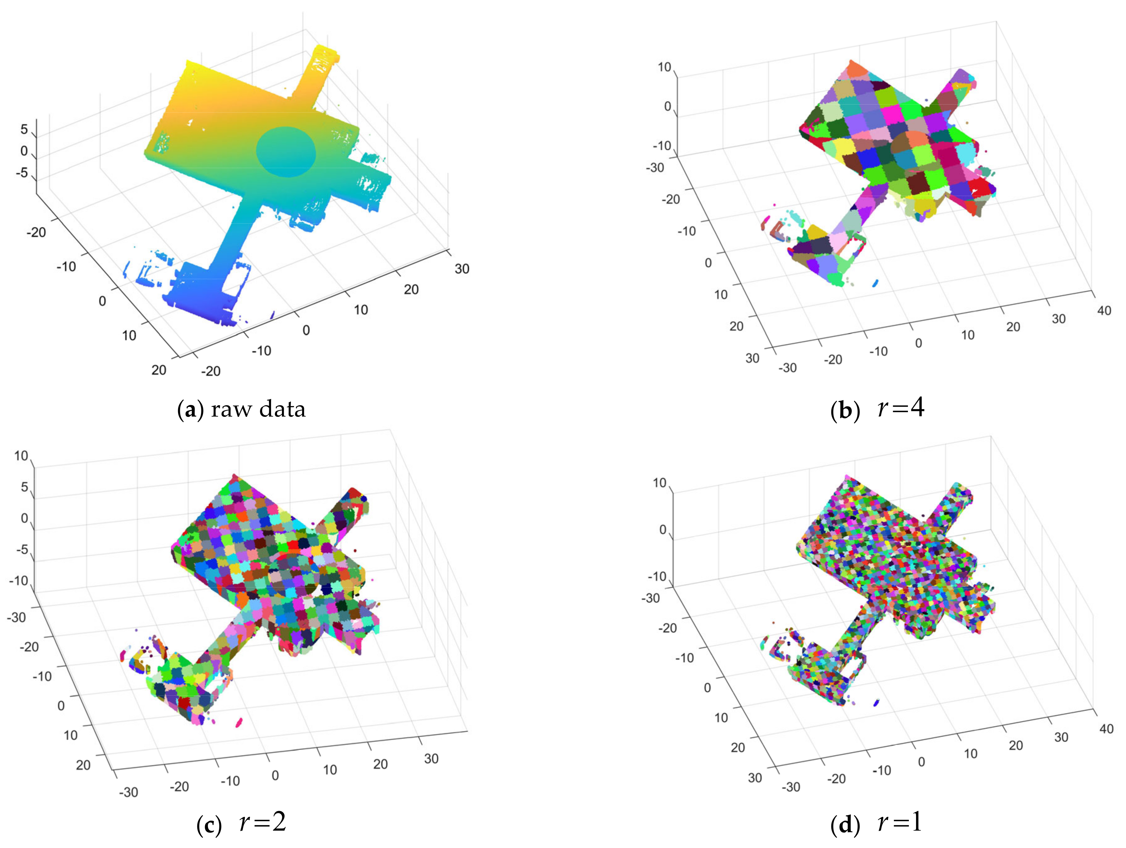
For the raw point clouds, $x_{\min },x_{\max },y_{\min },\cdots ,z_{\max }$ (the maximum and minimum values of the point cloud in the three directions, $x,y,z$) are easily obtained. Then, the number of voxel grids in each direction could be determined by relying on a given voxel size. (It is assumed here that the voxel sizes in the three directions are all $r$. In practical applications, different sizes can be selected according to needs.) The voxel segmentation results of different sizes are shown in Figure 3. Therefore, the voxel number $\left(x_i,y_i,z_i\right)$ in three directions corresponding to each point is:

$$\left\{\begin{array}{l}{N}_x=\left(x_{\max }-x_{\min }\right)/r\\ N_y=\left(y_{\max }-y_{\min }\right)/r\\ N_z=\left(z_{\max }-z_{\min }\right)/r\end{array}\right.$$

(1)

$$\left\{\begin{array}{cc}\begin{array}{l}{x}_i=\frac{\left(x-x_{\min }\right)}{r}=a,\\ y_i=\frac{\left(y-y_{\min }\right)}{r}=b,\\ z_i=\frac{\left(z-z_{\min }\right)}{r}=c,\end{array}& (i=1,2,\cdots ,n)\end{array}\right.$$

(2)

Then, we store all points in a voxel structure as follows:

$$P_r=\left\{G\left|G=g\left(a,b,c\right),a=1,2,\cdots ,N_x;b=1,2,\cdots ,N_y;c=1,2,\cdots ,N_z;\right.\right\}$$

(3)

where $g\left(a,b,c\right)$ represents the voxels numbered $\left(a,b,c\right)$. The raw point cloud is converted into the voxel structure of $N_x\times N_y\times N_z$; hence, each point has a corresponding voxel number, and the corresponding point can be accessed according to the number. Next, all the voxels are traversed in turn. For the seed voxel $g\left(a,b,c\right)$, the points in the voxels are:

$$g\left(a,b,c\right)=\left[g_1,g_2,\cdots ,g_k\right]$$

(4)

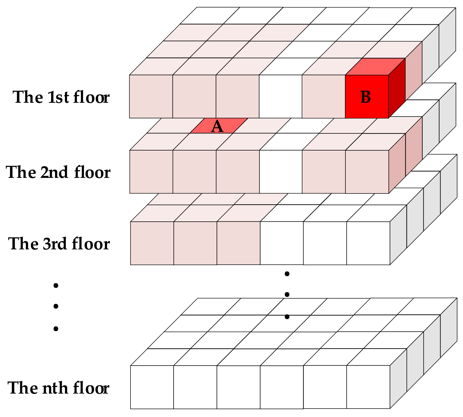
where $g_1,g_2,\cdots ,g_k$ are the points in $g\left(a,b,c\right)$. Afterward, we find a plane mapped via principal component analysis (PCA) with the points in the voxel and obtain the eigenvector $v_0$ corresponding to the smallest eigenvalue as the normal vector of the plane. The same operation is performed on the adjacent 26 voxels surrounding the voxel, where edge constraints are required; that is, the maximum number of nearest-neighbor voxels is 26 and the minimum is 7, and the two distributions are shown in Figure 4.

It should be pointed out that the orientation of voxelization is not always parallel or perpendicular to the plane in the point cloud because of the orientation difference between the different point clouds. However, when there is a plane intersecting with the seed voxel, the number of nearest-neighbor voxels intersecting with the plane is at least $k\left(k\ge 8\right)$. Therefore, it can be determined whether the currently traversed seed voxel is the target voxel according to $k$. At the same time, a threshold ${\sigma }_1$ is set to remove the voxels with a few points in the calculation to weaken the influence of noise.

When $k=8$ and the target plane is parallel to the voxel obtained above, the voxels to be calculated are:

$$\Im =\left[\begin{array}{ccc}g\left(a-1,b,c-1\right)& g\left(a-1,b,c\right)& g\left(a-1,b,c+1\right)\\ g\left(a,b,c-1\right)& g\left(a,b,c\right)& g\left(a,b,c+1\right)\\ g\left(a+1,b,c-1\right)& g\left(a+1,b,c\right)& g\left(a+1,b,c+1\right)\end{array}\right]$$

(5)

and the local normal vectors of each voxel are:

$$\aleph =\left[\begin{array}{ccc}{v}_1& v_2& v_3\\ v_4& v_0& v_5\\ v_6& v_7& v_9\end{array}\right]$$

(6)

Therefore, the angles between the central normal vector $v_0$ and the adjacent 8 normal vectors are:

$$\mathsf{\Phi }=\left[\begin{array}{ccc}{\theta }_1& {\theta }_2& {\theta }_3\\ {\theta }_4& 0& {\theta }_5\\ {\theta }_6& {\theta }_7& {\theta }_8\end{array}\right]$$

(7)

Setting an angle threshold ${\theta }_0$, when all the angles in $\mathsf{\Phi }$ satisfy the condition of Formula (8), the central voxel and the adjacent 8 voxels are considered to be part of the plane. Otherwise, it will traverse the remaining voxels until the next voxel that satisfies the condition is found. The current algorithm stops as soon as all voxels have been traversed or all planes have been found.

$${\theta }_i<{\theta }_0,\left(i=1,2,\cdots ,8\right)$$

(8)

When a plane is determined, all the points in the seed voxels and the adjacent 8 voxels are:

$${\mathrm{\Xi }}_i^{\prime }=\left(g_1,g_2,\cdots ,g_m\right)$$

(9)

Next, the least-squares method is used to perform plane fitting on all points contained in ${\mathrm{\Xi }}_i^{\prime }$, and the obtained fitting plane ${\mathrm{\Xi }}_i^{″}$ is:

$$A_{i}x+B_{i}y+C_{i}z+D_i=0$$

(10)

Afterward, the distances between all points and the plane are calculated, and if the distance is less than the threshold $\lambda$, all corresponding points are regarded as the preliminary point of the plane:

$$\frac{\left|A_i{x}_j+B_i{y}_j+C_i{z}_j+D_i\right|}{\sqrt{A_i^2+B_i^2+C_i^2}}<\lambda ,j=1,2,\cdots ,m$$

(11)

Here, the plane ${\mathrm{\Xi }}_i$ of the raw data is obtained. Then, we delete the currently found plane points in the original data, take the remaining data as the new initial data and repeat the above operations until all the planes are found. We stipulate that if there are no voxels meeting the condition again or the number of remaining points is less than the threshold after traversing all voxels, the loop operation is interrupted. The single-pass plane determination process of the normal vector is shown in Figure 5.

In this step, slices of each plane are obtained, but these slices have the characteristic of infinite size; that is, they contain both plane points and sparse points elsewhere, and this problem will be solved in the next subsection. The pseudo-code of rough segmentation based on voxels is shown in Algorithm 1.

Algorithm 1 Plane rough segmentation based on voxels

Input:$P_0(n\times 3points)$ Output: ${\mathrm{\Xi }}_1,{\mathrm{\Xi }}_2,\cdots ,{\mathrm{\Xi }}_i$ 1: for$P_0$ do 2:   $voxelization\leftarrow P_0$ 3:   for $g\left(a,b,c\right)\in P_r$ do 4:     $v_i\leftarrow g\left(a,b,c\right)$ do PCA 5:     ${\theta }_i\leftarrow \angle \left[v_0,v_i\right]\left(i=1,2,\dots ,8\right)$ 6:     if ${\theta }_i<{\theta }_0$ do 7:       ${\mathrm{\Xi }}_i^{″}\leftarrow {\mathrm{\Xi }}_i^{\prime }$ do PCA 8:       ${\mathrm{\Xi }}_i\leftarrow g=\left\{g\left|g=g_j,dis\left(g_j\in P_r,{\mathrm{\Xi }}_i\right)<\lambda \right.\right\}$ 9:       break 10:     end if 11:   end for 12:   ${\mathrm{\Xi }}_1,{\mathrm{\Xi }}_2,\dots ,{\mathrm{\Xi }}_i$ 13: end for

2.2. Precise Segmentation of Plane Based on DBSCAN

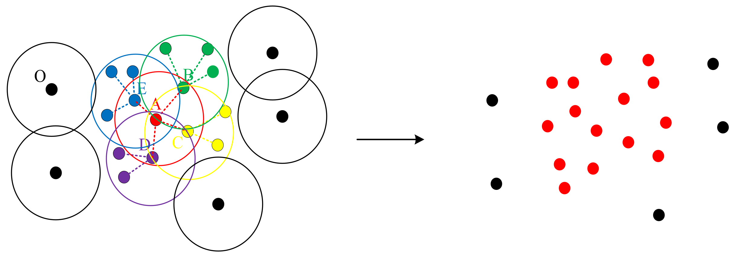
The DBCSAN is a traditional clustering algorithm that can classify high-density point clouds into one category according to the density of the points. The basic idea of the algorithm is shown in Figure 6. To begin with, the initial core density point $A$ is randomly determined, and the radius $R$ and the number $N$ of points within the radius of $A$ are artificially defined. If the number of points within the radius of $A$ is greater than $N$, the point will be taken as the initial core density point and all the points contained in the radius are also considered as new core density points. Then, the operation to find new core density points is repeated again and again until the points in the radius of all the core density points do not meet the density condition. Finally, we take all the core density points and all the points within the radius of the core density point as one category and the others as outliers. After the first category is determined, an initial core density point is randomly selected and the above steps are repeated again until all points have been visited, and the algorithm stops.

DBSCAN is an unsupervised clustering algorithm that can autonomously find several possible high-density point clusters in the data. In the experiment, we find that the category obtained via DBSCAN from the plane in rough segmentation is the exact plane that we expect. However, the shortcomings of DBSCAN are obvious as well. With the growth in the scale or dimension of the data, the time consumption increases while the efficiency decreases. Therefore, we propose a precise segmentation algorithm based on DBSCAN, which means that the time consumption of precise segmentation does not change significantly with the increasing scale of the data. The algorithm process is shown in Figure 7.

The mathematical representation of the mapping plane ${\mathrm{\Xi }}_i$ obtained in Section 2.1 is as follows:

$$A_{i}x+B_{i}y+C_{i}z+D_i=0,(i=1,2,\cdots ,m)$$

(12)

where the normal vector of ${\mathrm{\Xi }}_i$ is $\nu =\left[A_i,B_i,C_i\right]$ and the two normal vectors that are perpendicular to $\nu$ and perpendicular with each other are acquired via PCA:

$$\left[{\nu }_1,{\nu }_2\right]=\left[\begin{array}{l}\begin{array}{cc}{a}_1& a_2\end{array}\\ \begin{array}{cc}{b}_1& b_2\end{array}\\ \begin{array}{cc}{c}_1& c_2\end{array}\end{array}\right]$$

(13)

Then, the three-dimensional plane ${\mathrm{\Xi }}_i$ can be projected to a two-dimensional plane:

$${\mathrm{\Xi }}_i^2={\mathrm{\Xi }}_i\left[{\nu }_1,{\nu }_2\right]$$

(14)

Now let us mesh the plane ${\mathrm{\Xi }}_i^2$. First of all, we obtain the boundaries of the plane in both directions, which are $x_{\min },x_{\max },y_{\min },y_{\max }$.

In general, square approximate grids are ideal, which means that the ratio of the number of grids should be approximately equal to the ratio of the length of the plane in the two directions. Accordingly, the number of grids can be determined:

$$\frac{n_x}{n_y}=\frac{\left(x_{\max }-x_{\min }\right)}{\left(y_{\max }-y_{\min }\right)}$$

(15)

where $\frac{n_x}{n_y}$ represents the ratio of the number of grids in the two directions and $k=100$ is the gain. Thus, the number of grids in reality is $N_x=k\times n_x$, $N_y=k\times n_y$. Afterward, the grid number corresponding to each point in two directions $\left(l,m\right)$ is:

$$\left\{\begin{array}{cc}\begin{array}{l}l=\frac{\left(x_i-x_{\min }\right)}{r_x},r_x=\frac{\left(x_{\max }-x_{\min }\right)}{N_x}\\ m=\frac{\left(y_i-y_{\min }\right)}{r_y},r_y=\frac{\left(y_{\max }-y_{\min }\right)}{N_y}\end{array}& (i=1,2,\cdots ,n)\end{array}\right.$$

(16)

In addition, we also stipulate that, when the number of points in a grid is greater than the threshold ${\sigma }_2$, the grid will be marked; otherwise, the grid will be abandoned. After all the grids are marked or abandoned, the number of points greatly decreases, which is no more than $N_x\times N_y$, and each grid corresponds to a one-to-one label, so the data can be shown as follows, and Figure 8 shows the process.

$${\mathrm{\Xi }}_i^2=\left[\begin{array}{cccccc}\varnothing & \left(1,2\right)& \left(1,3\right)& \left(1,4\right)& \left(1,5\right)& \varnothing \\ \left(2,1\right)& \left(2,2\right)& \left(2,3\right)& \left(2,4\right)& \left(2,5\right)& \varnothing \\ \left(3,1\right)& \left(3,2\right)& \varnothing & \left(3,4\right)& \left(3,5\right)& \varnothing \\ \varnothing & \left(4,2\right)& \left(4,3\right)& \left(4,4\right)& \varnothing & \varnothing \end{array}\right]$$

(17)

Next, we cluster the new data ${\mathrm{\Xi }}_i^2$ via DBSCAN, and then a plane from rough segmentation is classified into several categories according to the density condition. We take the biggest one as our target category because an exact plane must be the largest category that satisfies the density condition in the corresponding rough segmentation plane. Therefore, all the precise planes are extracted after the precise segmentation above being repeated for the rough planes. The pseudo-code of the precise segmentation algorithm is shown in Algorithm 2, and the comparison of rough segmentation and precise segmentation is shown in

Table 1. The comparison of rough segmentation and precise segmentation.

Plane Number	Rough Segmentation	Precise Segmentation
1
2
3
4
5
6
7
8
9
10

.

Algorithm 2 Plane precise segmentation based on DBSCAN

input:${\mathrm{\Xi }}_1,{\mathrm{\Xi }}_2,\dots ,{\mathrm{\Xi }}_m$ output: ${\mathrm{\Xi }}_1^{\prime },{\mathrm{\Xi }}_2^{\prime },\dots ,{\mathrm{\Xi }}_m^{\prime }$ 1: for${\mathrm{\Xi }}_i,i=1,2,\dots ,m$ do 2:   ${\mathrm{\Xi }}_i^2\leftarrow {\mathrm{\Xi }}_{i}doPCA$ 3:   $\left(l,m\right)\leftarrow {\mathrm{\Xi }}^2$ do mesh 4:   for$\left(l,m\right)$ do 5:     if $n_{lm}>\sigma$ do 6:       ${\left(l,m\right)}_h\leftarrow \left(l,m\right)$ do mark 7:     end if 8:   end for 9:   ${\left\{{\left(i,j\right)}_n\right\}}_{\max }\leftarrow \left\{{\left(i,j\right)}_h\right\}$ do DBSCAN 10:   ${\mathrm{\Xi }}_i^{\prime }\leftarrow \left\{{\left\{p_x\right\}}_y\right\}\leftarrow \left\{{\left(i,j\right)}_y\right\}$ 11: end for

2.3. Optimization

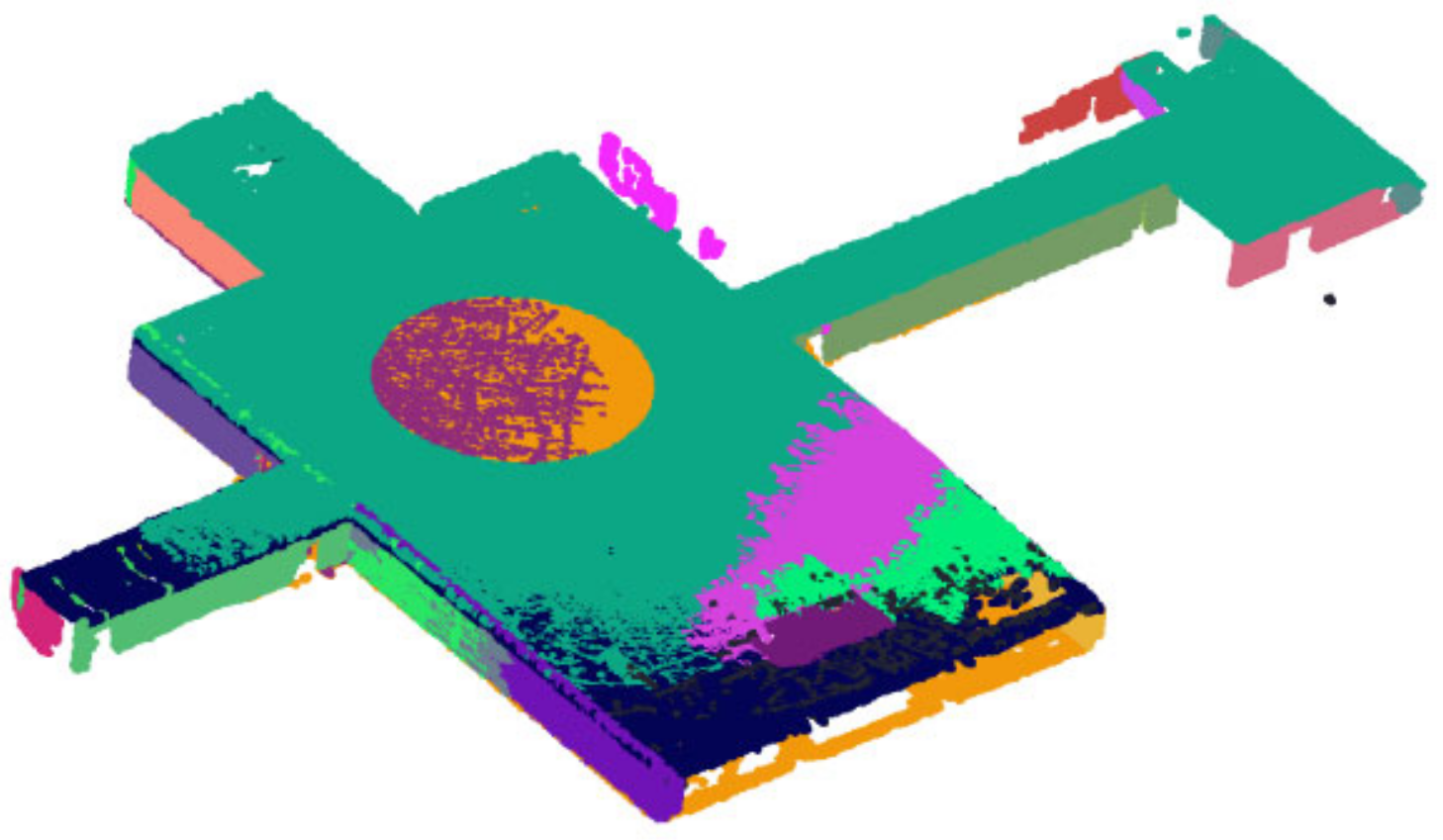
In Section 2.2, we segmented each plane accurately, but over-segmentation occurs at the same time during the experiment, as shown in Figure 9. As a result of equipment errors and algorithm errors, the plane made up of the point clouds is not a plane with only length and width, but also thickness; thus, a plane will be divided into multiple notional planes. Therefore, in the following section, the results of precise segmentation need to be optimized.

The exact plane obtained from Section 2.2 is:

$$\mathsf{{\rm P}}=\left\{{\mathrm{\Xi }}_1^{\prime },{\mathrm{\Xi }}_2^{\prime },\dots ,{\mathrm{\Xi }}_m^{\prime }\right\}$$

(18)

For each plane ${\mathrm{\Xi }}_i^{\prime }$, it is convenient to obtain the normal vector via PCA:

$${\nu }_i^{\prime }={\left(A_i^{\prime },B_i^{\prime },C_i^{\prime }\right)}^T$$

(19)

and the plane’s mathematical expression is:

$$A_i^{\prime }x+B_i^{\prime }y+C_i^{\prime }z+D_i^{\prime }=0,(i=1,2,\cdots ,m)$$

(20)

Then, the angle between ${\nu }_i^{\prime }$ and the normal vector of other planes is:

$${\theta }_{ij}=\arccos \left(\frac{|A_i{A}_j+B_i{B}_j+C_i{C}_j|}{\sqrt{A_i{}^2+B_i{}^2+C_i{}^2}\sqrt{A_j{}^2+B_j{}^2+C_j{}^2}}\right)$$

(21)

Setting a threshold $\vartheta$, when ${\theta }_{ij}<\vartheta$, we take the average to normalize the two normal vectors and calculate the distance between the two planes:

$$\left\{\begin{array}{l}{A}_i^{\prime }=A_j^{\prime }=\frac{A_i^{\prime }+A_j^{\prime }}{2}\\ B_i^{\prime }=B_j^{\prime }=\frac{B_i^{\prime }+B_j^{\prime }}{2}\\ C_i^{\prime }=C_j^{\prime }=\frac{C_i^{\prime }+C_j^{\prime }}{2}\end{array}\right.$$

(22)

$$d_{ij}=\frac{|D_i^{\prime }-D_j^{\prime }|}{\sqrt{{A_i^{\prime }}^2+{B_i^{\prime }}^2+{C_i^{\prime }}^2}}$$

(23)

Similarly, we take $d_0$ to be the distance threshold, and if $d_{ij}<d_0$, the two planes will be considered to belong to the same plane and normalized. The optimization cycle repeats until all planes are compared with other planes. Therefore, so far, the overall proposed algorithm stops.

3. Experimental Process and Results

In this section, we firstly introduce the acquisition equipment of the 3D LiDAR point cloud briefly. Next, we collect the point clouds of three indoor scenes from the real environment and obtain the raw data after filtering. To illustrate the feasibility and advantages of the method proposed in this paper, we selected several point cloud segmentation algorithms for comparison and displayed the results at the end.

3.1. 3D LiDAR Point Cloud Acquisition Equipment

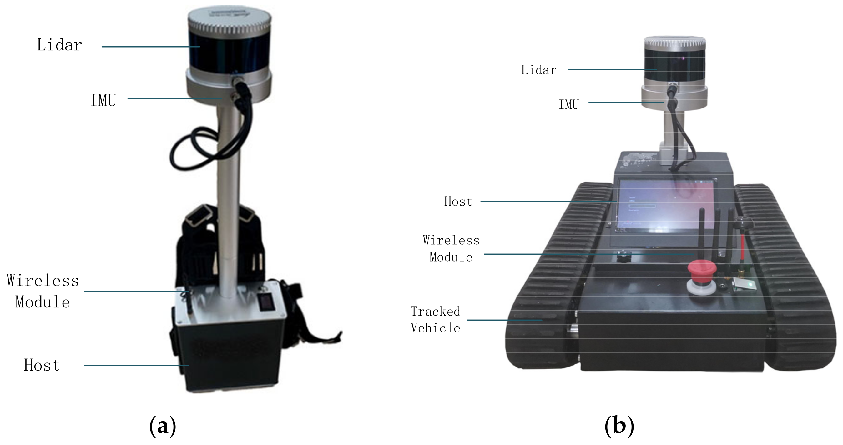
There are two kinds of hardware devices employed in our experiment, as shown in Figure 10. Figure 10a shows a three-dimensional point cloud reconstruction backpack, which is composed of a 16-line mechanical LiDAR, inertial measurement unit (IMU), wireless module and A lower computer. When collecting data, professional technicians are required to carry the equipment on and move slowly and at a constant speed within the measurement range in a stable attitude as much as possible. The other one is a 3D point cloud reconstruction trolley, shown in Figure 10b, which consists of a 16-line mechanical LiDAR, IMU, wireless module, lower computer and a crawler. When collecting data, the experimenter can control the movement of the car by operating the handle or planning the path so that the car can navigate autonomously and collect data.

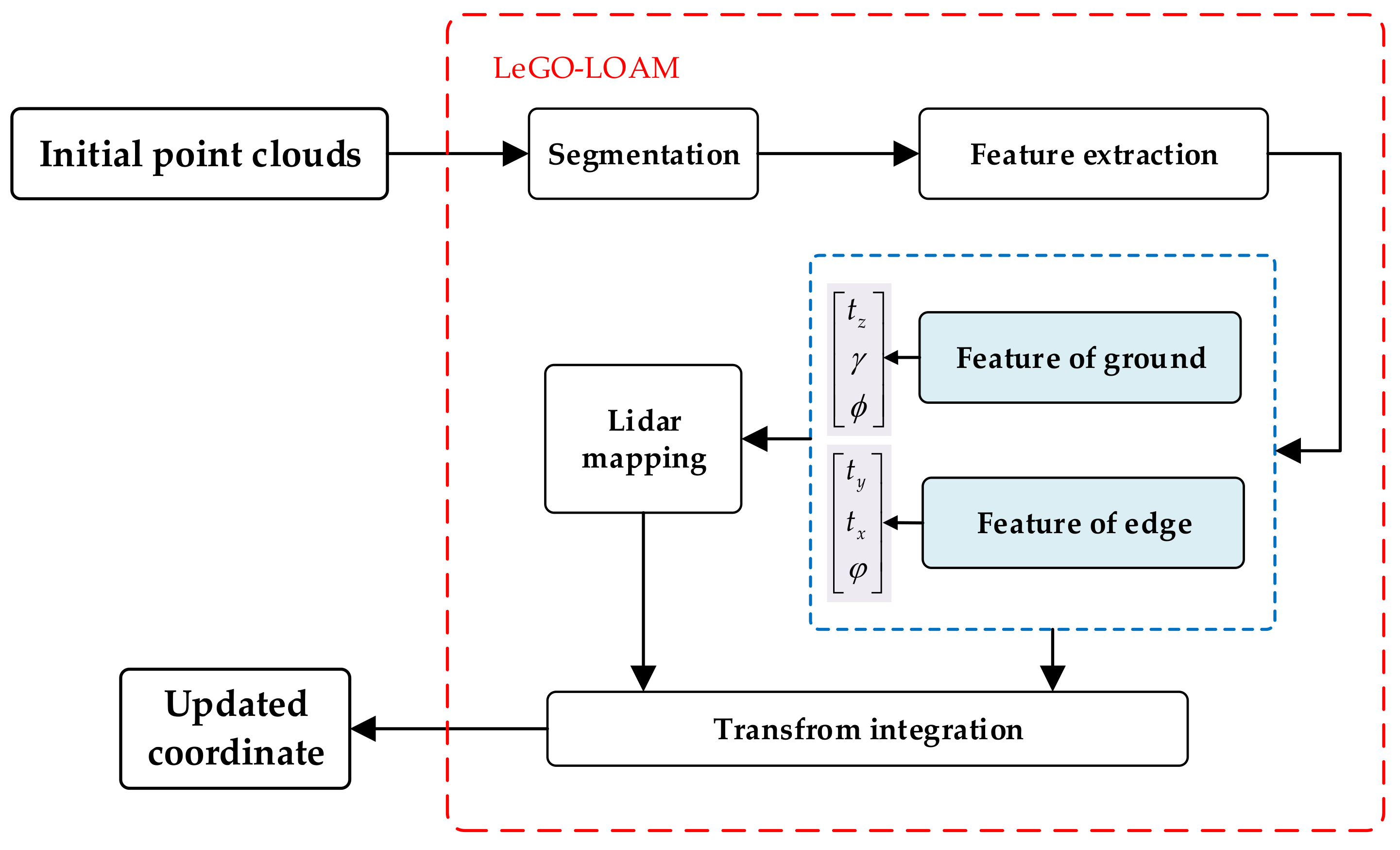
The principle of the equipment collecting data in the experiment is as follows: firstly, the experimenter starts the device, a wireless module connecting with a computer and scanning the surrounding environment at a speed of 0.5 s per frame. At the same time, the simultaneous localization and mapping (SLAM) program starts, and where the device started is the initial origin in the global coordinate system. Then, the point clouds scanned by LiDAR are transferred to the host for 3D reconstruction. In the 3D reconstruction, the coordinates are updated by matching the real-time IMU data with the point cloud of each frame via the LeGO-LOAM algorithm [42]. Finally, the updated coordinates are transmitted to the computer for real-time display through the wireless module.

The principle of the LeGO-LOAM algorithm is shown in Figure 11. The LeGO-LOAM algorithm first divides each frame of the initial point cloud into the ground point cloud and edge point cloud and extracts features from the two parts. Then, according to the ground features of the two frames before and after, the offset $t_z$, the roll angle $\gamma$ and the pitch angle $\varphi$ in the direction can be obtained, as well as the offset $t_y$, yaw angle $\phi$ in direction $y$ and offset $t_x$ in direction $x$. Therefore, the rotation and translation matrices of the two frames before and after can also be obtained, and the current global map can be updated.

3.2. Our Experiment Results in Three Scenes

To illustrate the applicability of our algorithm in various scenes, we collect the point clouds of the three scenes with different sizes and numbers of points with the equipment mentioned above. Due to the different scales of point clouds, the different distribution of the planes, the difference in the purpose of segmentation and the noise included, the relevant parameters in the experiment are different, as specifically shown in

Table 2. Parameter values of different parameters in three scenes in the algorithm.

Number of Scenes	${\mathit{\theta }}_0$	$\mathit{\lambda }$	$\mathit{r}$	${\mathit{N}}_{\mathit{x}}$	${\mathit{N}}_{\mathit{y}}$	$\mathit{R}$	$\mathit{N}$	$\mathit{\vartheta }$	${\mathit{d}}_0$
Scene 1	20	0.2	0.4	100	50	2	8	20	0.3
Scene 2	20	0.1	0.5	400	50	2	10	20	0.3
Scene 3	20	0.2	0.8	150	150	1.5	6	25	0.25

. The purpose of the proposed algorithm is to segment relatively larger planes in a scene, so we discard small planes such as tables, chairs, cabinets and computers (that is, considering the points of these planes as noise). The parameters in the table are:

${\theta }_0$ is the angle threshold of the normal vector between the seed voxel and the adjacent voxels in the rough segmentation; $\lambda$ is the distance threshold in rough segmentation to determine whether a point belongs to the extracted plane; $r$ represents the size of the voxels in Step.1; $N_x$ and $N_y$ are, respectively, the number of grids in $x$ and $y$ in precise segmentation; $R$ is the search radius of DBSCAN; $N$ is the minimum number of points contained within $R$; and $\vartheta$ $d_0$ are, respectively, the angle threshold and distance threshold in optimization.

• Scene 1

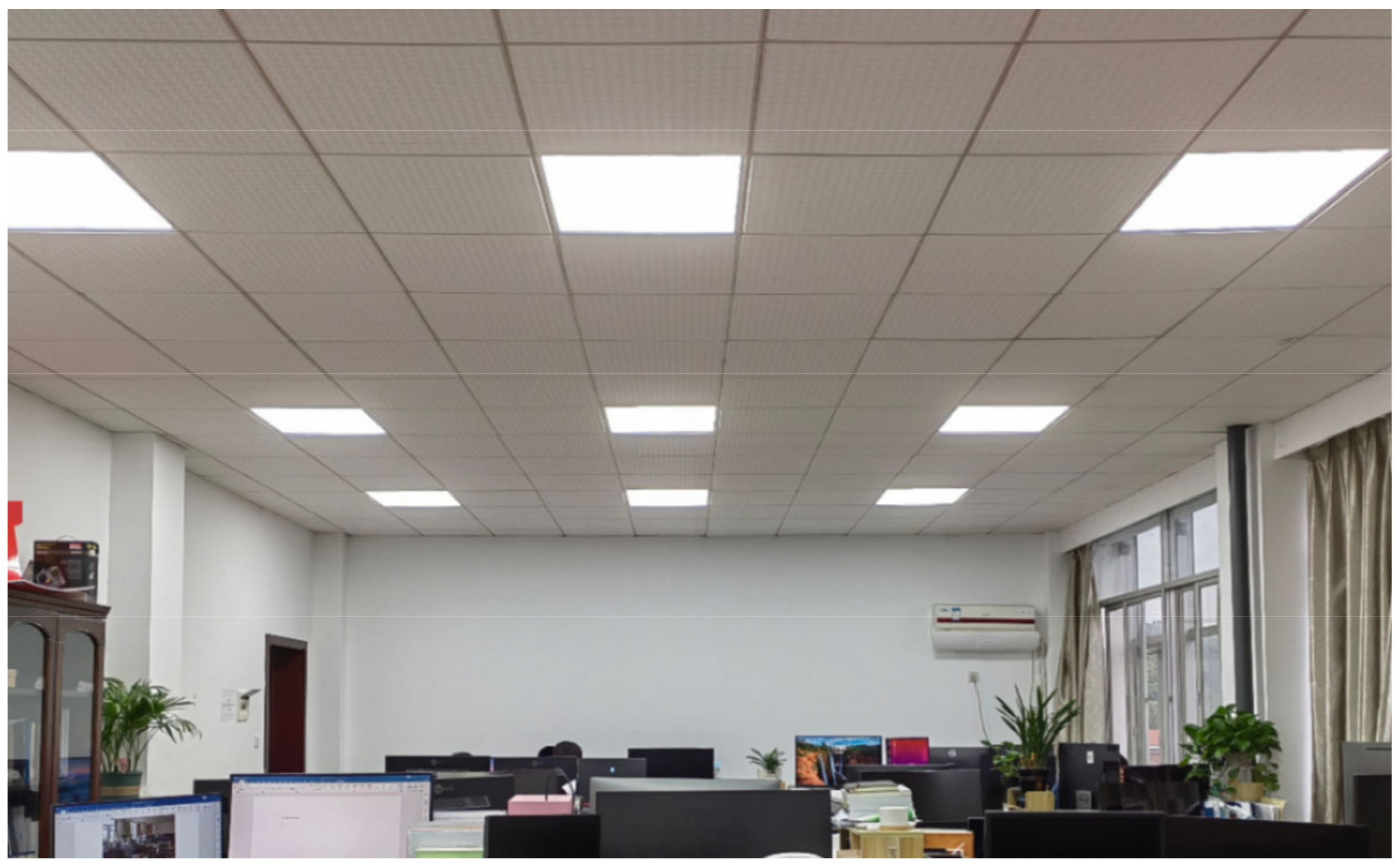
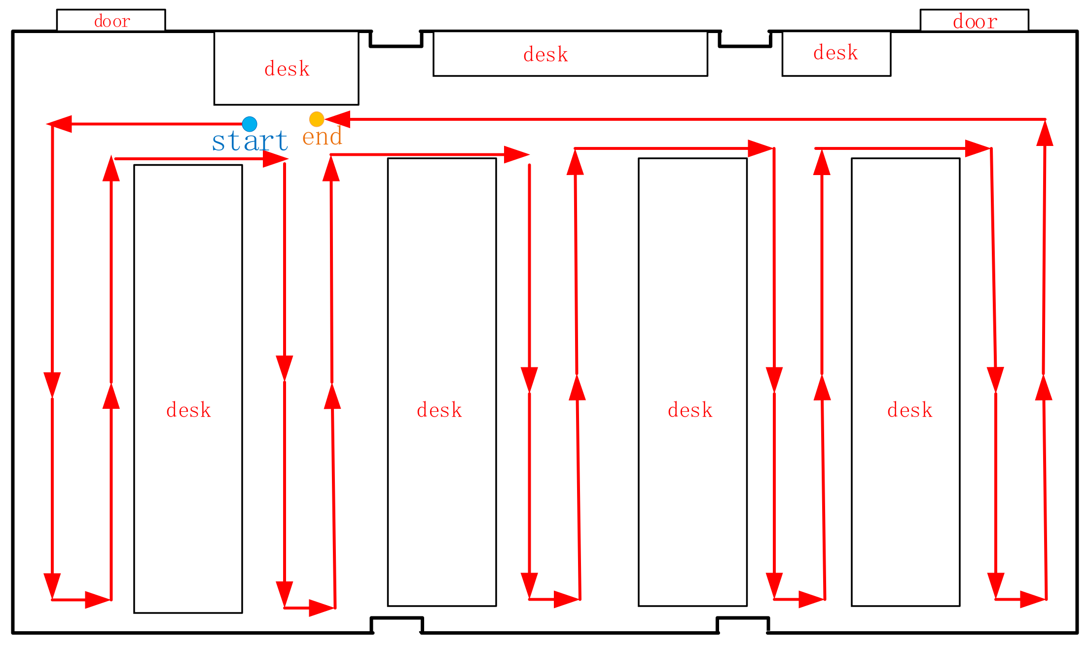
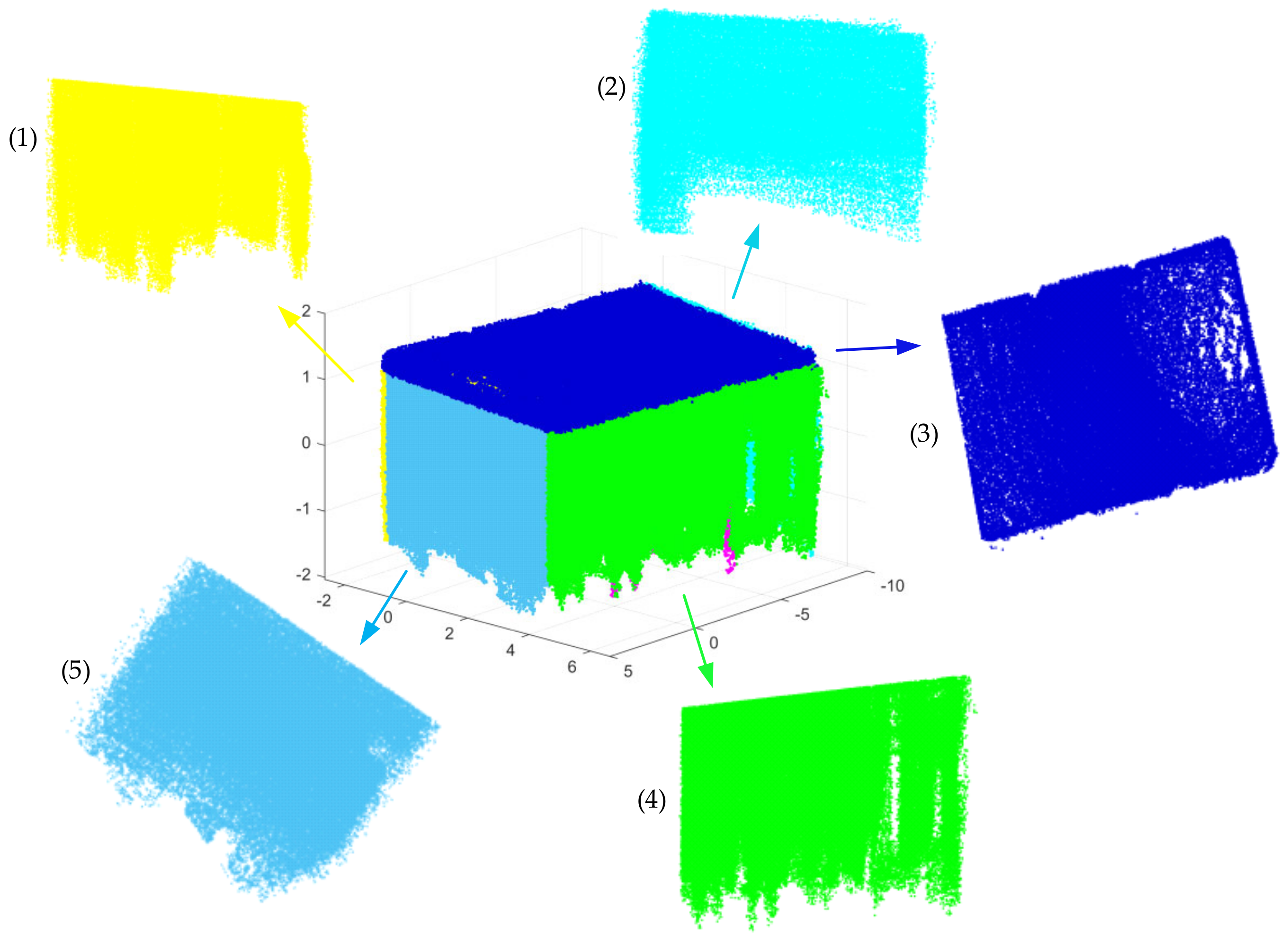
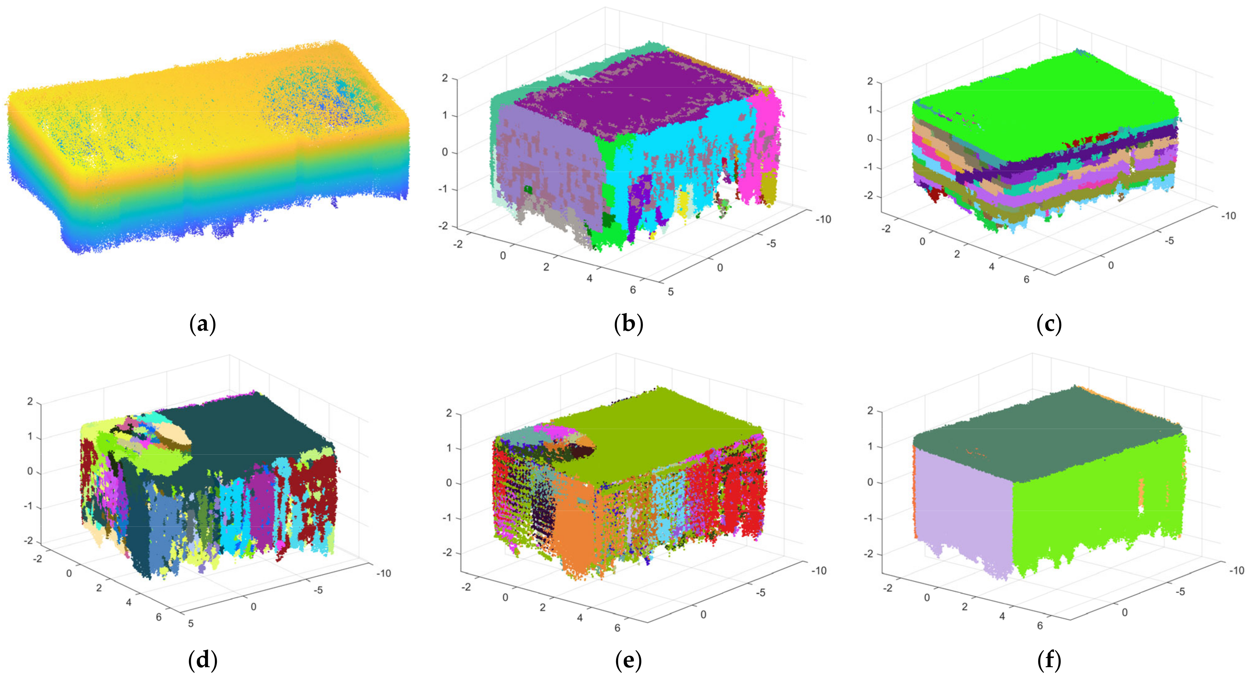
As shown in Figure 12, the point cloud of scene 1 comes from a single indoor room, and the data-collection path is shown in Figure 13. There are five planes with relatively uniform sizes that are perpendicular or parallel to each other, as distributed in scene 1. The first scene contains more than 820,369 points, as shown in Figure 14a. Figure 14b shows the precise segmentation result of scene 1, and it is obviously over-segmented. Figure 15 shows the final segmentation result after optimization.

• Scene 2

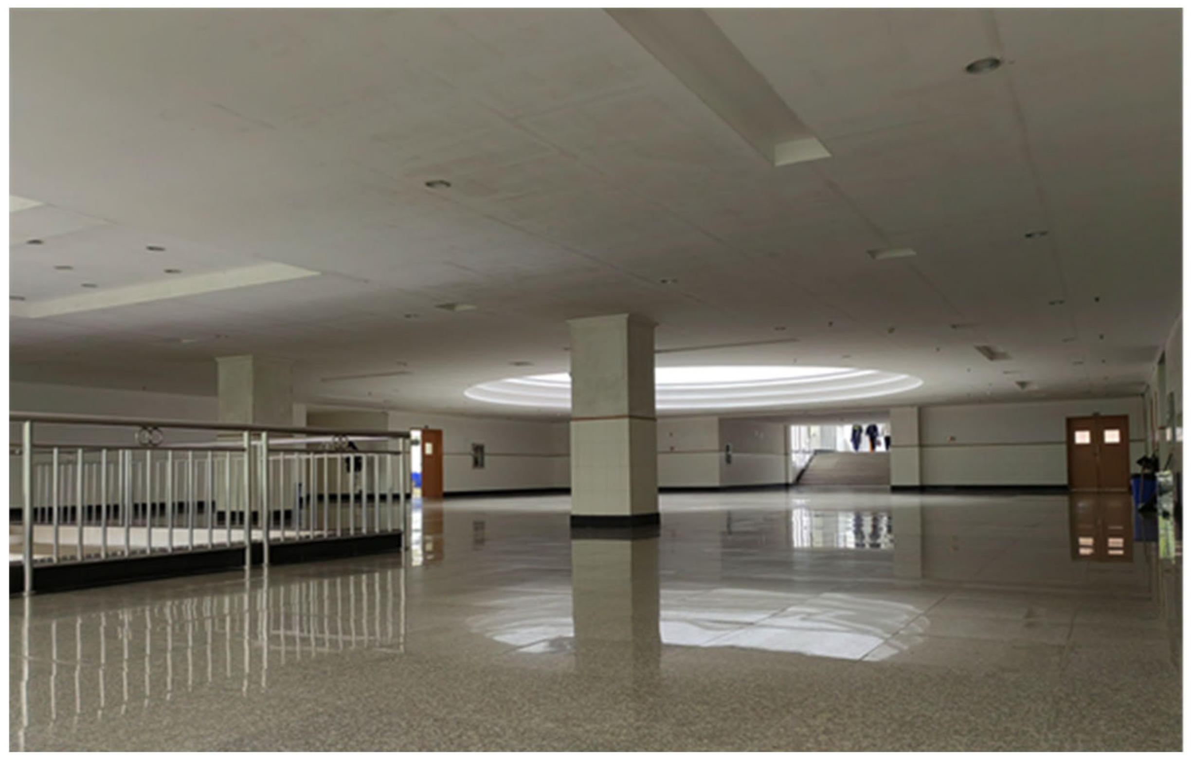
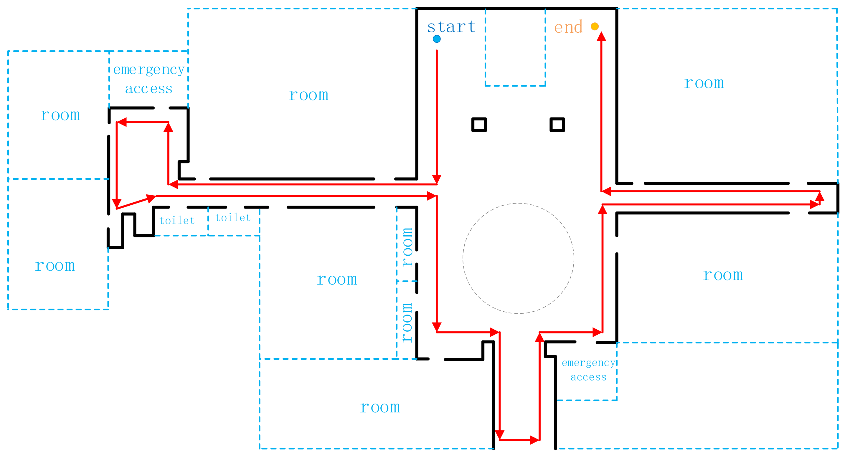
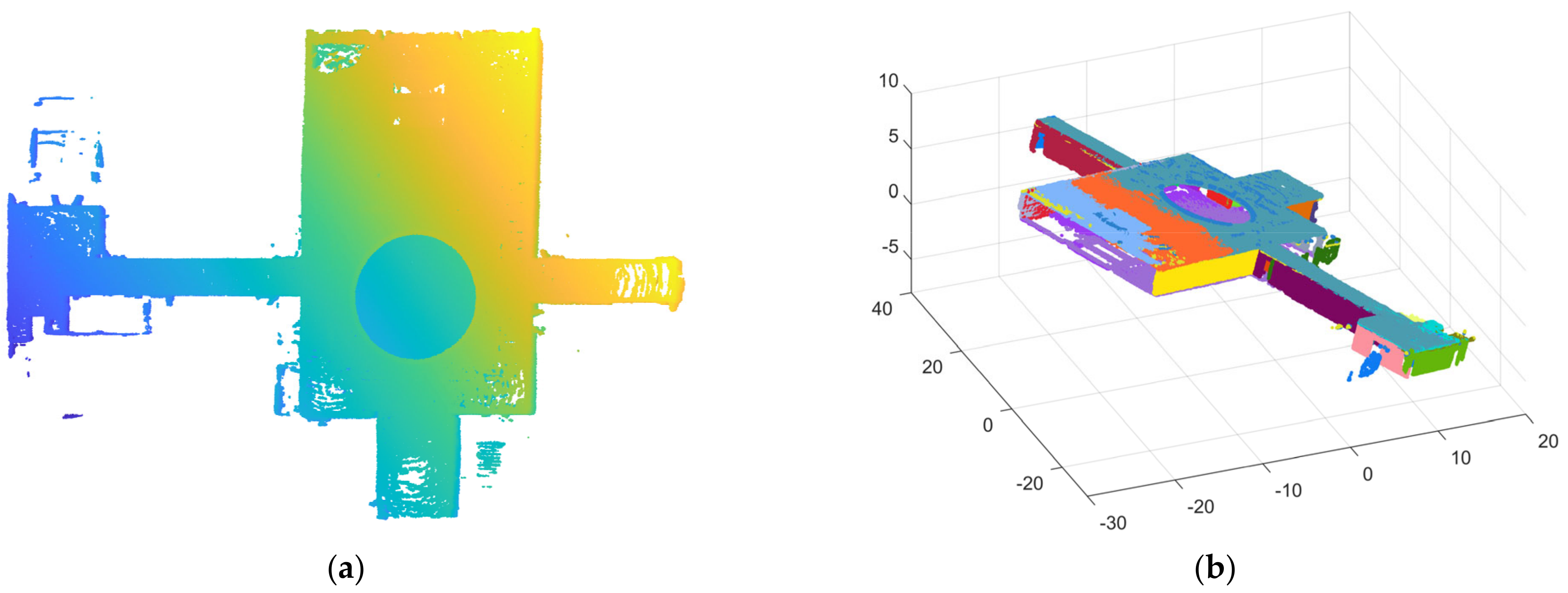
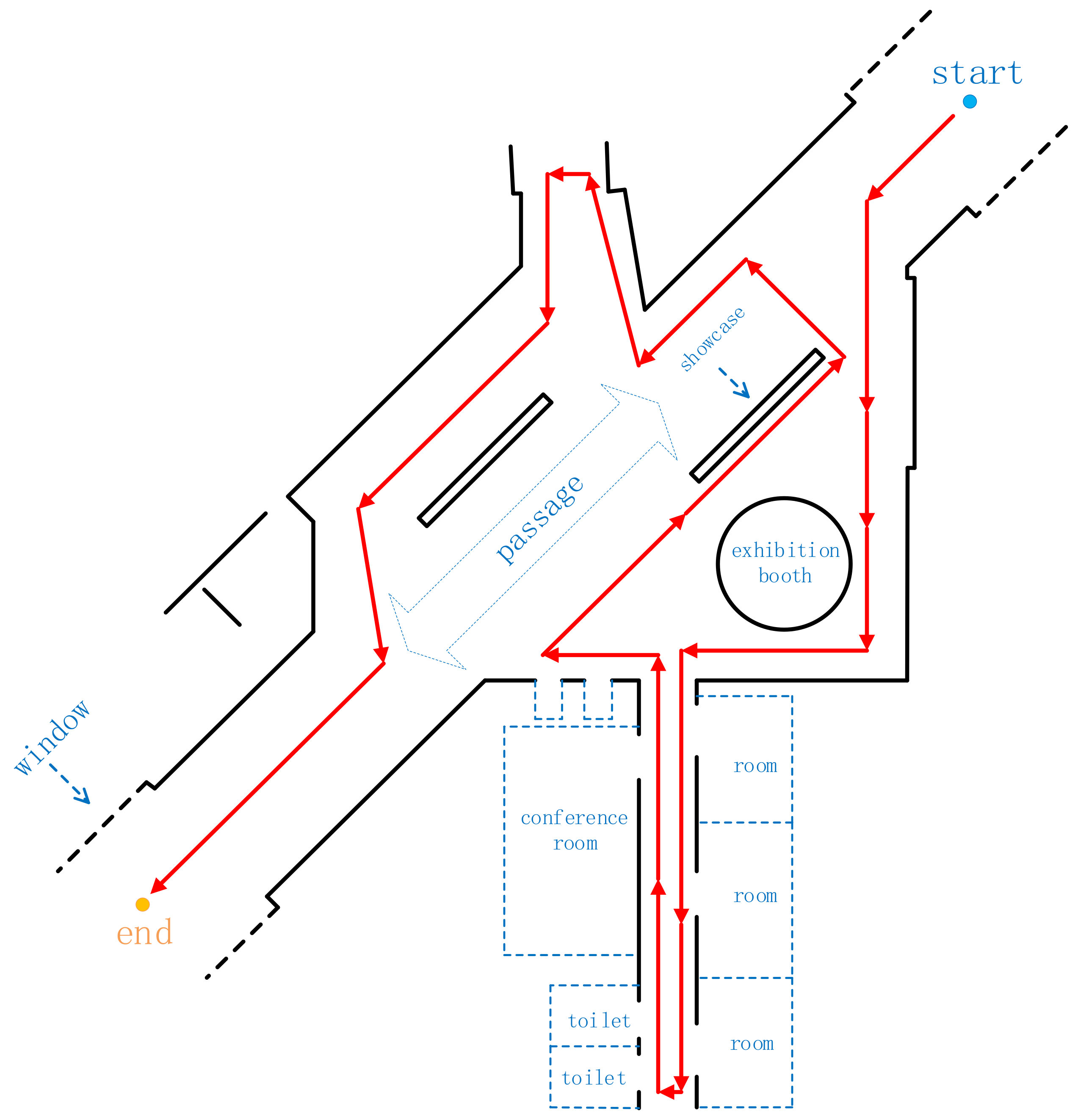
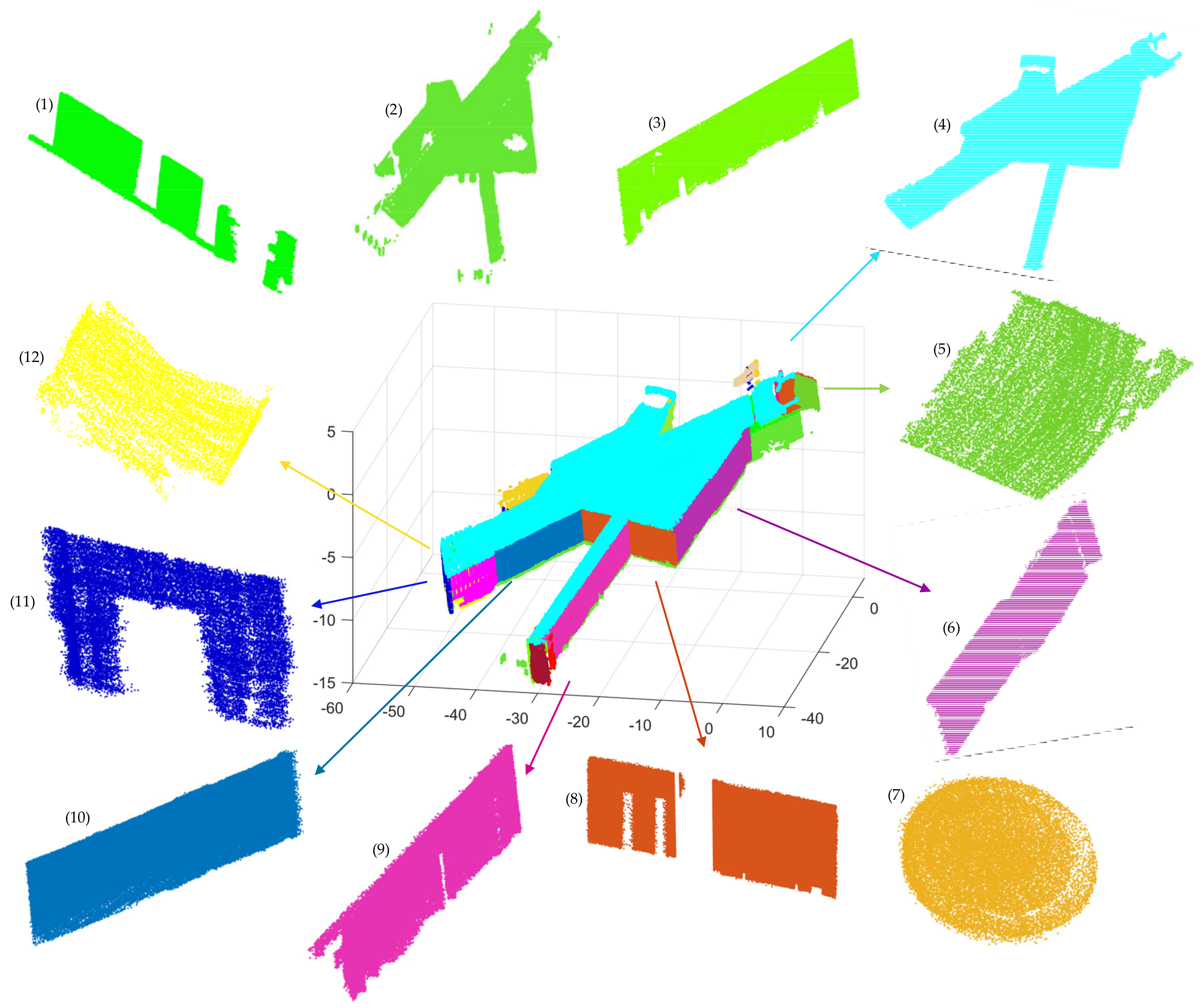
Scene 2 is a floor inside a building, as shown in Figure 16, and the data-collection path is shown in Figure 17. For some reason, the experimenters could not access the rooms along both sides of the corridors, but the effect of our algorithm in a single room is shown in scene 1. As shown in Figure 18a, the raw point cloud of scene 2 contains approximately 1.8 million points, including 22 visible planes. Here, we chose the large plane, which can be visually observed as the visual plane, to facilitate the subsequent parameter evaluation of our algorithm. Figure 18b shows the result of the algorithm precisely segmenting scene 2. The final segmentation result and part of the segmentation planes after optimization are shown in Figure 19.

• Scene 3

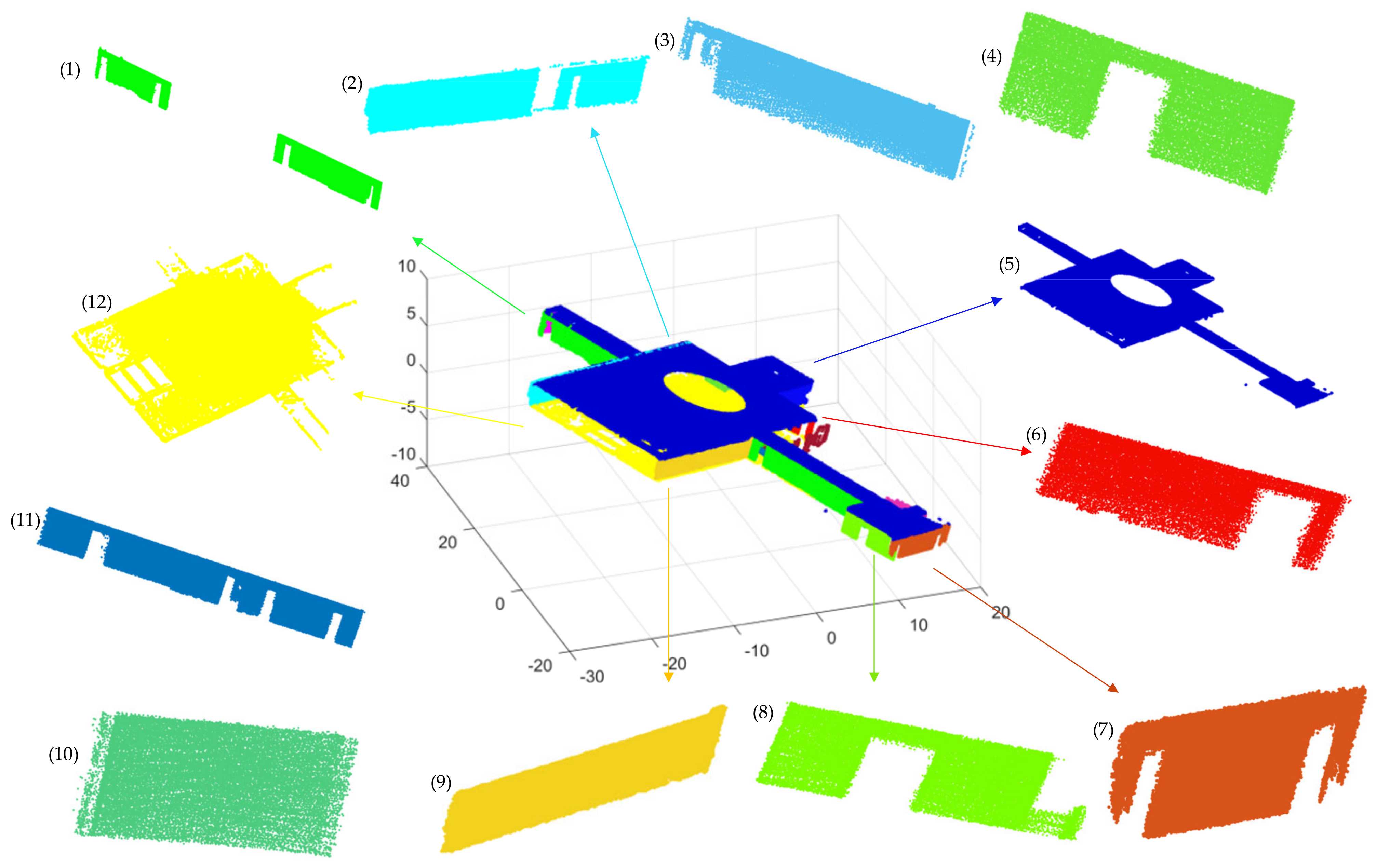
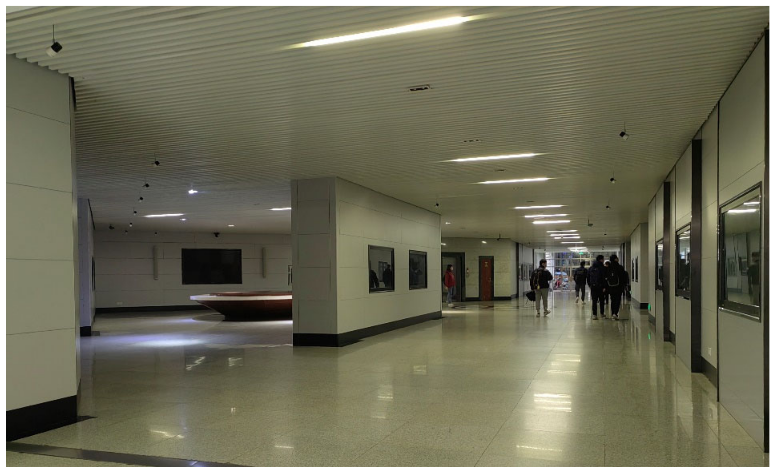
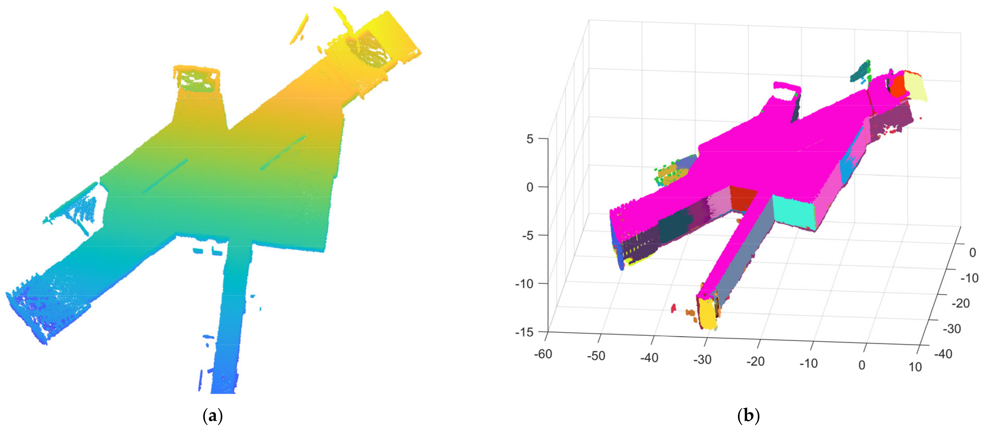
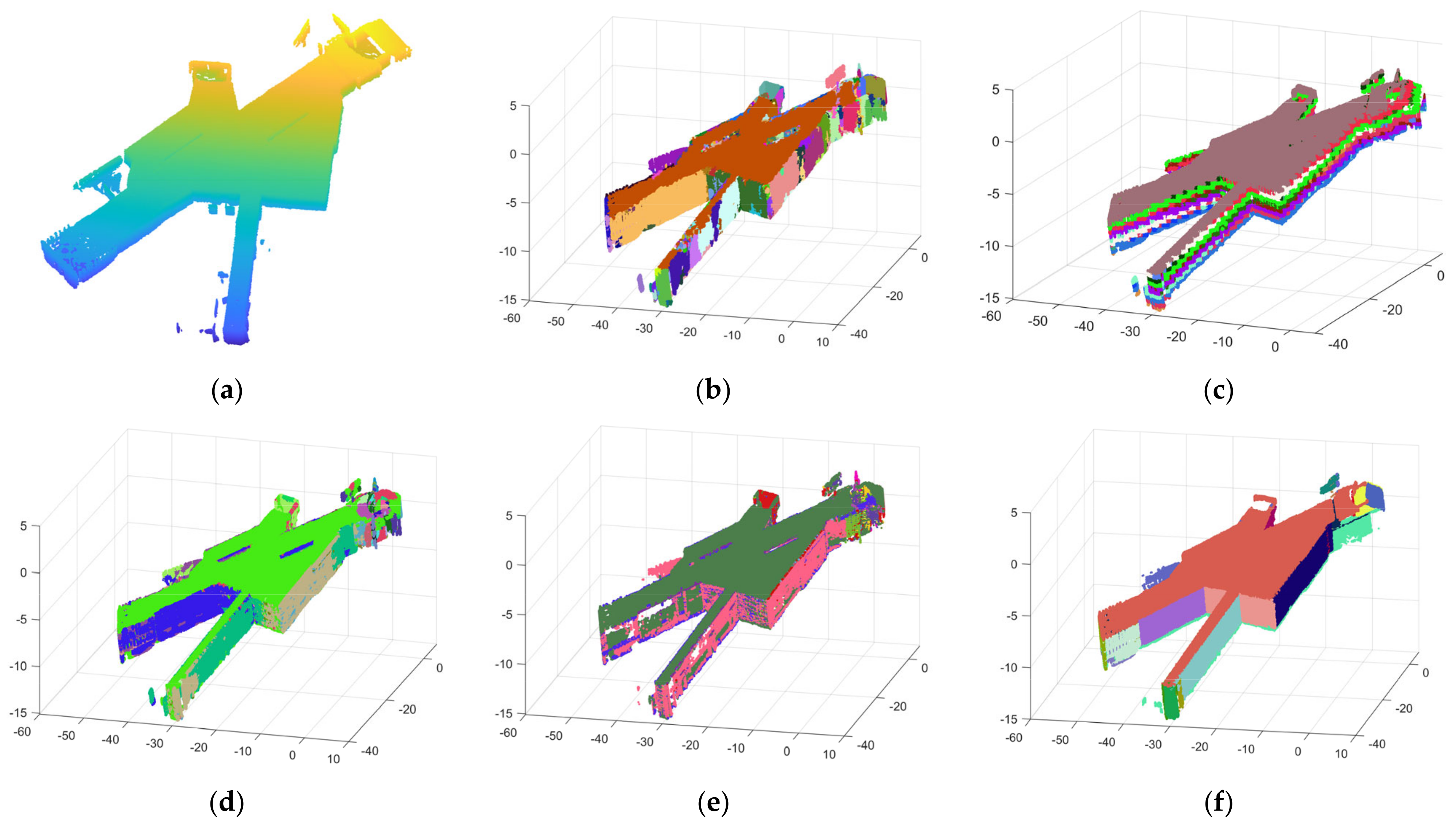
Scene 3 is a showroom with a long corridor, as shown in Figure 20. The data collected path of scene 3 are shown in Figure 21. As in scene 2, scene 3 does not contain single rooms, and mainly shows the plane segmentation effect of our algorithm in a larger indoor scene. Scene 3 contains approximately 2.8 million points, including 27 planes after filtering. Figure 22a shows the initial point cloud of scene 3, and (b) is the precise segmentation result of scene 3. Figure 23 shows the final segmentation result after optimization, as well as part of the segmented planes.

3.3. Comparison with Other Methods

Section 3.2 presents the segmentation effects of our method in three scenes. To quantitatively illustrate the efficiency and accuracy superiority of the proposed method, four segmentation algorithms were selected for comparison, which are the region growing (RG), random sample consensus (RANSAC), difference of normals (DoN) and normal $k$ nearest-neighbor (NKNN).

All the comparison algorithms run on the same device to minimize the impact of the processing device on the final segmentation result. At the same time, we also adjust the parameters in several contrasting methods to obtain relatively better segmentation results. After that, we obtained the segmentation results of four contrasting segmentation methods in three scenes. We introduce two parameters to evaluate the quality of the results namely time (T) and intersection-over-union (IoU), along with some intermediate parameters: true positive (TP), false positive (FP), false negative (FN) and error rate (ER). TP represents the correctly segmented planes, FP represents the samples that are non-planar but recognized as planes, and FN represents the samples that are planes but not recognized as planes. IoU is equal to the TP divided by the sum of TP, FP, and FN.

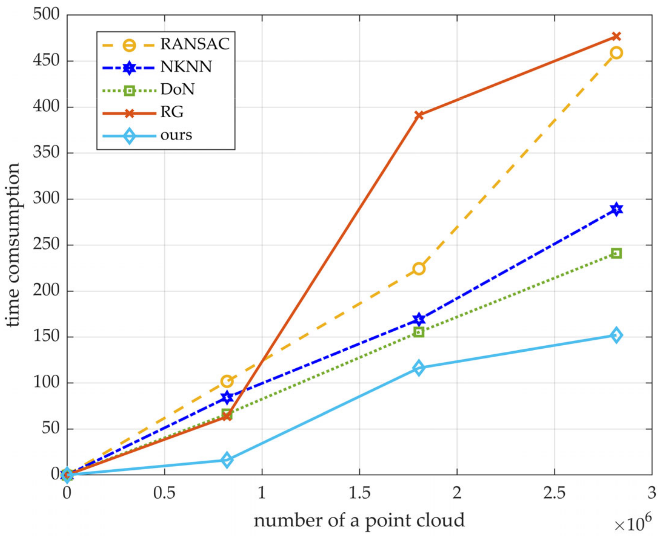
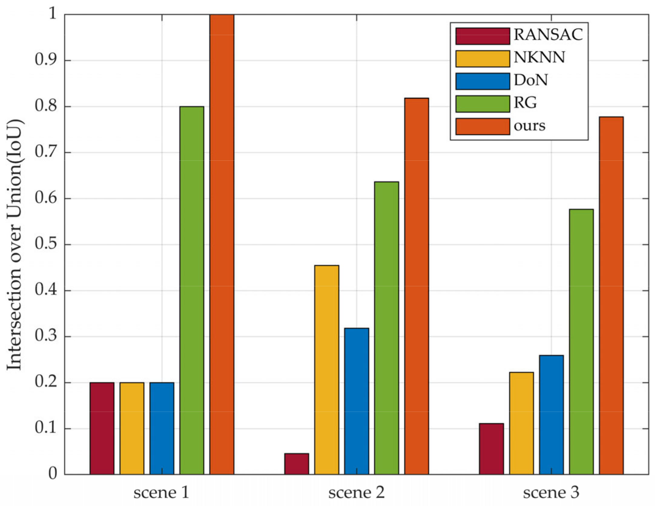
The results of the four methods for segmenting scene 1, scene 2, and scene 3 are shown in Figure 24, Figure 25 and Figure 26, respectively. The T, TP, FP, FN, IoU, and ER in the three scenarios are shown in

Table 3. T and IoU of five methods to segment Scene 1.

METHOD	T	TP	FP	FN	IoU	ER
RG	63.5465 s	4	0	1	0.8000	0.2000
RANSAC	101.8499 s	1	0	4	0.2000	0.8000
NKNN	84.2474 s	1	0	4	0.2000	0.8000
DoN	66.2764 s	1	0	4	0.2000	0.8000
Ours	16.2082 s	5	0	0	1.0000	0.0000

,

Table 4. T and IoU of five methods to segment Scene 2.

METHOD	T	TP	FP	FN	IoU	ER
RG	391.3039 s	14	0	8	0.6364	0.3636
RANSAC	224.3024 s	1	0	21	0.0455	0.9545
NKNN	169.0449 s	10	0	12	0.4545	0.5455
DoN	155.3330 s	7	0	15	0.3182	0.6818
Ours	116.4729 s	18	0	4	0.8182	0.1818

and

Table 5. T and IoU of five methods to segment Scene 3.

METHOD	T	TP	FP	FN	IoU	ER
RG	476.8546 s	15	0	11	0.5769	0.4231
RANSAC	459.1439 s	3	0	24	0.1111	0.8882
NKNN	288.8921 s	6	0	21	0.2222	0.7778
DoN	241.1156 s	7	0	20	0.2593	0.7407
Ours	152.0937 s	21	1	5	0.7778	0.2222

, respectively. Figure 27 shows the variety of the processing time of the four segmentation methods along with a variety of the number of points in the scenes. Figure 28 shows the IoU of the segmentation results more intuitively by exchanging tables into a bar chart.

4. Discussion

To more scientifically evaluate the advantages and disadvantages of our algorithm, in this section, we will focus on the following two aspects: the experimental results of plane segmentation and the quantitative analysis of parameters.

As for the experimental results, first of all, the precise segmentation results of our algorithm are shown in Figure 14b, Figure 18b and Figure 22b. It is obvious that planes are almost completely segmented. However, due to the thickness of the point clouds, there is over-segmentation in precise segmentation. The results after optimization are shown in Figure 15, Figure 19 and Figure 23. A single plane in the scenes can be completely extracted, and we can easily distinguish each plane in the final segmentation result, which illustrates that our algorithm performs well in segmenting indoor point cloud planes. In addition, it can be seen in Figure 24, Figure 25 and Figure 26 that although the comparison algorithms can also extract partial planes, they are often not complete or accurate. Undersegmentation (RG), unidirectional segmentation plane (RANSAC), dividing a plane into multiple planes (NKNN), plane loss (DoN) and containing more noise points are obvious. In contrast, Figure 24f, Figure 25f and Figure 26f intuitively illustrate that our algorithm outperforms the four comparison algorithms in both the completeness and quantity of the extracted planes.

As for the experimental parameters, the efficiency and accuracy of our algorithm are both better than the comparison algorithms. In Table 3, the processing time to segment scene 1 is 63.5465s (RG), 101.8499s (RANSAC), 84.2474s (NKNN), 66.2764s (DoN), and 16.2082s (ours). Obviously, it is quicker to segment scene 1 for our method than the other four algorithms, and the same conclusion can be drawn from the results in scene 2 and scene 3 (Table 4 and Table 5). We take T as a function of the number of point clouds in scenes, as shown in Figure 27. As the number of points increases, the processing time increases to varying degrees as well, and RG increases the most, while our algorithm increases the most gently. Furthermore, the plane segmentation accuracy of our algorithm is higher than the other four methods. By observing Figure 28, visualized by the relevant parameters in Table 3, Table 4 and Table 5, it is apparent that the IoU of four comparison algorithms varies greatly with the environment, while our algorithm can reach 0.8182 and 0.7778, respectively, in scene 2 (with 22 planes) and scene 3 (with 27 planes) where the environment is complex. Even if the IoU decreases slightly as scenes become more complex, it is still much higher than the other three methods in general.

In addition, our algorithm has some shortcomings: it is difficult to formulate parameters that satisfy both large and small plane segmentation. When scenes are extremely complex, or the size of the planes that need to be extracted varies too much, our algorithm may not achieve the results we expect.

5. Conclusions

This paper proposed a fast and precise plane segmentation framework for indoor point clouds. The core steps of the algorithm are divided into two steps: plane rough segmentation and precise segmentation. Firstly, the raw data are voxelized; then, the rough segmentation is realized according to the angle of the local normal vector between the seed voxel and the nearest-neighbor voxels. Secondly, the precise segmentation algorithm based on DBSCAN is adopted to achieve the precise extraction of the plane. Finally, the final extraction planes are obtained by optimizing the results to overcome over-segmentation. By analyzing the experimental results and relevant parameters, our algorithm signDificantly outperforms the compared algorithms in terms of both efficiency and accuracy. However, our algorithm cannot extract planes in extremely different sizes at the same time, and the algorithm needs to be further optimized in follow-up work.

References

1. Zong, W.P.; Li, G.Y.; Li, M.L.; Wang, L.; Li, S.X. A survey of laser scan matching methods. Chin. Opt. 2018, 11, 914–930. [Google Scholar] [CrossRef]
2. Zhong, H.; Wang, H.; Wu, Z.; Zhang, C.; Zheng, Y.; Tang, T. A survey of LiDAR and camera fusion enhancement. Procedia Comput. Sci. 2021, 183, 579–588. [Google Scholar] [CrossRef]
3. Fernandes, D.; Silva, A.; Névoa, R.; Simões, C.; Gonzalez, D.; Guevara, M.; Novais, P.; Monteiro, J.; Melo-Pinto, P. Point-cloud based 3D object detection and classification methods for self-driving applications: A survey and taxonomy. Inf. Fusion 2021, 68, 161–191. [Google Scholar] [CrossRef]
4. Benedek, C.; Majdik, A.; Nagy, B.; Rozsa, Z.; Sziranyi, T. Positioning and perception in LIDAR point clouds. Digit. Signal Process. 2021, 119, 103193. [Google Scholar] [CrossRef]
5. Zamanakos, G.; Tsochatzidis, L.; Amanatiadis, A.; Pratikakis, I. A comprehensive survey of LIDAR-based 3D object detection methods with deep learning for autonomous driving. Comput. Graph. 2021, 99, 153–181. [Google Scholar] [CrossRef]
6. Lin, Y.F.; Yang, L.J.; Yu, C.Y.; Peng, C.C.; Huang, D.C. Object Recognition and Classification of 2D-SLAM Using Machine Learning and Deep Learning Techniques. In Proceedings of the 2020 International Symposium on Computer, Consumer and Control (IS3C), Taichung City, Taiwan, 13–16 November 2020; pp. 473–476. [Google Scholar] [CrossRef]
7. Lee, S.W.; Hsu, C.M.; Lee, M.C.; Fu, Y.T.; Atas, F.; Tsai, A. Fast Point Cloud Feature Extraction for Real-time SLAM. In Proceedings of the 2019 International Automatic Control Conference (CACS), Keelung, Taiwan, 13–16 November 2019; pp. 1–6. [Google Scholar]
8. Fan, Y.; Zhang, Q.; Liu, S.; Tang, Y.; Jing, X.; Yao, J.; Han, H. Semantic SLAM with More Accurate Point Cloud Map in Dynamic Environments. IEEE Access 2020, 8, 112237–112252. [Google Scholar] [CrossRef]
9. Isa, S.N.M.; Shukor, S.A.A.; Rahim, N.A.; Maarof, I.; Yahya, Z.R.; Zakaria, A.; Abdullah, A.H.; Wong, R. A Review of Data Structure and Filtering in Handling 3D Big Point Cloud Data for Building Preservation. In Proceedings of the 2018 IEEE Conference on Systems, Process and Control (ICSPC), Melaka, Malaysia, 14–15 December 2018. [Google Scholar]
10. Kurup, S.; Bhise, A. A Systematic Review of Automated Reconstruction of Indoor Scenes using Point Clouds. In Proceedings of the 2021 International Conference on Image, Video Processing, and Artificial Intelligence, Shanghai, China, 23–24 October 2021. [Google Scholar] [CrossRef]
11. Xu, Y.S.; Stilla, U. Toward Building and Civil Infrastructure Reconstruction from Point Clouds: A Review on Data and Key Techniques. IEEE J. Sel. Top. Appl. Earth Obs. Remote Sens. 2021, 14, 2857–2885. [Google Scholar] [CrossRef]
12. Wang, R.S.; Peethambaran, J.; Chen, D. LiDAR Point Clouds to 3-D Urban Models: A Review. IEEE J. Sel. Top. Appl. Earth Obs. Remote Sens. 2018, 11, 606–627. [Google Scholar] [CrossRef]
13. Cheng, D.Y.; Zhang, J.C.; Zhao, D.J.; Chen, J.L.; Tian, D. Automatic Extraction of Indoor Structural Information from Point Clouds. Remote Sens. 2021, 13, 4930. [Google Scholar] [CrossRef]
14. Wang, X.Y.; Xiao, J.; Wang, Y. Research of Plane Extraction Methods based on Region Growing. In Proceedings of the 2016 International Conference on Virtual Reality and Visualization, Hangzhou, China, 24–26 September 2016; pp. 298–303. [Google Scholar] [CrossRef]
15. Leng, X.X.; Xiao, J.; Wang, Y. A multi-scale plane-detection method based on the Hough transform and region growing. Photogramm. Rec. 2016, 31, 166–192. [Google Scholar] [CrossRef]
16. Xiao, J.; Zhang, J.; Adler, B.; Zhang, H.; Zhang, J. Three-dimensional point cloud plane segmentation in both structured and unstructured environments. Robot. Auton. Syst. 2013, 61, 1641–1652. [Google Scholar] [CrossRef]
17. Fischler, M.A.; Bolles, R.C. Random Sample Consensus: A Paradigm for Model Fitting with Applications to Image Analysis and Automated Cartography. In Readings in Computer Vision; Fischler, M.A., Firschein, O., Eds.; Morgan Kaufmann: San Francisco, CA, USA, 1987; pp. 726–740. [Google Scholar]
18. Schnabel, R.; Wahl, R.; Klein, R. Efficient RANSAC for Point-Cloud Shape Detection. Comput. Gr. Forum 2007, 26, 214–226. [Google Scholar] [CrossRef]
19. Ioannou, Y.; Taati, B.; Harrap, R.; Greenspan, M. Difference of Normals as a Multi-scale Operator in Unorganized Point Clouds. In Proceedings of the 2012 Second International Conference on 3D Imaging, Modeling, Processing, Visualization & Transmission, Zurich, Switzerland, 13–15 October 2012; pp. 501–508. [Google Scholar]
20. Xu, S.; Wang, R.; Wang, H.; Yang, R. Plane Segmentation Based on the Optimal-Vector-Field in LiDAR Point Clouds. IEEE Trans. Pattern Anal. Mach. Intell. 2021, 43, 3991–4007. [Google Scholar] [CrossRef] [PubMed]
21. Lunkai, Z.; Junguo, L.; Yubin, M. A New Effective Parallel Plane Segmentation Method for Point Cloud Based on Dimension Reduction Correction. In Proceedings of the 2020 Chinese Control and Decision Conference (CCDC), Piscataway, NJ, USA, 22–24 August 2020; pp. 1877–1882. [Google Scholar]
22. Cheng, D.Y.; Zhao, D.J.; Zhang, J.C.; Wei, C.S.; Tian, D. PCA-Based Denoising Algorithm for Outdoor Lidar Point Cloud Data. Sensors 2021, 21, 3703. [Google Scholar] [CrossRef]
23. Ester, M.; Kriegel, H.P.; Sander, J.; Xu, X. A Density-Based Algorithm for Discovering Clusters in Large Spatial Databases with Noise. Kdd 1996, 96, 226–231. [Google Scholar]
24. Ram, A.; Sunita, J.; Jalal, A.; Manoj, K. A Density Based Algorithm for Discovering Density Varied Clusters in Large Spatial Databases. Int. J. Comput. Appl. 2010, 3, 1–4. [Google Scholar] [CrossRef]
25. Li, P.; Wang, R.S.; Wang, Y.X.; Gao, G. Automated Method of Extracting Urban Roads Based on Region Growing from Mobile Laser Scanning Data. Sensors 2019, 19, 5262. [Google Scholar] [CrossRef] [Green Version]
26. Su, Z.; Gao, Z.; Zhou, G.; Li, S.; Song, L.; Lu, X.; Kang, N. Building Plane Segmentation Based on Point Clouds. Remote Sens. 2021, 14, 95. [Google Scholar] [CrossRef]
27. Dong, Z.; Yang, B.; Hu, P.; Scherer, S. An efficient global energy optimization approach for robust 3D plane segmentation of point clouds. ISPRS J. Photogramm. Remote Sens. 2018, 137, 112–133. [Google Scholar] [CrossRef]
28. Zhang, X.M.; Wan, W.G.; Xiao, L.; Ma, J.X. Mean Shift Clustering Segmentation and RANSAC Simplification of Color Point Cloud. In Proceedings of the 2014 International Conference on Audio, Language and Image Processing (Icalip), Shanghai, China, 7–9 July 2014; Volume 1–2, pp. 837–841. [Google Scholar]
29. Xu, B.; Jiang, W.S.; Shan, J.; Zhang, J.; Li, L.L. Investigation on the Weighted RANSAC Approaches for Building Roof Plane Segmentation from LiDAR Point Clouds. Remote Sens. 2016, 8, 5. [Google Scholar] [CrossRef] [Green Version]
30. Yuan, H.N.; Sun, W.; Xiang, T.Y. Line laser point cloud segmentation based on the combination of RANSAC and region growing. In Proceedings of the 2020 39th Chinese Control Conference (CCC), Shenyang, China, 27–30 July 2020; pp. 6324–6328. [Google Scholar]
31. Xu, D.; Li, F.H.; Wei, H.X. 3D Point Cloud Plane Segmentation Method Based on RANSAC and Support Vector Machine. In Proceedings of the 2019 14th IEEE Conference on Industrial Electronics and Applications (ICIEA), Xi’an, China, 19–21 June 2019; pp. 943–948. [Google Scholar]
32. Yang, L.N.; Li, Y.C.; Li, X.C.; Meng, Z.Q.; Luo, H.W. Efficient plane extraction using normal estimation and RANSAC from 3D point cloud. Comput. Stand. Interfaces 2022, 82, 103608. [Google Scholar] [CrossRef]
33. Xu, Y.; Tong, X.; Stilla, U. Voxel-based representation of 3D point clouds: Methods, applications, and its potential use in the construction industry. Autom. Constr. 2021, 126, 103675. [Google Scholar] [CrossRef]
34. Wei, P.C.; Yan, L.; Xie, H.; Huang, M. Automatic coarse registration of point clouds using plane contour shape descriptor and topological graph voting. Autom. Constr. 2022, 134, 104055. [Google Scholar] [CrossRef]
35. Huang, M.; Wei, P.C.; Liu, X.L. An Efficient Encoding Voxel-Based Segmentation (EVBS) Algorithm Based on Fast Adjacent Voxel Search for Point Cloud Plane Segmentation. Remote Sens. 2019, 11, 2727. [Google Scholar] [CrossRef] [Green Version]
36. Xu, Y.; Ye, Z.; Huang, R.; Hoegner, L.; Stilla, U. Robust segmentation and localization of structural planes from photogrammetric point clouds in construction sites. Autom. Constr. 2020, 117, 103206. [Google Scholar] [CrossRef]
37. Lee, H.; Jung, J. Clustering-Based Plane Segmentation Neural Network for Urban Scene Modeling. Sensors 2021, 21, 8382. [Google Scholar] [CrossRef]
38. Saglam, A.; Makineci, H.B.; Baykan, N.A.; Baykan, O.K. Boundary constrained voxel segmentation for 3D point clouds using local geometric differences. Expert Syst. Appl. 2020, 157, 113439. [Google Scholar] [CrossRef]
39. Vo, A.V.; Linh, T.H.; Laefer, D.F.; Bertolotto, M. Octree-based region growing for point cloud segmentation. Isprs J. Photogramm. Remote Sens. 2015, 104, 88–100. [Google Scholar] [CrossRef]
40. Czerniawski, T.; Sankaran, B.; Nahangi, M.; Haas, C.; Leite, F. 6D DBSCAN-based segmentation of building point clouds for planar object classification. Autom. Constr. 2018, 88, 44–58. [Google Scholar] [CrossRef]
41. Chen, H.; Liang, M.; Liu, W.; Wang, W.; Liu, P.X. An approach to boundary detection for 3D point clouds based on DBSCAN clustering. Pattern Recognit. 2022, 124, 108431. [Google Scholar] [CrossRef]
42. Shan, T.; Englot, B. LeGO-LOAM: Lightweight and Ground-Optimized Lidar Odometry and Mapping on Variable Terrain. In Proceedings of the 2018 IEEE/RSJ International Conference on Intelligent Robots and Systems (IROS), Madrid, Spain, 1–5 October 2018; pp. 4758–4765. [Google Scholar]
Figure 1. The overall flow chart of the proposed algorithm.
Remotesensing 14 03519 g001
Figure 2. The flow chart of the rough segmentation of the initial point cloud.
Remotesensing 14 03519 g002
Figure 3. Point cloud voxelization: (a) raw data; (b) voxelization with r = 4 ; (c) voxelization with r = 2 ; (d) voxelization with r = 1 . The parameter r is the size of voxels.
Remotesensing 14 03519 g003
Figure 4. Two distributions of adjacent voxels of seed voxels. Each small square represents a voxel.
Remotesensing 14 03519 g004
Figure 5. Single-pass plane determination process for normal vectors. When all voxels meet the conditions, the plane will be determined depending on the points in all the current voxels via the least-squares method, and the normal vector is obtained via PCA. Finally, the points in the final plane are determined according to the distance from the points to the plane.
Remotesensing 14 03519 g005
Figure 6. Algorithmic process of DBSCAN. Here N = 5. In the left, A , is the initial core density point and B , C , D , E , contained in the radius of A are the points meeting the density condition, the other colored points are contained in B , C , D , E but don’t meet the condition. Therefore in the right, A , B , C , D , E and the points they contained are classified as one category colored red, while the outliers are colored black.
Remotesensing 14 03519 g006
Figure 7. Algorithm process of precise segmentation based on DBSCAN.
Remotesensing 14 03519 g007
Figure 8. Process of the grid being marked.
Remotesensing 14 03519 g008
Figure 9. Over-segmentation in plane segmentation.
Remotesensing 14 03519 g009
Figure 10. (a) Three-dimensional reconstruction backpack. (b) Three-dimensional reconstruction trolley.
Remotesensing 14 03519 g010
Figure 11. The principle of the LeGO-LOAM algorithm.
Remotesensing 14 03519 g011
Figure 12. The real scene of scene 1.
Remotesensing 14 03519 g012
Figure 13. The data-collection path of scene 1 (with arrows).
Remotesensing 14 03519 g013
Figure 14. (a) The raw point cloud of scene 1; and (b) the result of precise segmentation.
Remotesensing 14 03519 g014
Figure 15. The final segmentation result after the optimization and several planes of scene 1. The separate planes labeled (15), respectively, correspond to the plane with the same color in scene 1; (3), (4) and (5) are visible, while (1) and (2) are invisible here.
Remotesensing 14 03519 g015
Figure 16. The real scene of scene 2.
Remotesensing 14 03519 g016
Figure 17. The data collected path of scene 2 (along with the arrow). The blue dashed boxes represent inaccessible rooms and areas, which are not included in the raw point cloud. The grey dotted line represents a circular cutout in the ceiling, visible in Figure 16.
Remotesensing 14 03519 g017
Figure 18. (a) The raw point cloud of scene 2; and (b) the result of precise segmentation.
Remotesensing 14 03519 g018
Figure 19. The final segmentation result after optimization and several segmentation planes of scene 2. The separate planes labeled (112), respectively, correspond to the plane with the same color in scene 2. Whilst (1,2,59,12) are visible, (3,4,10,11) are invisible here.
Remotesensing 14 03519 g019
Figure 20. The real scene of scene 3.
Remotesensing 14 03519 g020
Figure 21. The data-collection path of scene 3 (along with the arrow). The circular exhibition booth in the picture is approximately 1 m above the ground and approximately 3 m in diameter.
Remotesensing 14 03519 g021
Figure 22. (a) The raw point cloud of scene 3; and (b) the result of precise segmentation.
Remotesensing 14 03519 g022
Figure 23. The final segmentation result after optimization and several segmentation planes of scene 3. The separate planes labeled (112), respectively, correspond to the plane with the same color in scene 2. While (46,812) are visible, (1,2,3,7) are invisible here, and plane (7) is the exhibition booth inside scene 3 in Figure 21.
Remotesensing 14 03519 g023
Figure 24. The figure shows the results of scene 1: (a) the raw point cloud; (b) RG; (c) RANSAC; (d) NKNN; (e) DoN; and (f) ours.
Remotesensing 14 03519 g024
Figure 25. The figure shows the results of scene 2: (a) the raw point cloud; (b) RG; (c) RANSAC; (d) NKNN; (e) DoN; and (f) ours.
Remotesensing 14 03519 g025aRemotesensing 14 03519 g025b
Figure 26. The figure shows the results of scene 3: (a) the raw point cloud; (b) RG; (c) RANSAC; (d) NKNN; (e) DoN; and (f) ours.
Remotesensing 14 03519 g026
Figure 27. T varies with the number of points. The horizontal axis represents the number of points, and the vertical axis represents the processing time (T) to segment the planes in scenes. Different colored and linear polylines represent different algorithms.
Remotesensing 14 03519 g027
Figure 28. The IoU of the results in different scenes. The horizontal axis represents the three scenes segmented, the vertical axis represents the IoU of the corresponding scenes and algorithms and different colors represent different algorithms.
Remotesensing 14 03519 g028