Abstract
Space-time adaptive processing (STAP) encounters severe performance degradation with insufficient training samples in inhomogeneous environments. Sparse Bayesian learning (SBL) algorithms have attracted extensive attention because of their robust and self-regularizing nature. In this study, a computationally efficient SBL STAP algorithm with adaptive Laplace prior is developed. Firstly, a hierarchical Bayesian model with adaptive Laplace prior for complex-value space-time snapshots (CALM-SBL) is formulated. Laplace prior enforces the sparsity more heavily than Gaussian, which achieves a better reconstruction of the clutter plus noise covariance matrix (CNCM). However, similar to other SBL-based algorithms, a large degree of freedom will bring a heavy burden to the real-time processing system. To overcome this drawback, an efficient localized reduced-dimension sparse recovery-based space-time adaptive processing (LRDSR-STAP) framework is proposed in this paper. By using a set of deeply weighted Doppler filters and exploiting prior knowledge of the clutter ridge, a novel localized reduced-dimension dictionary is constructed, and the computational load can be considerably reduced. Numerical experiments validate that the proposed method achieves better performance with significantly reduced computational complexity in limited snapshots scenarios. It can be found that the proposed LRDSR-CALM-STAP algorithm has the potential to be implemented in practical real-time processing systems.
1. Introduction
After nearly fifty years of development, space-time adaptive processing (STAP) has become a mature processing technique and has been widely used for moving target detection in airborne surveillance radar [1,2,3]. Generally, conventional STAP algorithms heavily depend on sufficiently independent and identically distributed (IID) training samples. However, the clutter environment is often heterogeneous, and the available IID samples can hardly meet the well-known Reed–Mallet–Brennan (RMB) criterion [4], which deteriorates the performance of adaptive processors.
In past decades, many efforts have been made to improve STAP performance with a small sample size, including data-independent reduced-dimension (RD) methods [5,6,7,8] and data-dependent reduced-rank (RR) methods [9,10,11,12,13]. Although the number of required training samples is further reduced to twice the reduced dimension in these methods, the requirement is still hard to satisfy in severely heterogeneous clutter environments. Then direct data domain (DDD) method was proposed in [14], which can work only with the cell under test (CUT) and solves the sample shortage problem. However, the cost is the loss of system aperture and performance degradation. Knowledge-aided (KA) STAP utilizes external prior knowledge and previously measured data to enhance performance [15,16]. Unfortunately, precise prior knowledge is still hard to obtain, causing performance degradation.
During the last decade, inspired by the vigorous development of compressed sensing methods, sparse recovery theory has shown great potential for solving the small sample problem and enhancing STAP performance. The sparse-recovery-based STAP (SR-STAP) algorithm was introduced to acquire a high-resolution clutter spectrum in 2006 [17]. SR-STAP algorithms [18] exploit the intrinsic sparsity of the clutter spectrum on the angle-Doppler plane and can achieve near-optimum performance even with a few samples. In [19], utilizing the symmetrical property of clutter, a more accurate estimation can be obtained with only one snapshot. The least absolute shrinkage and selection operator (LASSO) has been extensively applied to model the SR-STAP problem [20,21]. LASSO employs the norm penalty as the convex relaxation of the norm. However, LASSO is not an oracle procedure. To utilize the oracle properties [22], an adaptive LASSO was first proposed in [23]. Instead of using a common regularization parameter, a series of adaptive weights are assigned to different coefficients in the norm penalty. Although these SR algorithms can achieve acceptable clutter suppression performance, selecting the regularization parameter can be quite challenging in practice because the measurements are contaminated by noise [18]. Inappropriate parameter selection will result in pseudo-peaks at locations outside the clutter ridge [20,21], which may seriously deteriorate the accuracy of the sparse recovery and thus jeopardize the performance of clutter suppression and slow-moving target detection. Therefore, dealing with noise is an important issue in applying these algorithms [24,25,26,27]. Sparse Bayesian learning (SBL) provides a robust framework for tackling the sparse recovery problem with a self-regularizing nature, and all parameters can be updated automatically. Tipping proposed SBL in 2001 [28]. A Gaussian-prior-based SBL strategy with multiple measurement vectors (MMV) was first introduced to STAP, defined as the M-SBL-STAP, by Duan [29]. Wang proposed a fast-converging sparse Bayesian learning algorithm to improve the convergence speed [30]. A two-stage M-SBL STAP method is proposed in [31] to deal with the spatial signal model mismatch problem. From a Bayesian perspective, the aforementioned LASSO problem can be formulated to the maximum of a posteriori (MAP) estimation with a Laplace prior [32]. Furthermore, the distribution of the Laplace prior forms a sharper concave peak than a Gaussian; thus, the sparsity is enhanced. However, it is intractable to describe the posterior when Laplace priors are directly applied for modeling the complex signals, considering the Laplace distribution is not a conjugate prior to the Gaussian distribution. In [32], Babacan S.D. developed a Bayesian model in a hierarchical manner, which leads to the Laplace prior for real-value signals.
To the best of our knowledge, the adaptive Laplace-prior-based SBL framework for the complex-value two-dimensional STAP signal model has rarely been considered so far. While complex-value models can be equally converted into a real-value model, the real and imaginary parts can be recovered individually. However, the dimensions of the dictionary matrix and measurements are doubled, leading to a greater computational burden. Motivated by the hierarchical SBL framework and the superiority of the adaptive Laplace prior, we formulate a hierarchical Bayesian model with an adaptive Laplace prior for complex space-time signal MMV case (CALM-SBL), which is then applied to develop a novel STAP algorithm (CALM-SBL-STAP).
However, similar to the other SBL algorithms, CALM-SBL would also face a massive computation load for large-scale problems due to the covariance matrix inverse operation, hindering it from being implemented in the real-time processing of modern radars. Therefore, how to efficiently solve the SR problem is also an important research field, and there have been some studies on reducing computational complexity [30,33,34,35]. A clutter-spectrum-aided dictionary design method was proposed to reduce iteration time [33]; however, it still suffers from the extra computational load in the clutter power spectrum estimation step. Nevertheless, the computational burden of the above algorithms is still overwhelmed when the system has a large degree of freedom. Moreover, a beamspace post-Doppler SR-based reduced-dimension STAP (RDSR-STAP) method to save the computational load is introduced in [34].
In this work, aimed at improving computational efficiency, we next propose a localized reduced-dimension sparse recovery (LRDSR) processing scheme. A set of deeply-weighted sliding window Doppler filters is used to reduce the temporal dimension and localize the clutter. Then the prior knowledge of the clutter is applied to further refine the localized region. The sparse recovery problem is restricted to a localized reduced-dimension region (the dimension of the dictionary and the signal are both reduced). Hence the calculation efficiency of CALM-SBL is significantly improved with the LRDSR structure.
Specifically, our main contributions are listed as follows:
- We extend the hierarchical Bayesian model with real-value adaptive Laplace prior to the two-dimensional STAP complex-value application, which promotes sparsity to a greater extent.
- We develop a novel LRDSR processing scheme to accelerate CALM-SBL by eliminating the main bottleneck, i.e., the storage and inverse operation on the covariance matrix.
- Detailed comparative analyses of computational complexity, clutter suppression performance, and target detection performance between the proposed algorithms and other STAP methods are presented.
The rest of this paper is organized as follows. In Section 2, the signal model and SR-STAP problem formulation are established. The proposed two algorithms are presented in Section 3. In Section 4, numerical simulations and analyses are presented. A discussion of our algorithms is presented in Section 5. The conclusions are discussed in Section 6.
Notation: Matrices, vectors, and scalars are denoted by bold uppercase, bold lowercase letters, and italic letters, respectively. and separately denote the sets of real and complex values. denotes the complex normal distribution. denotes the Frobenius norm and represents mixed norm, which is defined as the sum of the column vector consisting of the norm of each row vector. The superscripts and represent transpose and conjugate transpose operation, respectively. The operator stands for the Kronecker product and is the matrix trace operation. represents a diagonal matrix with entries of the argument vector on the diagonal. The expectation of a random variable is denoted by the symbol . denotes the determinant operation on a square matrix.
2. Signal Model and SR-STAP Problem Formulation
2.1. Signal Model
In this research, consider an airborne pulse Doppler surveillance radar system with a side-looking uniform linear array (ULA), as depicted in Figure 1, consisting of N omnidirectional elements, and the spacing of array elements d is half wavelength. The platform moves with a constant velocity vp, and M coherent pulses are emitted over a coherent processing interval at a fixed pulse repetition frequency (PRF) .
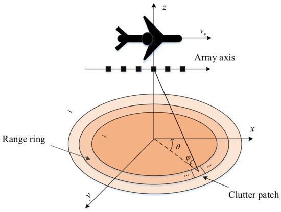
Figure 1.
Geometric configuration of an airborne surveillance radar.
Based on the Ward clutter model [36], the ground can be divided into distinct range rings, and each iso-range ring can be viewed as a superposition of a large number of discrete and mutually uncorrelated clutter patches. According to the geometry of the platform shown in Figure 1, the normalized Doppler frequency and normalized spatial frequency of the ith clutter patch can be defined as follows:
where and denote the elevation angle and azimuth angle, respectively.
Without considering the impact of range ambiguities, a clutter plus noise snapshot from a given iso-range ring then can be modeled as
where n is the thermal noise and is modeled as a zero-mean complex Gaussian vector with the covariance matrix ; Nc stands for the number of clutter patches; and denotes the complex amplitude and the space-time steering vector of ith clutter patch, which can be expressed as
Here and are the corresponding temporal and spatial steering vectors.
Since we suppose that the clutter patches are independent, the corresponding ideal clutter plus noise covariance matrix (CNCM) can then be written as
Based on the linearly-constrained minimum variance (LCMV) criterion, the optimum STAP weight vector can be obtained as
where denotes the target space-time steering vector.
In reality, the ideal CNCM is unknown and can be estimated by the maximum likelihood method from the IID adjacent range cells, i.e., , where is the number of available IID training samples. Due to the heterogeneous environment, it is often difficult to find adequate training samples, resulting in degraded clutter suppression performance.
2.2. SR-STAP Problem Formulation
The sparsity nature of the clutter spectra shows that only a small area is occupied by clutter on the entire space-time plane [18], which is exploited to estimate CNCM by sparse recovery techniques. For the SR-STAP algorithms [35], the continuous space-time plane is uniformly discretized into grids, where and are the number of grids in the spatial and temporal domain, and are the resolution scales. Then the SR-STAP signal model of the received clutter plus noise echoes from L range cells can be reformulated as
where is defined as an overcomplete dictionary matrix composed of the space-time steering vectors of grids, denotes the space-time profile matrix where each nonzero row stands for a potential clutter component, and is the noise matrix.
Since , it is an ill-posed problem to recover A using the ordinary least square method. Assuming the unknown profile A has row sparsity, i.e., the distribution of the non-zero elements is identical for each column of A. Then exploiting the sparsity nature of A, the sparse space-time profile can be acquired by solving the following mixed norm optimization problem [21]:
where is a nonnegative regularization parameter for balancing the row sparsity with data fidelity. This problem can be viewed as an norm penalized least-square estimator, also termed LASSO [37]. However, the convergence of LASSO cannot be guaranteed. In [23], Zou improved the LASSO by using a series of data-dependent weights to penalize different coefficients in the space-time profile instead of a common parameter , and the proposed the adaptive LASSO is given as:
where is the ith row of the space-time profile A, and denotes the weight of . Once the estimated space-time profile A is obtained, the corresponding CNCM can be recovered from
3. Proposed Algorithms
In this section, we first derive a complex-value adaptive Laplace-prior-based SBL STAP algorithm for the MMV case (i.e., CALM-SBL-STAP). Then an efficient localized reduced-dimension sparse recovery (LRDSR) processing scheme is developed to enhance the computational efficiency of CALM-SBL-STAP.
3.1. CALM-SBL-STAP Algorithm
From the Bayesian perspective, all of the unknown variables are considered random variables assigned to different distributions according to their priors. Similar to the other SBL models, we begin with the conventional assumption that the noise is modeled as white complex Gaussian with unknown power ; thus, we have:
where is the inverse noise variance, with a Gamma prior assigned on it as follows:
and the Gamma distribution is defined as [32]
where and represent the shape parameter and scale parameter, respectively, and denotes the ‘gamma function’. The mean and variance of x are respectively given as and .
Therefore, the Gaussian likelihood function of the measurements can be expressed as:
Since under the assumption of Gaussian noise, the observed likelihood function is not conjugate to the adaptive Laplace prior, and hence it cannot be used directly. To formulate the Bayesian model with adaptive Laplace priors, a hierarchical framework will be modeled for the unknown space-time profile A. We suppose each column of the sparse space-time profile is assigned with a zero-mean complex Gaussian prior as the first stage of the hierarchical model.
where is the variance for different rows in , and is a diagonal matrix with as the diagonal elements, i.e., . Further, in the second stage of the model, independent Gamma priors with parameter are placed on each in for the complex-value space-time signal model [38].
where .
Finally, based on the conjugate prior principle, a Gamma prior is assigned to
Figure 2 summarizes the probabilistic graphic model of the proposed complex hierarchical Bayesian model to illustrate the aforementioned hyperparameters. Combining the first two stages of the hierarchical Bayesian model (17) and (18), we can obtain the marginal probability distribution by integrating out :
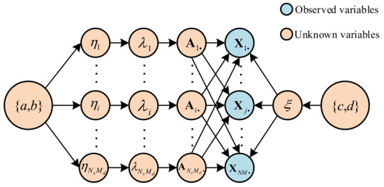
Figure 2.
Graphical model of the proposed hierarchical Bayesian model with complex adaptive Laplace prior.
It can be seen from (20) that the probability density function is a joint Laplace distribution with zero location parameters and different scale parameters. Each coefficient in the space-time profile is controlled by an independent hyperparameter , corresponding to the adaptive LASSO problem in (11) with the relationship [39].
Although the hierarchical model with an adaptive Laplace prior would be more complicated, the Laplace log-distribution has a sharper concave peak than Gaussian, allocating mass more on the axes so that the space-time profile is much preferred to close zero [28], as shown in Figure 3. Therefore, the Laplace distribution enforces the sparsity more heavily than a conventional Gaussian distribution. Meanwhile, the unimodal log distribution helps eliminate local minima. The modeling process of the proposed hierarchical Bayesian model in this article is motivated by [32,38], and we extend the real-value sparse recovery problem to STAP complex-value circumstance.
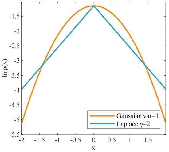
Figure 3.
Gaussian and Laplace log-distributions.
In the following, the expectation-maximization (EM) algorithm [29] is utilized for Bayesian inference to estimate the hyperparameters. The EM algorithm is an iterative framework for parameter estimation, alternating between the expectation step (E−step) and maximization step (M−step).
As widely known, based on the Bayesian theorem, the posterior probability can be calculated by
We can find that the posterior distribution is a multivariate Gaussian distribution with parameters
In E-step, the expectation of the logarithm of the joint distribution can be expressed as:
To update and , (24) can be simplified by omitting the irrelevant terms and according to (17)–(19), can be obtained as
In M-step, we can find the updates of and by maximizing (25) with respect to and separately. Next, the partial derivative of with respect to is:
where is the ith row of , is the (i, i)-th element of . However, directly solving (26) results in a slow convergence speed for the update of , inspired by [40,41], we establish a new fixed-point update rule to speed up the convergence.
Let , then (26) can be rewritten as
Analogously, the partial derivative of with respect to is:
Setting (27) and (28) to zero, the update rules of and can be respectively expressed as:
The logarithm function of noise precision in E-step can be expressed as:
Setting , we can find the update rule of :
It is worth noting that directly using (23) will result in a heavy computational burden. Fortunately, only the diagonal elements of are utilized during the process of updating the hyperparameters. Thus, in order to speed up the computation and save hardware storage space, we only need to calculate the diagonal elements [41].
The iteration operations alternate between E-step and M-step until a predefined stop criterion is satisfied. The pseudocode of the proposed algorithm (CALM-SBL-STAP) is shown in Algorithm 1.
| Algorithm 1 Pseudocode for CALM-SBL-STAP algorithm |
| Input: training samples X, dictionary matrix . Initialize: , , , . Set , . Step 1: While ; Update and using (22) and (33); Update using (29); Update using (30); Update using (32); If break end end Step 2: Estimate the CNCM by Step 3: Compute the space-time adaptive weight by (8) Step 4: Give the output of the CALM-SBL-STAP is |
3.2. LRDSR-STAP Scheme
Although various numerical experiments have proved that SBL algorithms can achieve favorable performance with only a few training samples, however, from (22) and (23), we can observe that it takes a costly O((NM)3) operations for matrix inversion at each iteration. Moreover, modern airborne radars often have hundreds or even thousands of system degrees of freedom, making them difficult to be implemented in real-time processing applications. Furthermore, conventional sparse-recovery algorithms need to search the entire space-time plane, and the overcomplete dictionary needs to be considerably dense to ensure the recovery accuracy, which also causes a heavy computational burden during each iteration.
To overcome these drawbacks, a novel localized reduced-dimension sparse-recovery-based space-time adaptive processing (LRDSR-STAP) method is proposed. Intuitively, to reduce the computational complexity, we can divide the existing SR-STAP problems into smaller problems to solve. If we divide the space-time plane into several regions along the Doppler frequency axis, the clutter in each localized area will still be sparsely distributed and can be recovered. Modern airborne pulse-Doppler radar systems can easily implement Doppler filter banks with extremely low sidelobes. Inspired by the formulations and properties of the PRI-staggered post-Doppler framework described in [6], deeply weighted Doppler filter banks can be utilized to acquire the narrow band localized clutter. Therefore, the received snapshots are firstly processed by K sliding window Doppler filters, for the mth Doppler bin,
where is an matrix whose columns represent the mth Doppler bin for the sliding window Doppler filters, and , here is the length of the sliding window, and is the temporal tapering window.
After filtering, the transformed clutter steering vector can be expressed as a reduced-dimension space-time steering vector .
where and are and temporal steering vectors respectively. Then (34) can be replaced with
where denotes the filtered amplitude.
In this structure, the localized clutter subspace can be estimated by steering vectors, where denotes rounding-up and represents the slope of clutter ridge, which is also the number of independent clutter observations [6]. Thus, it is proved that the localized reduced-dimension clutter is still low rank and can be sparsely recovered in the localized search region. At this time, only the grids within the mainlobe of the Doppler filter are required to form the dictionary and represent the localized clutter, as shown in the gray grids in Figure 4.
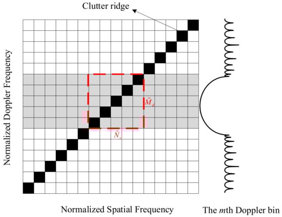
Figure 4.
Illustration of local grids selecting.
To further narrow the search region and improve the computational efficiency of sparse recovery, we present a knowledge-aided localized dictionary construction strategy. First, we can approximately estimate the slope of clutter ridge β using the prior knowledge provided by the inertial navigation system and radar system. A more refined localized dictionary is next assembled by the grids adjacent to the localized clutter ridge. As presented in Figure 4, for the mth Doppler bin, the grids in the dashed line are selected. Obviously, with the aid of prior knowledge, the size of the localized dictionary would be further reduced. Note that the size of the rectangular window is determined by the mainlobe width Δf of the Doppler filters and corresponding coupled spatial frequency range, i.e., only the grids within the spatial-temporal frequency range of fd,l∈[fm − Δf/2, fm + Δf/2] and fs,n∈[fm − Δf/2, fm + Δf/2]/β are selected, where fm is the central frequency of the mth Doppler bin. Finally, a prestored mask matrix Ξm is built to remove the redundant grids from the original dictionary Φ.
In this way, an even smaller localized reduced-dimension dictionary of mth Doppler bin is generated as
Now the reduced-dimension signal model in the case of multiple measurements can be rewritten as
where is the localized space-time profile matrix, which can be estimated by solving the following optimization:
Equation (41) is a standard adaptive LASSO optimization problem and can be solved by the previously proposed CALM-SBL algorithm. Obviously, this LRDSR-STAP processing scheme can scale down the CALM-SBL to a localized reduced-dimension region (the dimension of the dictionary and the signal are both reduced) hence the running speed of the CALM-SBL algorithm would be efficiently improved with the LRDSR processing scheme as a matter of course. We will refer to it as LRDSR-CALM-SBL in the following content. Figure 5 illustrates the processing block diagram of the proposed scheme. Since the size of the optimization problem decreases, the computational complexity of LRDSR-CALM-SBL in updating the hyperparameters and computing the STAP weights shrinks substantially.
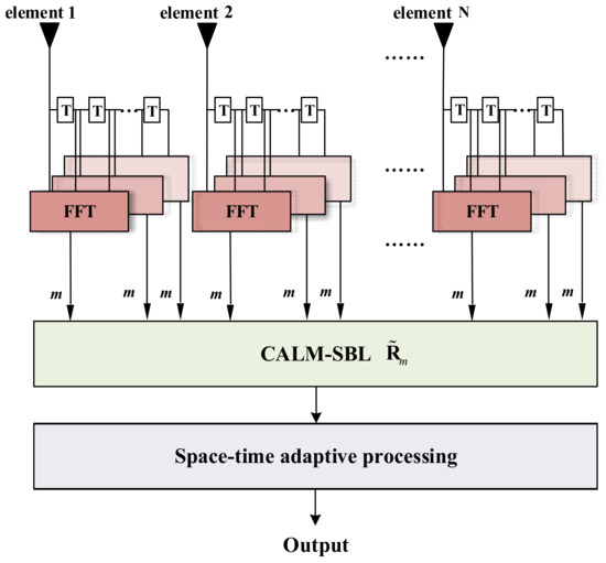
Figure 5.
Block diagram for LRDSR-CALM-SBL.
4. Numerical Simulation
In this section, extensive experiments are performed to assess the performance of the proposed algorithms (referred to as CALM-SBL and LRDSR-CALM-SBL) and compared with other existing methods. Unless otherwise specified, we consider a side-looking ULA with the following parameters: , , , , and . The simulated data are generated by the Ward clutter model mentioned in Section 2, and each range bin has clutter patches evenly distributed in azimuth angles. The clutter to noise ratio CNR = 50 dB, and noise power is set to be unitary, i.e., . The dictionary resolution scales are both set as , and the number of IID training samples L is 10. The prior parameters , , , and are set to a small value: . For fairness, we set the iteration tolerance and the maximum iterations for the proposed algorithms, M-SBL and M-FCSBL. To achieve the desired localized clutter spectrum, an 80-dB Chebyshev window is applied for the proposed LRDSR-CALM-SBL. Furthermore, all of the simulation results are averaged over 100 independent Monte-Carlo trails.
4.1. Computational Complexity Analysis
In the first experiment, we analyze the computational complexity of the proposed CALM-SBL and LRDSR-CALM-SBL for a single iteration and compare them with the other SR-STAP algorithms, including M-CVX [42], M-OMP [43,44], M-FOCUSS [45], M-SBL [29], and M-FCSBL [30]. The computational complexity is measured by the number of complex multiplications. For simplicity, the low-order terms of complex multiplications are omitted. The results are listed in Table 1, where denotes the clutter rank.

Table 1.
Computational complexity comparison.
As can be seen from Table 1, since only the diagonal elements are updated in (33), the computational complexity of CALM-SBL is moderately reduced and is lower than M-SBL. Because of the fact that and , the computational efficiency of the CALM-SBL has been significantly improved with the help of the proposed LRDSR-STAP processing scheme. Meanwhile, LRDSR-STAP performs dimensionality reduction in the time domain, so the heavy burden of matrix inversion is greatly reduced to during the process of calculating the space-time adaptive weight vector.
In order to present the comparison results more intuitively, the average code running time of these algorithms is examined, as shown in Table 2. Note that all the simulations are operated on the same platform with Intel Xeon 4114 CPU @2.2GHz and 128GB RAM. It can be seen from Table 2 that the average running time of the proposed LRDSR-CALM-SBL is greatly reduced compared to the original CALM-SBL and is much lower than M-SBL and M-FCSBL. The running time of LRDSR-CALM-SBL is even close to M-OMP and is already less than M-OMP when K = 1. In the subsequent experiments, we will also find that the proposed algorithms can maintain a satisfactory clutter suppression performance on this basis. This superiority makes LRDSR-CALM-SBL more suitable for practical real-time processing applications. Furthermore, this LRDSR processing scheme enables further parallel acceleration via multi-core processors (i.e., GPU), which is beyond the scope of the current paper.
Table 2.
Average running time comparison.
4.2. Clutter Suppression Performance
Due to the fact that LRDSR-CALM-SBL belongs to the reduced-dimension STAP algorithm, this means that it is essentially a suboptimal STAP method and will inevitably suffer from slight performance degradation compared with full-dimension STAP methods. Therefore, for the sake of fairness, we will separately compare the performance of CALM-SBL with other full-dimension STAP methods and LRDSR-CALM-SBL with other reduced-dimension STAP methods in our experiments.
Then we evaluate the clutter suppression performance via the metric of signal-to-interference-plus-noise (SINR) loss under various circumstances, which is defined as [21]:
where is the STAP weight vector, and is the clairvoyant CNCM.
Next, we first evaluate the SINR loss performance of CALM-SBL. Moreover, M-OMP, M-FOCUSS, M-SBL, M-FCSBL, and the optimum STAP are used as benchmarks. Note that M-CVX is not discussed here due to its overwhelming computational complexity. Figure 6 depicts the curves of the SINR loss versus the normalized Doppler frequency. As illustrated in Figure 6, all three SBL algorithms can similarly achieve near-optimum performance even with 10 training samples, and the proposed CALM-SBL consumes the least running time among these three algorithms.
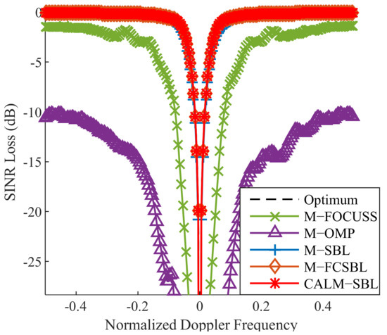
Figure 6.
SINR loss comparison of different SR-STAP methods.
Furthermore, in order to reveal the convergence speed of the proposed CALM-SBL, Figure 7 presents the average SINR loss with different numbers of training samples. The average SINR loss is defined as the mean of the SINR loss values for . It is indicated that the average SINR of all methods increases with the increment of training samples. Apparently, the proposed algorithm exhibits a fast convergence speed similar to the other two SBL algorithms and achieves a near-optimum performance with merely two training samples, attributed to the fact that the adaptive Laplace prior facilitates a sparser solution.
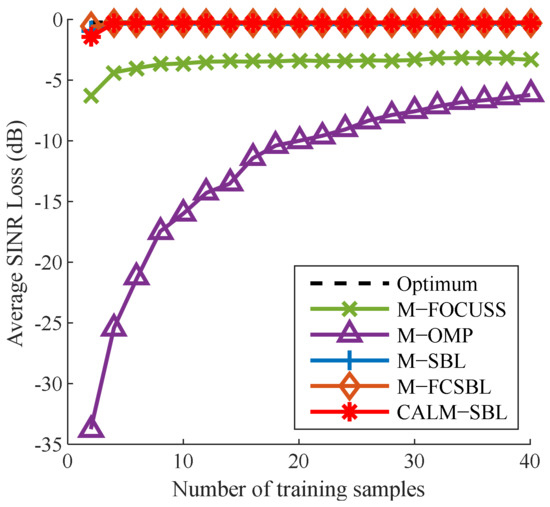
Figure 7.
The average SINR loss against the number of samples.
From the above full-dimension STAP experiments, we can observe that the proposed CALM-SBL has a satisfactory performance. However, in the current practical engineering applications, the full-dimensional STAP is still difficult to be implemented due to the limitation of processor capability, and thus the reduced-dimension processing scheme is more preferred. Therefore, in the following experiments, we will mainly focus on comparing the proposed LRDSR-CALM-SBL with other RD-STAP methods.
Figure 8 demonstrates the SINR loss performance of the proposed LRDSR-CALM-SBL algorithm with different K. It can be observed that the notch of K = 1, the simplest form, is much wider than others. This is because adaptive processing is only performed in the spatial domain at this time. With the increase of K, the available space-time adaptivity increase, and the clutter suppression performance is also improved with a narrower notch. Based on our empirical study, K = 3 generally leads to satisfactory performance. Considering the balance of performance and efficiency, we will employ K = 3 in the subsequent experiments.
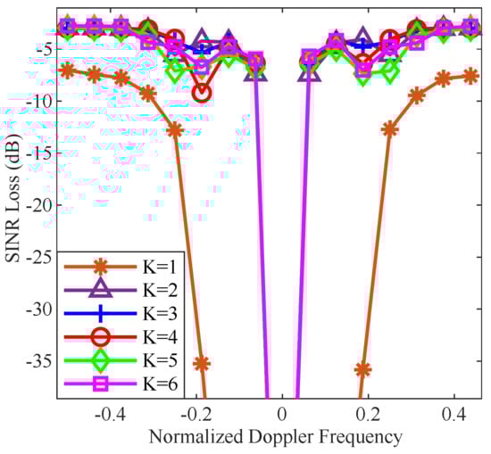
Figure 8.
SINR loss comparison of different K.
In the next experiment, we compare the SINR loss performance with other RD methods, such as a state-of-the-art RDSR algorithm [34], and conventional statistic RD-STAP algorithms with diagonal loaded to the noise power level, such as the PRI-staggered post-Doppler [6] with three sliding windows, the direct data domain (DDD) [14] with subaperture, the joint-domain localized (JDL) [5] with beam-Doppler channels, and the optimum full-dimensional STAP. Furthermore, four typical cases, as presented in Figure 9, are considered: (a) the ideal case; (b) the spatial mismatch case in the presence of gain-phase error; (c) the temporal mismatch case in the presence of the intrinsic clutter motion (ICM); (d) the ideal case when β = 0.5. From Figure 9a, the curves show that the two reduced-dimension SR-based methods outperform the conventional methods and can obtain satisfying performance in a heterogeneous environment. Specifically, the RDSR exhibits a wider notch, and thus the proposed method has a superior minimum detectable velocity (MDV) performance. It can be observed from Figure 9b that all the SR-STAP methods suffer performance loss due to the model mismatch between the dictionary and clutter data. In Figure 9c, the proposed method shows a decreased performance compared to the ideal case since ICM leads to a broadened clutter spectrum, where more space-time vectors are needed to represent the clutter. In Figure 9d, when β = 0.5, all the SR methods encounter the off-grid effect and have a degraded performance.
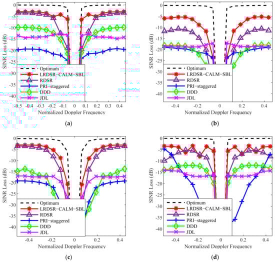
Figure 9.
SINR loss comparison of different RD-STAP methods in four different cases. (a) Ideal case. (b) Spatial mismatch case. (c) Temporal mismatch case. (d) Ideal case when β = 0.5.
In Figure 10, we evaluate the average SINR loss compared to a different number of training samples , i.e., the convergence rate. The average SINR loss is also defined as the mean of the SINR loss values for . As demonstrated in Figure 10, the curve of the LRDSR-CALM-SBL has a 3.5 dB improvement over the curve achieved by RDSR. Therefore, the proposed method can obtain superior performance even with insufficient sample support and exhibits a faster convergence speed than the other considered algorithms.
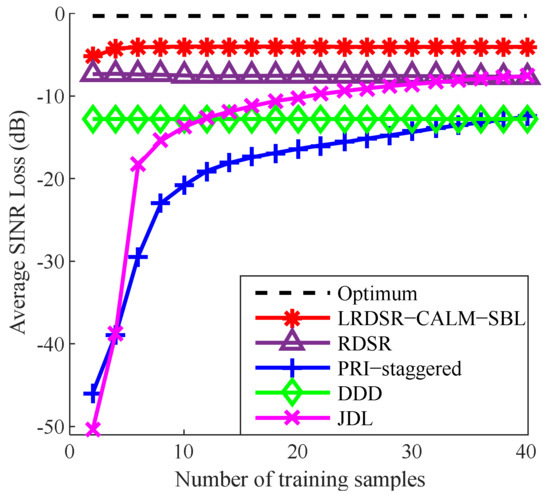
Figure 10.
The average SINR loss against the number of samples.
Finally, we verify the target detection performance improvement via the probability of detection () versus the target SNR curves acquired by employing the cell-averaging CFAR (CA-CFAR) detector [46]. One hundred targets are assumed in the boresight and randomly injected into the whole Range-Doppler plane. The probability of a false alarm rate is next set to be 10−3, and the related detection threshold is obtained by estimating the noise floor from the data surrounding the CUT. As illustrated in Figure 11, there exist over 1 dB SNR improvement when the is 0.8. In general, the proposed algorithm shows better detection performance than other compared methods.
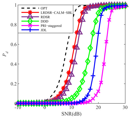
Figure 11.
Probability of detection versus target SNR.
5. Discussion
This research aims to develop an effective and efficient STAP algorithm for airborne radar with insufficient training samples in inhomogeneous environments.
Based on the quantitative and qualitative analysis from the previous Sections. A hierarchical structure is employed to build the sparse Bayesian learning model with adaptive Laplace priors. Compared with the existing Gaussian prior [29,30], it can promote the sparsity more heavily and ensure a higher recovery accuracy. It can be seen from Figure 6 that the proposed CALM-SBL is closer to the optimal STAP performance than the Gaussian-prior-based M-SBL algorithm, as summarized in Table 3.
Table 3.
SINR loss comparison of Figure 6.
In addition, although the average SINR loss of the CALM-SBL is not as good as that of M-SBL when there are only two training samples, as the number of samples increases, the performance will outperform that of M-SBL, as shown in Table 4.
Table 4.
The average SINR loss comparison of Figure 7.
Similar to other SBL algorithms, large-scale matrix inversion operation and several large-scale matrix calculations are involved in each iteration process, resulting in high computational complexity, especially when the radar system has a high space-time degree of freedom. Benefiting from the fact that we only update the diagonal elements in the process of updating , as detailed in Equation (33), the average running time of CALM-SBL is 10.1729 s, while that of M-SBL and M-FCSBL are 288.9466 s and 40.8802 s, respectively. Moreover, we next propose the LRDSR processing scheme to accelerate CALM-SBL by scaling down the CALM-SBL to a localized reduced-dimension region. After the computational complexity analysis in Table 1 and the comparison of average code running time in Table 2, we can observe that LRDSR-CALM-SBL only takes about one percent of the running time of the original CALM-SBL when K = 3. It should be noted that the LRDSR is essentially a reduced-dimension STAP processing scheme and inevitably suffers a certain performance loss [36]. Table 5 evaluates the SINR loss performance of CALM-SBL in Figure 6 and LRDSR-CALM-SBL in Figure 9a. As shown in Table 5, the SINR loss performance is about 3–4 dB lower. Although there is certain performance degradation, its running speed has been significantly improved, which is an acceptable trade-off in practical engineering applications.
Table 5.
SINR loss comparison of CALM-SBL and LRDSR-CALM-SBL.
6. Conclusions
In this work, we firstly developed a complex adaptive Laplace-prior-based SBL STAP algorithm by introducing an improved hierarchical Bayesian model to endow the hyperparameters with a complex Laplace prior, thus obtaining a superior performance than an SBL algorithms with a Gaussian prior in a sample shortage case. To decrease the computational requirements of the proposed CALM-SBL, especially in the context of a high-dimensional modern radar system, an efficient localized reduced-dimension sparse-recovery-based STAP processing scheme is then investigated. By exploiting the local sparsity and prior knowledhtte of the clutter, a localized reduced-dimension dictionary is constructed, and the computational efficiency is considerably enhanced. All of the simulation results have illustrated that the proposed methods overcome the limitation of the training samples and alleviate the influence of the computational complexity on the real-time processing system.
Author Contributions
Conceptualization, W.C. and T.W.; investigation, D.W.; methodology, W.C. and D.W.; project administration, T.W.; software, W.C.; supervision, K.L.; visualization, W.C.; writing—original draft, W.C.; writing—review & editing, K.L. All authors have read and agreed to the published version of the manuscript.
Funding
This research was funded by National Key R&D Program of China, grant number 2021YFA1000400.
Conflicts of Interest
The authors declare no conflict of interest.
References
- Brennan, L.E.; Mallett, J.D.; Reed, I.S. Theory of Adaptive Radar. IEEE Trans. Aerosp. Electron. Syst. 1973, 9, 237–251. [Google Scholar] [CrossRef]
- Klemm, R. Principles of Space-Time Adaptive Processing; The Institution of Electrical Engineers: London, UK, 2002. [Google Scholar]
- Guerci, J.R. Space-Time Adaptive Processing for Radar; Artech House: Norwood, MA, USA, 2003. [Google Scholar]
- Reed, I.S.; Mallett, J.D.; Brennan, L.E. Rapid Convergence Rate in Adaptive Arrays. IEEE Trans. Aerosp. Electron. Syst. 1974, 10, 853–863. [Google Scholar] [CrossRef]
- Wang, H.; Cai, L. On adaptive spatial-temporal processing for airborne surveillance radar systems. IEEE Trans. Aerosp. Electron. Syst. 1994, 30, 660–670. [Google Scholar] [CrossRef]
- Ward, J.; Steinhardt, A.O. Multiwindow Post-Doppler Space-Time Adaptive Processing. In Proceedings of the IEEE Seventh SP Workshop on Statistical Signal and Array Processing, Quebec, QC, Canada, 26–29 June 1994. [Google Scholar]
- Wang, Y.L.; Chen, J.W.; Bao, Z.; Peng, Y.N. Robust space-time adaptive processing for airborne radar in nonhomogeneous clutter environments. IEEE Trans. Aerosp. Electron. Syst. 2003, 39, 70–81. [Google Scholar] [CrossRef]
- Shi, J.X.; Xie, L.; Cheng, Z.Y.; He, Z.S.; Zhang, W. Angle-Doppler Channel Selection Method for Reduced-Dimension STAP Based on Sequential Convex Programming. IEEE Commun. Lett. 2021, 25, 3080–3084. [Google Scholar] [CrossRef]
- Goldstein, J.S.; Reed, I.S. Reduced-rank adaptive filtering. IEEE Trans. Signal Process. 1997, 45, 492–496. [Google Scholar] [CrossRef]
- Goldstein, J.S.; Reed, I.S. Theory of partially adaptive radar. IEEE Trans. Aerosp. Electron. Syst. 1997, 33, 1309–1325. [Google Scholar] [CrossRef]
- Haimovich, A.M. The eigencanceler: Adaptive radar by eigenanalysis methods. IEEE Trans. Aerosp. Electron. Syst. 1996, 32, 532–542. [Google Scholar] [CrossRef]
- Ayoub, T.F.; Haimovich, A.M.; Pugh, M.L. Reduced-rank STAP for high PRF radar. IEEE Trans. Aerosp. Electron. Syst. 1999, 35, 953–962. [Google Scholar] [CrossRef]
- Wang, Y.L.; Liu, W.J.; Xie, W.C.; Zhao, Y.J. Reduced-rank space-time adaptive detection for airborne radar. Sci. China Inf. Sci. 2014, 57, 1–11. [Google Scholar] [CrossRef]
- Sarkar, T.K.; Wang, H.; Park, S.; Adve, R.; Koh, J.; Kim, K.; Zhang, Y.H.; Wicks, M.C.; Brown, R.D. A deterministic least-squares approach to space-time adaptive processing (STAP). IEEE Trans. Antennnas Propagat. 2001, 49, 91–103. [Google Scholar] [CrossRef] [Green Version]
- Melvin, W.L.; Showman, G.A. An approach to knowledge-aided covariance estimation. IEEE Trans. Aerosp. Electron. Syst. 2006, 42, 1021–1042. [Google Scholar] [CrossRef]
- Wicks, M.C.; Rangaswamy, M.; Adve, R.; Hale, T.B. Space–time adaptive processing: A knowledge-based perspective for airborne radar. IEEE Signal Process. Mag. 2006, 23, 51–65. [Google Scholar] [CrossRef]
- Maria, S.; Fuchs, J. Application of the Global Matched Filter to Stap Data an Efficient Algorithmic Approach. In Proceedings of the 2006 IEEE International Conference on Acoustics Speech and Signal Processing, Toulouse, France, 14–19 May 2006. [Google Scholar]
- Yang, Z.C.; Li, X.; Wang, H.Q.; Jiang, W.D. On Clutter Sparsity Analysis in Space-Time Adaptive Processing Airborne Radar. IEEE Geosci. Remote Sens. Lett. 2013, 10, 1214–1218. [Google Scholar] [CrossRef]
- Zhang, W.; He, Z.S.; Li, H.Y. Space time adaptive processing based on sparse recovery and clutter reconstructing. IET Radar Sonar Navig. 2019, 13, 789–794. [Google Scholar] [CrossRef]
- Sun, K.; Meng, H.; Wang, Y.; Wang, X. Direct data domain STAP using sparse representation of clutter spectrum. Signal Process. 2011, 91, 2222–2236. [Google Scholar] [CrossRef] [Green Version]
- Sun, K.; Zhang, H.; Li, G.; Meng, H.; Wang, X. A novel STAP algorithm using sparse recovery technique. In Proceedings of the 2009 IEEE International Geoscience and Remote Sensing Symposium, Cape Town, South Africa, 12–17 July 2009. [Google Scholar]
- Fan, J.; Li, R. Variable Selection via Nonconcave Penalized Likelihood and Its Oracle Properties. J. Am. Stat. Assoc. 2001, 96, 1348–1360. [Google Scholar] [CrossRef]
- Zou, H. Adaptive lasso and its oracle properties. J. Am. Stat. Assoc. 2006, 101, 1418–1429. [Google Scholar] [CrossRef] [Green Version]
- Kanitscheider, I.; Coen-Cagli, R.; Pouget, A. Origin of information-limiting noise correlations. Proc. Natl. Acad. Sci. USA 2015, 112, 6973–6982. [Google Scholar] [CrossRef] [Green Version]
- Pregowska, A. Signal Fluctuations and the Information Transmission Rates in Binary Communication Channels. Entropy 2021, 23, 92. [Google Scholar] [CrossRef]
- Zhang, M.L.; Qu, H.; Xie, X.R.; Kurths, J. Supervised learning in spiking neural networks with noise-threshold. Neurocomputing 2017, 219, 333–349. [Google Scholar] [CrossRef] [Green Version]
- Wang, Y.; Xu, H.; Li, D.; Wang, R.; Jin, C.; Yin, X.; Gao, S.; Mu, Q.; Xuan, L.; Cao, Z. Performance analysis of an adaptive optics system for free-space optics communication through atmospheric turbulence. Sci. Rep. 2018, 8, 1124. [Google Scholar] [CrossRef]
- Tipping, M.E. Sparse Bayesian learning and the relevance vector machine. J. Mach. Learn. 2001, 1, 211–244. [Google Scholar]
- Duan, K.Q.; Wang, Z.T.; Xie, W.C.; Chen, H.; Wang, Y.L. Sparsity-based STAP algorithm with multiple measurement vectors via sparse Bayesian learning strategy for airborne radar. IET Signal Process. 2017, 11, 544–553. [Google Scholar] [CrossRef]
- Wang, Z.T.; Xie, W.C.; Duan, K.Q.; Wang, Y.L. Clutter suppression algorithm based on fast converging sparse Bayesian learning for airborne radar. Signal Process. 2017, 130, 159–168. [Google Scholar] [CrossRef]
- Liu, K.; Wang, T.; Wu, J.; Chen, J. A Two-Stage STAP Method Based on Fine Doppler Localization and Sparse Bayesian Learning in the Presence of Arbitrary Array Errors. Sensors 2022, 22, 77. [Google Scholar] [CrossRef]
- Babacan, S.D.; Molina, R.; Katsaggelos, A.K. Bayesian Compressive Sensing Using Laplace Priors. IEEE Trans. Image Process. 2010, 19, 53–63. [Google Scholar] [CrossRef]
- Han, S.D.; Fan, C.Y.; Huang, X.T. A Novel STAP Based on Spectrum-Aided Reduced-Dimension Clutter Sparse Recovery. IEEE Geosci. Remote Sens. Lett. 2017, 14, 213–217. [Google Scholar] [CrossRef]
- Guo, Y.D.; Liao, G.S.; Feng, W.K. Sparse Representation Based Algorithm for Airborne Radar in Beam-Space Post-Doppler Reduced-Dimension Space-Time Adaptive Processing. IEEE Access 2017, 5, 5896–5903. [Google Scholar] [CrossRef]
- Li, Z.Y.; Wang, T.; Su, Y.Y. A fast and gridless STAP algorithm based on mixed-norm minimisation and the alternating direction method of multipliers. IET Radar Sonar Navig. 2021, 15, 1340–1352. [Google Scholar] [CrossRef]
- Ward, J. Space-Time Adaptive Processing for Airborne Radar; Lincoln Laboratory: Lexington, MA, USA, 1994. [Google Scholar]
- Maleki, A.; Anitori, L.; Yang, Z.; Baraniuk, R.G. Asymptotic analysis of complex LASSO via complex approximate message passing (CAMP). IEEE Trans. Inf. Theory 2013, 59, 4290–4308. [Google Scholar] [CrossRef] [Green Version]
- Pedersen, N.L.; Manchón, C.N.; Badiu, M.A. Sparse estimation using Bayesian hierarchical prior modeling for real and complex linear models. Signal Process. 2015, 115, 92–109. [Google Scholar] [CrossRef] [Green Version]
- Themelis, K.E.; Rontogiannis, A.A.; Koutroumbas, K.D. A novel hierarchical Bayesian approach for sparse semisupervised hyperspectral unmixing. IEEE Trans. Signal Process. 2012, 60, 585–599. [Google Scholar] [CrossRef]
- Wipf, D.P.; Rao, B.D. An empirical Bayesian strategy for solving the simultaneous sparse approximation problem. IEEE Trans. Signal Process. 2007, 55, 3704–3716. [Google Scholar] [CrossRef]
- Wang, Q.; Yu, H.; Li, J.; Chen, F. Sparse Bayesian Learning Using Generalized Double Pareto Prior for DOA Estimation. IEEE Signal Process. Lett. 2021, 28, 1744–1748. [Google Scholar] [CrossRef]
- Grant, M.; Boyd, S. CVX: Matlab Software for Disciplined Convex Programing, Version 2.0 Beta. Available online: http://cvxr.com/cvx (accessed on 14 September 2013).
- Tropp, J.A. Greed is good: Algorithmic results for sparse approximation. IEEE Trans. Inf. Theory 2004, 50, 2231–2242. [Google Scholar] [CrossRef] [Green Version]
- Tropp, J.A. Algorithms for simultaneous sparse approximation, part II: Convex relaxation. Signal Process. 2006, 86, 589–602. [Google Scholar] [CrossRef]
- Cotter, S.F.; Rao, B.D.; Engan, K.; Kreutz-Delgado, K. Sparse solutions to linear inverse problems with multiple measurement vectors. IEEE Trans. Signal Process. 2005, 53, 2477–2488. [Google Scholar] [CrossRef]
- Liu, W.J.; Liu, J.; Hao, C.P.; Gao, Y.C.; Wang, Y.L. Multichannel adaptive signal detection: Basic theory and literature review. Sci. China Inf. Sci. 2022, 65, 121301. [Google Scholar] [CrossRef]
Publisher’s Note: MDPI stays neutral with regard to jurisdictional claims in published maps and institutional affiliations. |
© 2022 by the authors. Licensee MDPI, Basel, Switzerland. This article is an open access article distributed under the terms and conditions of the Creative Commons Attribution (CC BY) license (https://creativecommons.org/licenses/by/4.0/).