Abstract
Plant phenotyping plays an important role for the thorough assessment of plant traits such as growth, development, and physiological processes with the target of achieving higher crop yields by the proper crop management. The assessment can be done by utilizing two- and three-dimensional image reconstructions of the inhomogeneities. The quality of the reconstructed image is required to maintain a high accuracy and a good resolution, and it is desirable to reconstruct the images with the lowest possible noise. In this work, an electrical impedance tomography (EIT) data acquisition system is developed for the reconstruction and evaluation of the inhomogeneities by utilizing a non-destructive method. A high-precision EIT system is developed by designing an electrode array sensor using a cylindrical domain for the measurements in different planes. Different edible plant slices along with multiple plant roots are taken in the EIT domain to assess and calibrate the system, and their reconstructed results are evaluated by utilizing an impedance imaging technique. A non-invasive imaging is carried out in multiple frequencies by utilizing a difference method of reconstruction. The performance and accuracy of the EIT system are evaluated by measuring impedances between 1 and 100 kHz using a low-cost and rapid electrical impedance spectroscopy (EIS) tool connected to the sensor. A finite element method (FEM) modeling is utilized for image reconstruction, which is carried out using electrical impedance and diffuse optical tomography reconstruction software (EIDORS). The reconstruction is made successfully with the optimized results obtained using Gauss–Newton (GN) algorithms.
1. Introduction
EIT is an imaging method that can estimate the electrical impedance distribution inside an object. The EIT sensor system consists of an electrode array with a single or multiple layers, and the current density is distributed inside the medium based on the stimulated current through the electrodes [1,2,3]. A small current is injected into the object’s surface through a pair of electrodes and then the impedance distribution and the corresponding conductivity are estimated. Electrical resistivity or conductivity images of any closed domain under test can be reconstructed using the boundary potentials [1,2]. The data obtained by measuring all possible impedances are used to reconstruct an image, which may provide qualitative and quantitative information.
EIT could provide a cost-effective alternative to the established imaging methods across a wide range of applications. EIT has a high temporal resolution, but it has a poor spatial resolution, so this technique is sensitive to noise. Although the spatial resolution of EIT is less than magnetic resonance imaging (MRI), EIT is easy to use and its cost is much less than the cost of MRI, which can make EIT a useful screening tool for imaging. The spatial resolution can be improved by increasing the number of electrodes in the EIT system and by choosing the correct drive pattern upon the selection of electrode pairs for current and voltage stimulation [4,5]. Due to its unique advantages, EIT has enormous applications in biomedical imaging, plant physiology, biotechnology, nanotechnology, and material engineering. EIT is becoming popular in research, offering exceptionally good benefits of non-invasive, non-ionizing, fast imaging speed, and low-cost monitoring. From the images of EIT, the physiological information of the matter can be obtained that can be used for real-time applications [5,6].
Multifrequency EIT (MFEIT) systems give more useful information about biological matters because the electrical voltage appearing across the matter is frequency dependent [7,8,9,10]. Significant information about the matters can be obtained by injecting currents in multiple frequencies and measuring the impedances at different electrode positions. A good conductivity distribution of an object can be mapped in the domain under test by measuring the electrical impedances through the multiple electrodes at various frequencies. The image of an object can be reconstructed by calculating the boundary voltages in homogeneous and inhomogeneous conditions of the domain under test and with the help of finite element method (FEM) modeling [2,8]. In EIT, the FEM technique is used to derive the forward model from the governing equation, which is described by Laplace’s equation [1,2,5]. In forward solve, the boundary potentials are calculated by the injected current and known conductivity distribution inside the EIT domain. On the other hand, the unknown conductivity changes are calculated in the inverse solve by knowing the differences in boundary potentials of two different media for the given stimulation current in the domain.
A multifrequency impedance imaging technique can be utilized considering a multi-electrode array with eight or more electrodes in a domain for obtaining the more useful information of an inhomogeneity. The EIS method was applied in the electrode array system, and the reconstructed images were presented in multiple frequencies by the phantom experiments [11]. Therefore, EIT is a non-invasive, and non-destructive impedance imaging technique. It is a radiation-free, rapid, and cost-effective alternative to other laboratory-based imaging methods such as MRI, computed tomography (CT), and positron emission tomography (PET). The estimation performance can be potentially improved by considering a multispectral impedance imaging technique using an EIT system [7,9]. Due to its unique advantages, EIT has enormous applications in cell imaging [6], brain imaging [12], anomaly detection [13,14], and crop root imaging [15,16,17,18], respectively.
Previously, EIT image reconstruction was made considering different algorithms in multiple works [8,19,20,21,22]. An FPGA-based data acquisition system at 1–190 kHz was developed considering 16 electrodes for two-dimensional (2D) brain imaging by Shi et al. [12]. Two-dimensional imaging, characterization, and monitoring of oilseed plant root systems were made at frequencies of 0.46 Hz–45 kHz considering an array of 38 electrodes by Weigand and Kemna [15,16]. A rapid estimation of wheat plant root biomass by measuring capacitance up to 20 kHz using a handheld LCR meter was proposed by Postic et al. [17]. The development of oilseed plant root was visualized using a data acquisition system in three-dimensions (3D) at frequencies of 5–10 kHz considering an array of 32 electrodes by Corona-Lopez et al. [18]. The methods of all these works required expensive instrumentations and most of them were found as laboratory-based and not suitable for in situ measurements. In addition, several data acquisition systems based on EIT were developed for industrial and medical applications and those were utilized for different previous research works on clinical imaging [10], health monitoring [23], and diagnosis of human body diseases with anomaly detection [24]. The outputs of these EIT systems were limited to 2D imaging. Hence, a portable and high-speed multifrequency 3D EIT data acquisition system for in situ applications in plant phenotyping is still a constant requirement.
The characterization in phenotyping refers to qualitative and quantitative descriptions of the plant’s biological characteristics, such as morphological, physiological, and biochemical. Identifying the size, shape, and structure of the roots or other bodies of the plant, growth, and development with the event of photosynthesis, and quantifying the chemical properties such as water and nutrients are very important in biological study of the plant characteristics. The root system of a plant plays an important role in photosynthesis by which the water and nutrients are transferred to the plant stems and leaves by absorbing from soil. The flowering plants are classified as vascular (reproduced by seeds/vegetative parts), which contain a specialized xylem and phloem tissues for the transportation of water and nutrients, while the non-flowering plants are classified as non-vascular (reproduced by spores), which do not contain specialized vascular tissues for transport.
An investigation on growth, development, and biomass of the root is very important for characterization in plant phenotyping. The investigation can be made by varying the electrical parameters such as, capacitance, resistance, or impedance. In several experiments, the dependency of electrical impedance on plant characteristics was found and evaluated at different frequencies [11,15,16,18]. An imaging method was utilized to characterize the root by measuring the electrical parameters. Previously, based on the electrical parameters, the root biomass was estimated by Postic et al. [17], analysis on root growth was made by Ozier-Lafontaine et al. [25], and the root body of a plant in water was recovered by Liao et al. [26]. The imaging of water distribution in the root zone was made in a laboratory-scale rhizotron container in a soil media and recovered 2D information only by Newill et al. [27]. More information on root structure, density, and distributions can be obtained by utilizing a 3D imaging system, which is advantageous over 2D. Spectral variations on root characteristics can be made using a 3D imaging system. The growth and development of the root can be monitored precisely by knowing the electrical characteristics in multiple frequencies obtained using a 3D EIT system. Presently, Weigand and Kemna utilized a multifrequency EIT system in a laboratory for root characterization and imaging in a water-filled rhizotron considering polarization effects and recovered 2D information only [15,16], Corona-Lopez et al. visualized the developing root system in a compost-filled container using multifrequency EIT and recovered some 3D information of the root at a low frequency of 5 kHz; no information was found about the high spectral performance [18].
In addition, the changes on root characteristics during growth can be evaluated by employing the measurements considering frequency-difference and time-difference EIT [7,8,14,28]. Image reconstruction using difference data at two injecting frequencies at a particular time, or the data obtained for single frequency measurements over a time duration can be made successfully using a 3D imaging system. A new cost-effective and high spectral range 3D EIT system along with the existing measurement methods is still a constant requirement in the field of root study. Non-invasive imaging using 3D, monitoring growth, and estimating biomass at the laboratory and field scale are still demanding. EIT using a portable multiple electrode array with capability of 3D imaging seems to be a promising method to fulfill the scope of further research on plant phenotyping.
In this work, a rapid, low-cost, and high-precision EIT data acquisition system is developed with the target of applications in plant phenotyping for the non-destructive evaluation of the inhomogeneities considering a non-invasive impedance imaging technique in multiple frequencies.
2. Materials and Methods
2.1. Design of EIT Electrode Array Sensor System
A cylindrical plastic domain of 4.5-inch diameter, 3-inch height, and 0.0625-inch thickness was taken. An EIT electrode array of sixteen metal electrodes was designed and the electrodes were configured in two layers (eight electrodes each) of the domain as shown in Figure 1b. The electrodes were with one-half inch diameter, one inch per arm length (L shaped electrodes with two arms), and 0.0625-inch thickness. The electrode arrangement in the layers is aligned. The bottom layer consisted of eight electrodes that were placed equally 1.25 inches apart and at a 1.25-inch top from the bottom position by keeping 0.25-inch separation of the electrodes from the base of the domain as shown in Figure 1a. Another eight electrodes of same size are placed similarly in another layer at a 0.75-inch top position from the bottom layer as shown in Figure 1b.
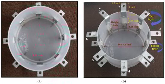
Figure 1.
An electrode array sensor with (a) 8 electrodes (bottom layer) for 2D EIT, and (b) 16 electrodes (top and bottom layers) designed in a cylindrical domain for 3D EIT measurements.
The size of the domain, number, and location of electrodes in a layer, and type and dimensions of the electrodes were optimized by conducting several experiments considering previous research works [10,29,30]. Steel electrodes were chosen, which were found comparatively less expensive than the other electrodes made by highly conductive materials such as silver, copper, or aluminium. The chosen electrodes were silver-colored electroplates made of zinc-plated steel material. The electrodes were found suitable with good current carrying capability and with a good correlation between the measured impedances and dimensions (length and diameter) of the electrodes. The electrodes were numbered sequentially in the domain of EIT sensor system. After designing, the sensor was tested and characterized by the injected current. The measurements were carried out considering 8 metal electrodes for 2D and 16 metal electrodes for 3D. A good conductivity distribution was found with the optimized dimensions of the electrodes and the electrode array system was found suitable for 3D EIT imaging by the measurements considering a planar-aligned electrode placement configuration [30]. The electrodes were placed vertically in the same line of the domain and found an optimal design as shown in Figure 1b. A low-cost EIT sensor was able to be designed and the measurement method with this arrangement was found robust in obtaining tomography of a sample with less noise and less error.
2.2. Development of EIT Data Acquisition System
An automated EIT data acquisition system is developed for the measurements considering 2D and 3D operations, as shown in Figure 2. An EIS tool EVAL-AD5933EBZ was interfaced with Arduino Uno (ATmega328P), EIS data storage (PuTTY), and electrode switching multiplexers (CD74HC4067). AD5933 is a high-precision impedance converter system that combines an on-board frequency generator; it has programmable graphic user interface with frequency sweep capability and serial I2C interface [31,32,33]. The EIT sensor is connected to the EIS tool through multiplexers. Two multiplexers were connected with EIT electrode array system for 2D or 3D operations by injecting currents and capturing boundary voltages. The impedance of an object in the domain was measured by the current injected through the electrodes with an automated and appropriate EIS measurement settings using Arduino Uno programming. The measured impedances for all the electrodes in a 2D/3D system were stored by varying frequencies and output excitations controlled by the EIS tool (AD5933). In addition, a 15 MHz DDS signal generator (JDS6600) was used to obtain the current carrying capability of the electrodes. The current is injected in different frequencies through the driving electrodes and the AC sensing voltages were measured for different current levels by the sensing electrodes using a multimeter. The data were stored using the acquisition systems and analyzed for EIT image reconstruction in MATLAB using an open-source software, EIDORS [2,10,11,23].
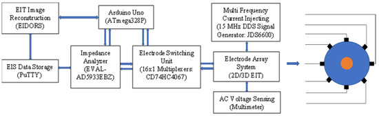
Figure 2.
A developed EIT data acquisition system for 2D and 3D imaging.
2.3. Calculating Conductivity
The physical relationship between the conductivity and the boundary voltages in the domain is governed by a partial differential equation that is derived from Maxwell’s equations. To obtain the conductivity, the EIT inverse solution is required and, hence, the forward problem is solved at first. The boundary voltage is calculated for the given conductivity distribution and the injected current. In this work, a complete electrode model is used and EIT problems are solved numerically by utilizing FEM modeling.
In the EIT experiment, a small mA current is injected through an electrode array with L = 8 or 16 electrodes at frequencies 1–100 kHz, and the boundary voltages are measured. When current Il is injected through electrode el on the surface . and the conductivity distribution is known, the electric potential V in the domain can be solved from the governing equation with the boundary conditions for the complete electrode model.
According to KCL, in the absence of independent electric charges, the summation of the outward and inward current at any point of a closed surface inside the domain is zero,
According to Ohm’s law, the relation between the current density () and the electric field () is
With quasi-static assumption, the electric field can be written in the form of a gradient of a scalar potential (V) as
In the continuum electrode model, there are no electrodes facing the boundary of an object. The model assumes that the current density is a continuous function on the entire boundary of the object. Comparing the Equations (1)–(3), the sensing field (EIT governing equation) can be described by Laplace’s equation (derived from Maxwell’s equation) [1,2,5] as follows:
The gap model assumes the discrete electrodes on the surface of an object, and the shunting effect of the electrodes and contact impedance is ignored. Consider, the current is injected in the boundary through discrete electrodes, thus, the current density Jl is injected through the l-th electrode is given in [1,5] by
This must be satisfied in the boundary, where is considered as the outward unit normal vector.
The shunt model refines the gap model by taking into account the shunting effect of the electrode. The current is injected in the boundary through the electrodes and calculated using Neumann boundary condition [1,5] as
The complete electrode model is a refinement of the shunt electrode model in which the shunting effect and contact impedance between the electrodes and the object in the medium is taken into account. The measured voltage on electrode el is which is given by the Dirichlet boundary condition [1,5] as
where Zl is the effective contact impedance between the electrode and the object in the medium.
The injected current and the measured voltages are also satisfied as , and . The optimum conductivity distribution is calculated by the voltage difference, , where Vh and Vi are the measured voltages in homogeneous and inhomogeneous media. The conductivity map of the inhomogeneity in a single step can be calculated using [1,5,12] as follows:
where J is the Jacobian, which is a determinant for the measurement of voltage sensitivity, W is the inverse of the covariance of measurements, R is an estimation of the inverse of the noise covariance, and λ is the hyperparameter that controls the trade-off between resolution and noise attenuation in the reconstructed image.
2.4. FEM Modeling
EIT problems were solved numerically with the help of finite element method (FEM) modeling. An EIT ‘distmesh’ model of ‘d2d4c’ with 8 electrodes using the ‘mk_common_model’ was optimized for the designed electrode array system in the 2D domain as shown in Figure 3a. The model consisted of 2507 numbers of nodes, 4757 numbers of elements, and 255 numbers of boundaries. On the other hand, a ‘Netgen’ cylindrical model using ‘ng_mk_cyl_models’ was optimized for modeling in the 3D domain with 16 electrodes distributed in two layers (8 electrodes in each layer), as shown in Figure 3b. The model consisted of 3247 numbers of nodes, 13,963 numbers of elements, and 3264 numbers of boundaries, respectively. The effects of variations of nodes, elements, and boundary numbers on the reconstruction results were examined thoroughly. An optimization was made by employing different boundary conditions and a satisfactory result was obtained using the selected models.
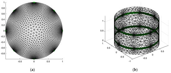
Figure 3.
FEM Models for (a) d2d4c: 2D (circular) with 8 electrodes, and (b) Netgen: 3D (cylindrical) with 16 electrodes EIT.
The FEM modeling was carried out using EIDORS, whose operation was made with the help of MATLAB for the reconstruction using the EIT measurements. EIS data were stored using an open-source software PuTTY (interfaced with Arduino Uno COM3 port) and a statistical analysis was performed. The flowchart of the EIDORS operation is presented in Figure 4. The sensing methods were applied, and the conductivity of the inhomogeneous object was mapped with the following steps: (i) 2D/3D FEM model selection, (ii) stimulation, (iii) forward solve: homogeneous and inhomogeneous data loading, and (iv) inverse solve: reconstruction of the inhomogeneity by the conductivity calculations using one-step Gauss–Newton (GN) algorithms such as prior NOSER, Gaussian HPF, Laplacian, and Tikhonov regularization. The optimized controlling parameters such as the size of the domain, the inhomogeneity position and size, the stimulation current/voltage (I/V), the frequency (f), and the hyperparameter value (λ) were set for the measurements and stimulation, and the overall reconstruction performance was made accordingly.
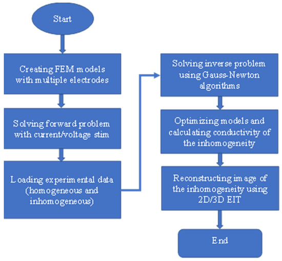
Figure 4.
Flowchart of EIDORS operation.
The common EIT inverse algorithms for FEM modeling are Gauss–Newton (GN), Shefield back-projection (BP), and total variation (TV), respectively [10,19,34]. The GN method is an iterative algorithm to solve nonlinear least squares problems, BP is a linear reconstruction algorithm, and TV is a regularization-based algorithm. Electrical impedance imaging is a highly nonlinear and ill posed inverse problem in which a minimization algorithm is used to obtain its approximate solution [10,19].
The objective function can be minimized by taking the difference between the experimental measured data and the predicted data. If Vm is the measured voltage matrix and Vc is the calculated voltage matrix, then the Gauss–Newton (GN) algorithm gives a least square solution of the minimized object function s(σ) [2], which is defined as
Back-projection (BP) is capable of producing images of changes in conductivity. The images produced by BP have some clear artifacts because of the inherent character of the asteroid trace and the conductivity is given by
where L is the number of electrodes, Vm is the measured voltage, p is the position of electrodes, and J is the current density function.
The back-projection algorithm is known to blur image contrasts. Reconstruction using a total variation (TV) functional helps to preserve discontinuities in reconstructed profiles, which are smoothened by traditional reconstruction algorithms such as Newton’s algorithm. Edge-preserving algorithms such as those using TV are more complex to implement in addition to the high computational cost. The TV of a conductivity image is defined as
where Ω is the region to be imaged. Since the conductivity is constant over each FEM element, is non-zero only on the edges between elements. For the i-th edge, shared by the FEM elements m(i) and n(i), the jump in conductivity is: . The variation over the complete image can be found by integrating the jump over all the edges of the mesh as
where li is the length of i-th edge in the mesh, and the index i covers all the edges.
Several machine learning algorithms such as an artificial neural network (ANN), a least angle regression (LARS), and an elastic net were also studied previously for EIT inverse solution [35,36,37]. A classic deterministic Gauss–Newton with Laplacian regularization method were compared with the machine learning algorithms [35]. A good reconstruction was made using the modified ANN compared to the modified LARS and elastic net. ANN suffers from long training and reconstruction times; LARS and elastic net seem to be less accurate for real time data but much faster than ANN [35]. Most of the algorithms have some limitations in obtaining 3D images, among these the Gause–Newton method was found faster in training and computation and suitable for 3D image reconstruction with high accuracy.
2.5. Experimental Setup and Sensor Characterization
An EIT experimental setup for the data acquisition is presented as shown in Figure 5. The sensing methods applied to the EIT sensor were optimized and utilized based on the requirements considering homogeneous and inhomogeneous conditions. The results were validated, and the methods were found suitable in obtaining good reconstruction performance. An automated and high-speed data acquisition for multiple samples such as edible plant slices, and plant roots in the domain was possible in a short duration by utilizing the AD5933 EIS tool. Finally, a difference method was applied for the obtained datasets and the reconstructed results of the inhomogeneities were obtained by varying the stimulation current in 2D and 3D planes.
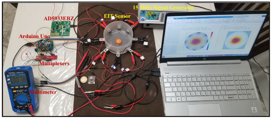
Figure 5.
An EIT experimental setup for image reconstruction of the inhomogeneities. The data were stored by the measurements using EIS tool and DDS signal generator. For example, a carrot slice was placed at the centre of the domain and that was reconstructed using EIDORS.
Initially, the EIS sensor using AD5933 was characterized, and the functionality of the tool was tested by measuring impedances of a carrot slice of height 1/5-inch and diameter, D = 25.4 mm to utilize in the EIT data acquisition system. The EIS measurements of the sample were carried out using two-pole method by varying the output excitation (Vout) and spacing between two electrodes. A pair of electrocardiograms (ECG) electrodes connected to AD5933 was separated by d distance and the reactance, Xc of a sample was calculated as , and sample capacitance, , where A is the cross-sectional area and ε is the medium constant. The electrical impedance (Z) of a sample measured by the EIS tool (AD5933EBZ) is related to the DFT magnitude of and gain factor [32,33] as follows:
where the gain factor is calibrated by a known resistance of 7.5 kΩ. The gain factor varies with the variation of output excitation and physical frequency (f) for a given sample. Here, re and im are the DFT real and imaginary outputs registered at different frequency codes generated by the physical frequency, , where fclk is the master clock frequency of 16.776 MHz for the internal oscillation [32].
The sample reactive (X) and resistive (R) components are calculated as . and , where phase of the electrical impedance, , and Z is the magnitude of the impedance. The influence of impedance magnitude in determining the sample characteristics was found much higher than the phase. Hence, the impedance magnitude obtained from AD5933 was taken for a different analysis of the experiments. The sample characteristics can be determined by obtaining the impedance spectroscopy in a wide range of frequencies. The EIS characteristics of the samples were obtained by varying frequencies up to 100 kHz controlled by the EIS tool.
To study the EIS characteristics, the output excitation was varied from 0.4 to 2 Vpp and the spacing between two electrodes was varied from 0.3 to 1.5 cm, as shown in Figure 6. As a result, the impedance was decreased with the increase in excitation, on the other hand, the impedance was increased with the increase in the separation of the electrodes. More than a 95% correlation was found, and the impedance profile indicated a good conductivity distribution with the optimized output excitation of 2 Vpp and 1 cm spacing of the electrodes.
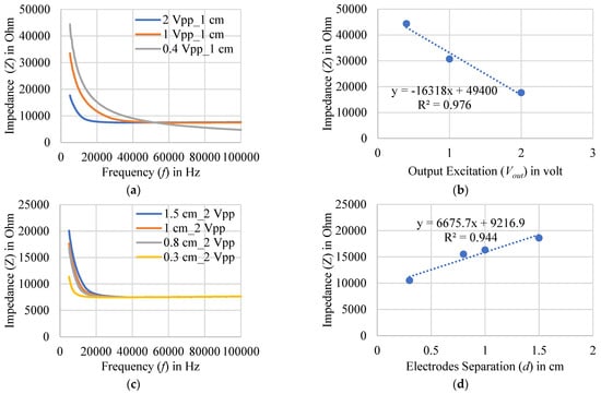
Figure 6.
EIS measurements of a carrot slice using two-electrode method (a) by varying output excitation, and (b) the corresponding correlation. EIS measurements (c) by varying separation of the electrodes, and (d) the corresponding correlation. A good correlation with more than 95% coefficient was found for the measurements using 2 Vpp excitation and 1 cm spacing of the electrodes.
In this work, two approaches were taken for the measurements in homogeneous and inhomogeneous media of the EIT domain. The EIT domain was filled with water to create the homogeneous media. A continuous signal of 2 Vpp excitation was applied to the EIT sensor system, and the measurements were carried out. At first, a two-pole method was applied, and EIS measurements were carried out using an EVAL-AD5933EBZ impedance analyzer. The impedances for different layers of electrodes in the domain were obtained for different frequencies of 1–100 kHz. A total of 64 measurements (1-1, 1-2, 1-3, 1-4, 1-5, 1-6, 1-7, and 1-8 with respect to electrode 1; 2-1, 2-2, 2-3, 2-4, 2-5, 2-6, 2-7, and 2-8 with respect to electrode 2, and so on) were taken from the eight-electrode system in one layer for 2D. In addition, the measurements were taken in other layers of the sensor electrode array for 3D. A constant current source of 1 mA sinusoidal current with varying frequency was found suitable for EIT [10,11,23]. The current is injected through the electrodes of the array and the obtained boundary voltages for a single layer of the EIT sensor are depicted in Figure 7.
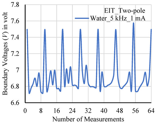
Figure 7.
The boundary voltages for a homogeneous media (water) at 5 kHz, and 1 mA signal considering two-pole measurements in one layer of EIT domain.
In addition, a four-pole method was utilized for obtaining the reconstruction results at multiple frequencies up to 100 kHz considering a 1 mA or above sinusoidal current. The current was injected through the driving electrodes using a 15 MHz DDS signal generator at different frequencies and the voltages were measured through the sensing electrodes. The signal responses for 5 kHz and 1 mA are depicted as shown in Figure 8. In the 1st projection, the current (I) was applied through neighboring electrodes 1-2 and five differential voltages (V1, V2, V3, V4, and V5) were measured between 3-4, 4-5, 5-6, 6-7, and 7-8 electrode pairs. In the 2nd projection, the current was injected through 2-3 electrodes and the differential voltages (V1–V5) were collected from 4-5, 5-6, 6-7, 7-8, and 8-1 electrode pairs. Thus, for the eight current projections a total of L(L-3) = 8 × 5 = 40 voltage measurements were taken from a L = 8 electrode EIT system. The highest current density was found in the driving electrodes and that decreases with the distance. Hence, the voltage was low at the opposite sensing electrodes position from the current-driven electrodes. The variation of the voltages was observed sinusoid as shown in Figure 8a.
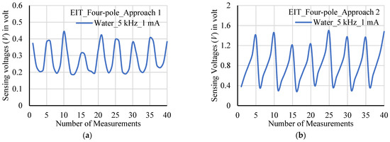
Figure 8.
The sensing voltages for a homogeneous media (water) at 5 kHz and 1 mA signal considering four-pole measurements with (a) 1st approach, and (b) 2nd approach in one layer of EIT domain.
In another approach using the four-pole method, the current through neighboring electrodes 1–2 and five differential voltages (V1-V5) were measured between 3-4, 3-5, 3-6, 3-7, and 3-8 electrode pairs. Next, the current was driven through 2-3 electrodes and the voltages (V1-V5) were measured between 4-5, 4-6, 4-7, 4-8, and 4-1 electrode pairs. In the similar way 40 voltage measurements were taken for the eight electrode EIT system. The measured voltage in the sensing electrodes was increased with the increase in distance when moving towards clockwise, and the results are presented in Figure 8b.
The carrot sample was then placed in the EIT domain filled with water. The impedances of the inhomogeneous media (water + carrot) were measured by the designed electrode system in the bottom layer of the array by varying the output excitation from 0.4 to 2 Vpp at 5, and 80 kHz, respectively. A two-pole method was applied for the measurements using the designed multi-electrode sensor. The impedance was decreased by increasing frequency and output excitation as well as shown in Figure 9. The effect of output excitation may vary based on the size of the electrodes, electrodes spacing, signal frequency, and type of the samples placed in the domain. A large oscillation with high impedance was observed for a low output excitation of 0.4 Vpp, where the gain and DFT outputs oscillated highly for a given frequency. The results were found stable at a 2 Vpp excitation where a good conductivity of the sample was found, and all the experiments were made accordingly with this high excitation. The suitability of the electrode system was found by the sensor characterization using AD5933. In a similar way, the other samples were taken in the measurements. Later, the boundary potentials were calculated using forward solve and a good reconstruction was made by the calculated conductivity.
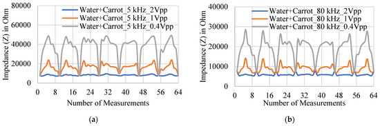
Figure 9.
EIS measurements for an inhomogeneous media (water + carrot) in the domain consisting of eight electrodes by varying output excitation at (a) 5 kHz, and (b) 80 kHz, respectively.
The boundary voltages were calculated for different stimulation currents by measuring impedances in homogeneous (water) and inhomogeneous (water with sample) media, and the difference of those was used to map the conductivity of the sample in the domain. The voltages were normalized to obtain the conductivity of the sample. The effects of impedances of electrodes and wires/clips were minimized accordingly, and a good tomographic result of the sample was obtained. The voltage distributions using two-pole sensing method was found more stable and uniform. The measured boundary data played an important role in obtaining tomography and using the two-pole method the impedances of the electrodes were found very sensitive to the measurements for the taken objects in the EIT domain.
3. Results
The designed electrode array system was tested considering multiple inhomogeneities in the domain and the reconstruction was made in 2D and 3D planes in different experiments. The dimensional and frequency dependency of different plant roots were examined considering 3D image reconstruction.
3.1. Image Reconstruction in 2D Plane
Experiment 1: In an experiment, the impedances were measured for a carrot slice (height, h = 1/5-inch, and diameter, D = 25.4 mm) in a cylindrical domain using an EIT electrode array system. The impedances were varied for different frequencies of 5–100 kHz with the output excitation of 2 Vpp. A good conductivity distribution was found, and the image reconstruction was carried out by placing the carrot slice at different positions (pos: centre, 1, 4, and 7) in the domain. The results were reconstructed successfully using a ‘d2d4c’ FEM model for 80 kHz and a 1 mA stimulation current considering GN: Laplace (λ = 0.57) in the inverse model as shown in Figure 10. The maximum change of conductivity was found higher (0.725 S/m or above) at the side wall than the centre (0.61 S/m) of the domain because the maximum current passes through the side wall.
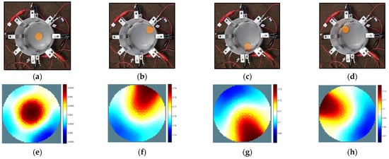
Figure 10.
A carrot slice at different positions of (a) pos: centre, (b) pos: 1, (c) pos: 4, and (d) pos: 7 in the EIT domain. (e–h) The corresponding reconstructed images for 80 kHz, 1 mA, and Laplace (λ = 0.57). The obtained conductivity is high at the side wall, and it is low at the centre.
Further, the stimulation current was varied for a domain with a carrot slice at position 1 and the new reconstructed results were obtained as shown in Figure 11. The conductivity was increased from 0.77 to 0.85 S/m with the increase in current from 0.5 to 2 mA for a constant hyperparameter value of λ = 0.57. The reconstructed results were also obtained by varying hyperparameter values of 0.97, 0.57, and 0.17, respectively, at 1 mA for a domain with a carrot slice at position 7 as shown in Figure 12. The conductivity was increased from 0.71 to 0.9 S/m with the decrease in the hyperparameter value.
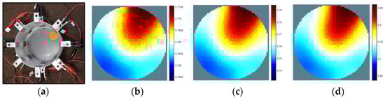
Figure 11.
A carrot slice at (a) pos: 1, and the reconstructed images for the stimulation current of (b) 0.5 mA, (c) 1 mA, and (d) 2 mA at 80 kHz considering GN: Laplace (λ = 0.57). The shape of the inhomogeneity changes with the increase in current (a slight change is observed). The conductivity is increased, and the obtained maximum conductivity values are 0.77, 0.79, and 0.85 S/m, respectively.
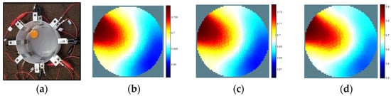
Figure 12.
A carrot slice at (a) pos: 7, and the reconstructed images for the hyperparameter value (λ) of (b) 0.97, (c) 0.57, and (d) 0.17 at 80 kHz and 1 mA considering Laplace algorithm. The shape of the inhomogeneity changes with the decrease in hyperparameter value. The conductivity is increased, and the obtained maximum conductivity values are 0.71, 0.73, and 0.9 S/m, respectively.
Experiment 2: In another experiment, three different edible plant slices of carrot, radish, and potato of a 1/3-inch height with a diameter, D = 25.4 mm of each were taken in the EIT domain and their reconstructed results were obtained using the impedance imaging technique in the 2D plane (using ‘d2d4c’), as shown in Figure 13. In this case, the overall size of all the plant slices were taken same. EIS measurements of the samples were carried out from 5 to 100 kHz. A total of 64 measurements were taken for both homogeneous and inhomogeneous conditions using 2 Vpp output excitation, and the difference was taken for the reconstruction of each plant slice for 1 mA stimulation current considering the GN: GHPF algorithm. Potato was found more conductive at a low frequency of 5 kHz and a good conductivity distribution of carrot was found at the high frequencies. At 5 kHz, the conductivity of the samples was obtained as 0.9, 1.1, and 3.6 S/m, respectively, considering the hyperparameter value of λ = 0.17. The sensing voltage increases with the increase in frequency and dimension as well and more useful information can be obtained from the sample. At 80 kHz, the conductivity of the carrot was increased to 2.8 S/m. An improved conductivity of carrot slice was found by increasing the height from 1/5-inch to 1/3-inch. The conductivity of the carrot was further increased to 9.1 S/m by increasing the stimulation current from 1 to 2 mA. Thus, the frequency, dimensions, and stimulation current played an important role in achieving a good conductivity distribution and in obtaining clear reconstructed images.
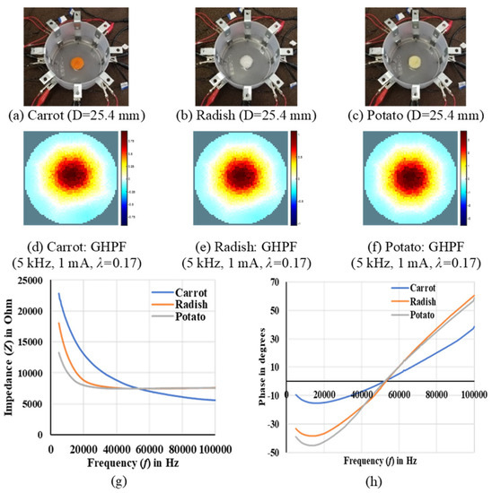
Figure 13.
(a–c) Different edible plant slices (carrot, radish, and potato) placed in bottom layer of electrodes of a cylindrical domain, (d–f) the corresponding reconstructed images, and (g,h) their impedance spectroscopy results. GHPF algorithm is utilized, and potato is found more conductive at 5 kHz, 1 mA, and 2 Vpp output excitation. In addition, the carrot sample has good conductivity distribution at the high frequencies.
Experiment 3: Later, multi-target anomalies such as bio-, conductive-, and non-conductive targets were considered in the designed EIT domain and simultaneous imaging was carried out using the different measurement techniques. The boundary voltages for multiple inhomogeneities such as metal, plastic, metal + plastic, and plastic + carrot in the domain were calculated by measuring impedances at different frequencies up to 100 kHz. A good reconstruction was made considering GN: GHPF with the optimized hyperparameter values for 5 kHz and 1 mA current and the results are presented as shown in Figure 14.
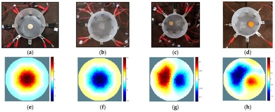
Figure 14.
(a) Metal, (b) Plastic, (c) Metal + Plastic, and (d) Plastic + Carrot inhomogeneities at the centre of the EIT domain. The corresponding reconstructed images are presented at 5 kHz and 1 mA considering GHPF and the hyperparameter value (λ) of (e) 0.17, (f) 0.17, (g) 0.17, and (h) 0.017, respectively. The type of inhomogeneity from the mixed is identified successfully with the optimized hyperparameter value.
The conductivity level varies depending on the position and type of inhomogeneity in the domain, and by varying the other controlling parameters. A good reconstruction was made using a ‘distmesh’ generator ‘d2d4c’ for a circular model. The inhomogeneities were identified successfully in the domain and the simultaneous two-dimensional imaging with a good accuracy was possible using the designed electrode array system. The metal and carrot are conductive, and the plastic is resistive. The metal has a higher conductivity than the carrot. The overall conductivity of the carrot was increased by decreasing the hyperparameter value (λ) and a clear reconstructed image was obtained. The multiple inhomogeneities with different electrical properties in the domain were able to distinguish using the developed EIT system.
3.2. Image Reconstruction in 3D Plane
Experiment 1: At first, the EIS measurements for a homogenous media considering water in a cylindrical domain was carried out at different frequencies of 5–100 kHz using the designed multi electrode sensor system. The measurements were also carried out for an inhomogeneous media considering water and a carrot (length: L = 3 inch, and diameter: D = 31.75 mm) with a biomass weight of W = 54 g in the given area of the domain. The carrot was considered as a sample of a tap root system. A total of 64 measurements were taken from the eight-electrode array system in the top layer. The variation of impedances was observed sinusoid for the measurements at different electrode positions. The impedance was decreased by increasing the frequency for a constant output voltage excitation of 2 Vpp and the results are presented for a homogeneous media, as shown in Figure 15a. The impedance distribution in the top layer considering an inhomogeneous media (water + carrot) is presented for 80 kHz and 2 Vpp excitation, as shown in Figure 15b.

Figure 15.
Impedance spectroscopy for (a) homogeneous (water), and (b) inhomogeneous (water + carrot) media in the top layer of the cylindrical domain at 2 Vpp output excitation. Impedance is decreased in different electrodes position by increasing frequency.
In addition, the EIS measurements were taken in the top to bottom and bottom layers of the electrode array in the domain by using an experimental set up as shown in Figure 16. The boundary voltages were calculated with impedance data obtained from homogeneous and inhomogeneous media of the EIT domain and those were normalized. A 3D reconstruction of the carrot (L = 3-inch, W = 54 g) was made by calculating the changes of conductivity from the difference of normalized voltages at an 80 kHz, 1 mA, and 2 Vpp output excitation as shown in Figure 16c. The prior NOSER algorithm performed well compared to the other inverse algorithms for 3D imaging and considered with the optimized hyperparameter value of λ = 2.17. The conductivity of the carrot was obtained considering the layers of electrodes at z = 1, and z = 0.3, respectively, with a virtual layer at z = 0.65 in the cylindrical FEM mesh. It was found that day wise (day 1 to 3) the biomass weight of the carrot sample was decreased from W = 54 g (L = 3 inch) to W = 34 g (L = 2.5 inch) at room temperature (20 °C) and the average impedance was increased at different frequencies, as shown in Figure 16b. The moisture level was reduced along with the dimension of the carrot and the corresponding tomography was distorted by decreasing the conductivity of the sample with time as shown in Figure 16d.
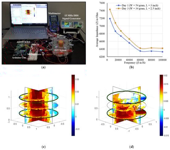
Figure 16.
(a) A 3D EIT experimental setup for obtaining impedance tomography of a carrot sample (tap root) in a cylindrical domain. (b) Average impedance profile of the sample by varying frequency in different days (day 1 and day 3). The reconstructed images of the sample obtained in (c) day 1, and (d) day 3 at 80 kHz, 1 mA, and 2 Vpp excitation considering GN: NOSER (λ = 2.17). The average impedance of the carrot is decreased with the increase in frequency and the impedance is increased at different frequencies with time. The maximum conductivity of the sample is decreased from 0.033 to 0.02 by reducing the biomass weight and dimension with time. It is found that biomass of a carrot has dimensional dependency.
Later, four different carrot samples of various biomass weights (W = 54, 88, 52, and 46 g) and dimensions (length, L = 3, 3.1, 2.75, and 2.8 inches with diameter of D = 31.75 mm each) were taken, and the correlation was established with the measured impedances. The layer-wise impedance distribution in a cylindrical domain was taken and the average impedances of the full model were correlated with fresh biomass weights and lengths of the carrots. At 5 kHz, more than an 85% correlation was found with weight and length of the carrots, as shown in Figure 17. The average impedance was decreased with the increase in weight and length of the carrot, and the carrot sample was found more conductive. In addition, an improved correlation of more than a 90% coefficient (R2 = 0.822) was found between the average impedance and biomass weight of the carrot at a high frequency of 60 kHz, where R2 is the coefficient of determination and R is the correlation coefficient. It indicates that the biomass of the carrot is dependent on not only the dimensions of the sample but also the frequencies of the signal.
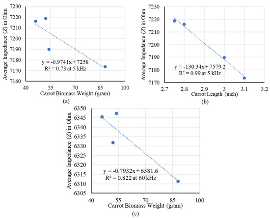
Figure 17.
Correlation between (a) average impedance and biomass weight, and (b) average impedance and length of the carrot at 5 kHz. A negative correlation is found between the carrot size (such as weight and length) and average impedance. An improved correlation is found between (c) average impedance and biomass weight of the sample at a high frequency of 60 kHz. Overall, the average impedance is decreased by increasing frequency and the correlation is improved for estimating the carrot root biomass.
Experiment 2: In an experiment, a potato plant was grown at room temperature as shown in Figure 18, and the root of the plant species was taken as one of the samples for the analysis of 3D image reconstruction using the developed EIT data acquisition system. The root structure, dimensions, and variation of frequencies were examined on obtaining the tomography result of the root by measuring the electrical impedances using the designed EIT sensor system. The length of the root was measured as 10 inches when the shoot length of the plant was 16 inches. In addition, the root system of the potato species is tap root, which includes an old seed piece. The potato root was placed in water media of the EIT domain for the measurements of impedances at room temperature (20 °C) and the reconstruction was made using the developed EIT system as shown in Figure 19a.
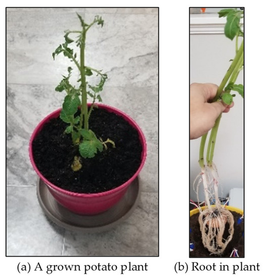
Figure 18.
(a) A grown potato plant, and (b) a potato root system in plant.
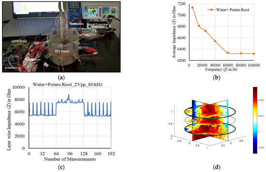
Figure 19.
(a) An EIT experimental setup for the measurements of a potato root system, (b) average measured impedances for 5–100 kHz of an inhomogeneous media (water + root), (c) layer-wise measured impedances at 80 kHz, and (d) reconstructed potato root (tap root) using 3D EIT measurements in water at 80 kHz, 2 Vpp, and 1 mA stimulation current considering GN: NOSER (λ = 2.17). The obtained result shows a conductive behaviour of the root with maximum changes of conductivity of 0.003.
The impedances were measured for homogeneous (water) and inhomogeneous (water + potato root) conditions by varying frequencies from 5 to 100 kHz using an EIS tool (AD5933) connected to the EIT sensor. The impedances were measured at a 2 Vpp excitation in different layers such as top, top to bottom, and bottom layers of the electrode array. The average impedances obtained for the inhomogeneous media are presented in Figure 19b and the impedances were found to decrease with the increase in frequency. Layers-wise, the measured impedances are presented in Figure 19c. The boundary voltages were calculated for a 1 mA stimulation current and normalized. The differences of the voltages were utilized to calculate the changes of conductivity for the given root system in the EIT domain, which represents the tomography. A tomography of the potato root system was made at 80 kHz and 1 mA using the difference method by applying the one-step GN algorithm: NOSER with the optimized hyperparameter value of 2.17 as shown in Figure 19d. A conductive behaviour of the root was found with the maximum changes of conductivity of 0.003 for the selected electrode positions at z = 1 and 0.3 vertically (including a virtual layer at z = 0.65) in the electrode array system. A tomography of the potato root system was made successfully using FEM modeling.
The fresh weight of the root was measured as 46 g when it was separated from the shoot of the plant. During the measurements, the root sample did not suffer any physical damage and was active in operation. Later, the root was kept in the free space at room temperature, the root was dried by removing the moisture, and day-wise the weight was measured. The biomass weight was reduced to less than 20 g in a week, where excluding the old seed, the actual root was found as 2 g only in dry condition. The several plants of the same can be taken in a further experiment for modeling the measured impedances with fresh or dry biomass weights of the roots.
Experiment 3: In another experiment, the root impedance of a Chinese money plant (Pilea) species was measured by placing the sample in the designed cylindrical EIT domain with the target of obtaining 3D reconstruction, as shown in Figure 20. The homogeneous media was created by filling the water in the domain and the measurements were taken without and with the root accordingly. The difference was used to calculate the root conductivity. The impedances for two different media were measured by the electrode layers of the domain using AD5933 from 5 to 100 kHz at room temperature (20 °C) and the corresponding boundary potentials were calculated at 1 mA. The changes of conductivity of the root were calculated by the differences of normalized boundary voltages.
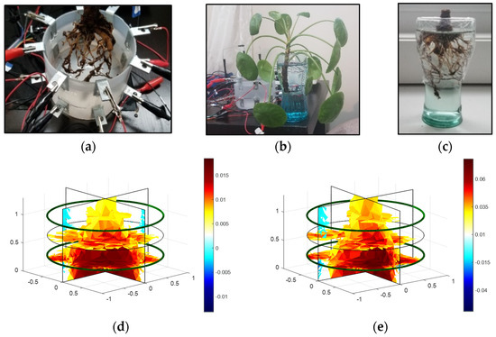
Figure 20.
3D imaging of a Pilea root in a cylindrical domain using EIT measurements and considering GN: NOSER inverse algorithm (λ = 2.17). (a) Measuring root impedance, (b) Chinese money plant (Pilea), (c) Pilea root, and the reconstructed root images at 1 mA for (d) 5 kHz (2 Vpp), and (e) 80 kHz (0.4 Vpp), respectively. An improved conductivity of the root was found by increasing the frequency.
The obtained tomography results are presented at 5 kHz (Vout = 2 Vpp), and 80 kHz (Vout = 0.4 Vpp), respectively. After optimizing, good results were found with the selected frequencies and excitations considering GN: NOSER (λ = 2.17) in the inverse model. The maximum changes of conductivity of 0.018 was obtained at 5 kHz and 2 Vpp, as shown in Figure 20d. The impedance with a low excitation of 0.4 Vpp was minimized by increasing the frequency to 80 kHz and the maximum changes of conductivity of the root was increased to 0.08, as shown in Figure 20e. As a result, the tomography of the root was made successfully using FEM modeling. The conductivity was varied at different vertical electrode positions of z = 1, and 0.3 including a virtual layer of z = 0.65. A higher conductivity is found at the bottom layer of the electrodes’ position where the impedance is low because of distributed roots. It is concluded that the impedance varies by the variation of root density and distribution of the roots, and the variations in tomography results are obtained accordingly.
The fresh weight of the root was measured as 90 g when it was separated from the plant. During the measurements, the root sample did not suffer any physical damage and was active in operation. Later, the EIS measurements of the Pilea root were carried out using two ECG electrodes connected to an EIS tool (AD5933) from 5 kHz to 100 kHz by varying the output excitation from 0.4 to 2 Vpp, as shown in Figure 21. The root impedance was increased with the increase in electrodes separation and a good positive correlation was found for 3 cm spacing. On the other hand, the root impedance was decreased with the increase in frequency and the output excitation as well. A small variation of the root impedances was found by varying the output excitation and the correlation was negative, as shown in Figure 21b. After optimizing, a good match was found with the selected spacing of the electrodes considering the output excitation of 2 Vpp, and more than a 94% correlation was found at 5 kHz.
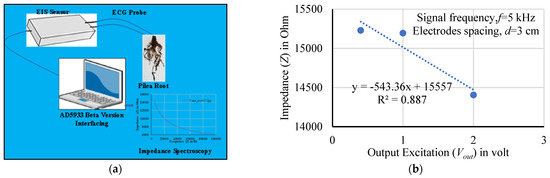
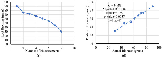
Figure 21.
(a) EIS measurement of a Pilea root using AD5933EBZ, and (b) the corresponding correlation with output excitation. (c) Day-wise the biomass of the root was decreased for different measurements, and the corresponding impedance was increased. (d) A good correlation with R2 = 0.983 and RMSE of 3.75 was obtained by the predicted model at 5–7 kHz considering 2 Vpp excitation.
The EIS measurements of the Pilea root were taken on different days and the results were correlated with the biomass weights. The impedances were found to increase by decreasing the biomass of the root. The moisture level of the root was reduced with time and, hence, the conductivity of the root was decreased. The biomass weight of the root was reduced from 90 to 30 g in three weeks at room temperature (20 °C) and those were predicted by the measured impedances. The regression analysis was performed using the measured root biomass and impedances obtained in 20 days when it was kept at free space. A good correlation with R2 = 0.983 and RMSE of 3.75 was found at 5–7 kHz considering n = 8 samples and selected features of k = 4 in the dataset, as shown in Figure 21d. A statistical analysis was performed with the obtained data using PrimaXL Data Analysis ToolPak [31,33]. A multiple linear regression analysis was performed for the obtained dataset considering the least square method [31,33] with the help of Equation (14).
where Zf1, Zf2, …., Zfk are the average impedances for k number of features of f1 to fk. The intercept is , and are the coefficients.
A dataset suffers from the multicollinearity problem: (i) if the correlation coefficient (R) between the explanatory variables is close to one, (ii) if there is no change in the coefficient of determination (R2) after adding an independent variable, and (iii) if the tolerance value (tolerance = 1 − R2) is less than 0.1 and the variance inflation factor (VIF = 1/tolerance) is greater than 10. At first, the highly correlated features of more than a 95% correlation coefficient were removed. Later, the Wrapper backward elimination method was applied considering the probability of rejection of the null hypothesis p ≤ 0.05 using an individual t-test. After few iterations, the training and validation was performed considering the overall F-test (p ≤ 0.05) and the features (5, 5.5, 6, and 7 kHz) were selected accordingly. Finally, a model was extracted for the estimation of biomass of a Pilea root, as shown in Equation (15).
4. Discussion
The reconstruction performance using the developed EIT data acquisition system was evaluated as follows:
Variation of inverse solvers: The reconstruction performance using 2D EIT domain was evaluated by varying inverse solvers. Three different solvers such as Gauss–Newton (GN): NOSER, back-projection (BP): naive, and total variance (TV) described in Equations (9)–(12) were utilized for solving the EIT inverse problem. A comparative study among the solvers was made using a ‘c2c2’ FEM model (nodes: 313, elements: 576, and boundary: 48). The changes are more observable for a lower vertex density (such as c) of an FEM model. A carrot slice (h = 1/5-inch, and D = 25.4 mm) was placed at the centre of the domain and the impedances were measured using the designed EIT sensor for 80 kHz and 2 Vpp excitation. The reconstruction was made at 1 mA, as shown in Figure 22. The obtained changes of conductivity results are presented in Table 1. GN (λ = 0.17) performed well compared to the other solvers, whereas the reconstructed image using unfiltered BP was found noisy due to the fluctuation of amplitudes, and a lower sized image was reconstructed using TV. Filtered BP can give linear amplitude scale with less noise. By increasing the iteration, the reconstruction performance was found to improve for TV. Finally, GN algorithms were chosen and utilized in different experiments to fulfill the objectives.
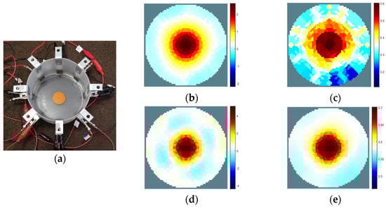
Figure 22.
(a) A carrot slice at the centre of the EIT domain. The corresponding reconstructed images for different inverse solvers of (b) GN (NOSER), (c) BP (Naive), (d) TV (Iteration = 1), and (e) TV (Iterations = 2) at 80 kHz, 1 mA, and 2 Vpp excitation. Overall, GN: NOSER performed well considering λ = 0.17, a better shape and size of the carrot were reconstructed with less noise.

Table 1.
Calculated mean and standard deviation (SD) of obtained changes of conductivity by varying inverse solvers considering a carrot slice in the EIT domain.
Variation of FEM models: The carrot slice (h = 1/5-inch, and D = 25.4 mm) at the centre of the EIT domain was reconstructed onto elements and nodes in the frame by varying FEM models. The results were observable using an ‘a2c0’ (nodes: 41, elements: 64, boundary: 16) or a ‘b2c0’ (nodes: 145, elements: 256, boundary: 32) model and a comparative study was made, as shown in Figure 23. The reconstruction onto elements contributed to obtaining clear images. On the other hand, the reconstructed image onto nodes was found blurred because of the lower number of calculated conductivity data than using elements of the model as shown in Figure 23c,d. The model with a higher vertex density (such as d) represented the finer mesh that can provide a more accurate result in reconstruction than the coarse mesh obtained using a lower vertex density (such as a or b). A good reconstruction of the carrot slice was observed by increasing the vertex density, although the overall conductivity was reduced. The number of conductivity data were increased with the increased elements of the ‘b2c0’ model. Finally, the ‘distmesh’ model using ‘d2d4c’ (nodes: 2507, elements: 4757, boundary: 255) performed well compared to the other FEM models and a good reconstruction was made with more confined results using the optimized GN algorithm: GHPF (λ = 0.17). A good conductivity distribution was found by increasing the number of elements in the frame. The obtained changes of conductivity results are presented in Table 2.

Figure 23.
Reconstructed images of a carrot slice at the centre of an EIT domain for different FEM models at 80 kHz, 1 mA, and 2 Vpp excitation. (a) FEM (a2c0, 8)-elements, (b) corresponding reconstructed slices, (c) FEM (a2c0, 8)-nodes, (d) corresponding reconstructed slices, (e) FEM (b2c0, 8)-elements, (f) FEM (d2d4c, 8)-elements, and (g) corresponding reconstructed slices. A blurred reconstructed image was observed for the reconstruction onto nodes, on the other hand, a good reconstruction was made onto elements. A clear reconstructed image of the carrot slice with an accurate shape was found using a ‘distmesh’ generator FEM model such as ‘d2d4c’ considering the reconstruction onto elements. Overall, the error was decreased by increasing the number of elements.
Table 2.
Calculated mean and standard deviation (SD) of obtained changes of conductivity by varying FEM models considering a carrot slice in the EIT domain.
Variation of number of measurements in the frame: In addition, the number of measurements was reduced from 64 to 40 from the dataset with the target of minimizing the overlapping. In this case, the selected ports (3-4, 3-5, 3-6, 3-7, and 3-8 electrode pairs with respect to electrode 3; 4-5, 4-6, 4-7, 4-8, and 4-1 electrode pairs with respect to electrode 4; and so on) are exactly the same as considered in the four-pole method. Finally, the overlapping was reduced fully considering 28 measurements using the selected ports (1-2, 1-3, 1-4, 1-5, 1-6, 1-7, and 1-8 electrode pairs with respect to electrode 1; 2-3, 2-4, 2-5, 2-6, 2-7, and 2-8 electrode pairs with respect to electrode 2; and so on). The shape, size, and conductivity of the inhomogeneity obtained using the NOSER, Laplace, and Tikhonov algorithms were affected highly for a lower number of boundary voltages data. On the other hand, the distributed conductivity, shape, and size of the sample obtained by the corresponding reconstructed images were not affected highly using GHPF. A comparative study was made between NOSER and GHPF considering a metal inhomogeneity in the EIT domain (shown in Figure 14a), and the obtained results for different measurements at 5 kHz and 1 mA are presented in Figure 24. Overall, GHPF performed well considering the number of measurements of 64/40/28 in the frame compared to the other GN algorithm.
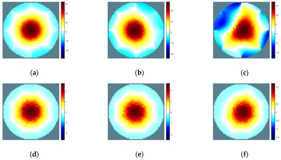
Figure 24.
Reconstructed images of a metal inhomogeneity at the centre of EIT domain by varying the number of measurements of (a) 64, (b) 40, (c) 28 considering NOSER, and (d) 64, (e) 40, (f) 28 considering GHPP with λ = 0.17 at 5 kHz, 1 mA, and 2 Vpp excitation. The maximum conductivity changes was decreased by decreasing the number of measurements and a distorted reconstructed image was found for lower number of measurements using NOSER. The obtained maximum changes of conductivity using GHPF are 2.78, 2.57, and 1.72 S/m, respectively, whereas the changes are very high using NOSER.
The designed EIT sensor system is found suitable to reconstruct and differentiate the conductivity levels of bio-, conductive-, and non-conductive targets with less attenuation. Single or mixed inhomogeneities in the domain and the corresponding positions can be identified successfully considering 2D or 3D EIT and the useful information can be obtained by measuring impedances at different frequencies. A high-speed data acquisition using AD5933 is possible by the in situ measurements precisely up to 100 kHz. A successful evaluation on anomaly detection is made using the designed EIT sensor system as shown in Figure 14, which is very useful in the diagnosis of any abnormalities. The sensor system is found repeatable, and less error is found in multiple measurements for a short duration. The method is found robust and rapid in measurements to analyze the plant traits.
In this work, different samples of multiple plant species were taken for the investigation using 2D and 3D EIT measurements. The samples of different edible plant slices such as two carrots, one radish, and one potato species were taken for 2D operations. In addition, a total of six root samples of different plant species such as four carrot roots (tap roots), one potato root (tap root), and one Pilea root were taken for 3D operations. The root systems of different plants were examined by measuring impedances using the designed EIT sensor system in a controlled environment. The changes in dimensions of a tap root (such as a carrot) were identified and the reconstructions were made successfully by the calculated conductivity from the measured impedances as shown in Figure 16. The biomass was varied with the variation of dimensions of the roots (such as carrot samples) and a good correlation was found with the measured impedances at high frequencies as shown in Figure 17. The root size was found highly correlated with the measured impedances of the root samples.
The root distributions and density of the potato and Pilea roots were identified in different layers of the electrode array as shown in Figure 19 and Figure 20, respectively. The root structures were reconstructed by calculating the conductivity distributed in different layers of the electrode array. The variations in the root systems were able to be detected with the help of 3D imaging. Finally, the biomass of a Pilea root was estimated using EIS measurements with the help of AD5933 and a good correlation with R2 = 0.983 was found considering eight samples in the dataset by the day-wise measurements as shown in Figure 21. A model for root biomass estimation was predicted by selecting features in different frequencies, as shown in Equation (15). It is evident that the tomographic results can be utilized considering multi-electrodes measurements in different layers of the array for monitoring root growth and biomass estimation of the roots in future. The root growth can be monitored in hydroponics or soil media in further experiment. In addition, more useful information of the roots can be obtained by increasing the number of layers of electrodes.
Overall, the output excitation and frequency played an important role in reconstruction analysis. The output of AD5933 was found stable at a 2 Vpp excitation and the samples were found more conductive at the high frequencies. The selection of frequency and the hyperparameter value depended on the type of inhomogeneity in the domain. The conductivity was improved with a lower value of the hyperparameter. The designed electrode array system has a good current carrying capability and is suitable for measuring impedances in a large range of frequencies. The data measured using the sensor system were found suitable for the estimation performance. The developed EIT data acquisition system was tested by the experiments and found suitable for real-time high-precision multifrequency measurements and monitoring in plant phenotyping.
The EIS tools such as the Agilent 4284A LCR meter in addition with Agilent34970A digital multimeter for measuring boundary voltage/current data [1], and the QuadTech 7600 impedance analyzer for measuring bioimpedance [11] utilized in different experiments are very expensive and heavier in weight. On the other hand, a portable, lightweight, and low-cost EIS tool: EVAL-AD5933EBZ, is proposed in this work for developing an automated, reliable, high-precision with good accuracy, and rapid EIT data acquisition system applicable for plant phenotyping. A comparative study was made with the previous research works on the development of the EIT data acquisition system, as shown in Table 3.
Table 3.
A comparison of the features of proposed EIT data acquisition system with the previous research works.
5. Conclusions
In this work, a multifrequency EIT data acquisition system is developed for applications in plant phenotyping with the target of evaluation and 2D/3D reconstruction of the inhomogeneities by measuring impedances in a non-destructive manner. The developed EIT system is portable, low-cost, and radiation-free. The reconstruction performance is evaluated by several algorithms and a comparative study is made. The tomography results of multiple plant roots using the EIT sensor system are obtained successfully in the 3D plane considering the GN: NOSER algorithm. The designed electrode array sensor system is found suitable for in situ measurements and the developed EIT system can be utilized in the field scale for future study.
Author Contributions
R.B. performed the experiments and analyzed the data. R.B. and K.A.W. wrote the draft of the manuscript. K.A.W. suggested for the experiments and data analysis. K.A.W. secured funding for this work. All authors have read and agreed to the published version of the manuscript.
Funding
This work is supported by the Canada First Research Excellence Fund (CFREF) through the Global Institute for Food Security (GIFS), University of Saskatchewan, Canada (422018).
Data Availability Statement
Data is contained within the article.
Acknowledgments
The authors would like to extend their appreciation to the Department of Electrical and Computer Engineering, University of Saskatchewan, for the administrative and technical support for the experiment.
Conflicts of Interest
The authors declare no conflict of interest.
References
- Kim, B.S.; Khambampati, A.K.; Jang, Y.J.; Kim, K.Y.; Kim, S. Image reconstruction using voltage–current system in electrical impedance tomography. Nuclear Eng. Des. 2014, 278, 134–140. [Google Scholar] [CrossRef]
- Bera, T.K.; Nagaraju, J. A MATLAB-Based Boundary Data Simulator for Studying the Resistivity Reconstruction Using Neighbouring Current Pattern. J. Med. Eng. 2013, 2013, 1–15. [Google Scholar] [CrossRef] [PubMed] [Green Version]
- Wang, H.; Liu, K.; Wu, Y.; Wang, S.; Zhang, Z.; Li, F.; Yao, J. Image Reconstruction for Electrical Impedance Tomography Using Radial Basis Function Neural Network Based on Hybrid Particle Swarm Optimization Algorithm. IEEE Sens. J. 2021, 21, 1926–1934. [Google Scholar] [CrossRef]
- Russo, S.; Nefti-Meziani, S.; Carbonaro, N.; Tognetti, A. A Quantitative Evaluation of Drive Pattern Selection for Optimizing EIT-Based Stretchable Sensors. Sensors 2017, 17, 1999. [Google Scholar] [CrossRef] [PubMed]
- Loyola, B.R.; Saponara, V.L.; Loh, K.J.; Briggs, T.M.; O’Bryan, G.; Skinner, J.L. Spatial Sensing Using Electrical Impedance Tomography. IEEE Sens. J. 2013, 13, 2357–2367. [Google Scholar] [CrossRef]
- Yang, Y.; Jia, J.; Smith, S.; Jamil, N.; Gamal, W.; Bagnaninchi, P. A Miniature Electrical Impedance Tomography Sensor and 3D Image Reconstruction for Cell Imaging. IEEE Sens. J. 2017, 17, 514–523. [Google Scholar] [CrossRef] [Green Version]
- Malone, E.; dos Santos, G.S.; Holder, D.; Arridge, S. Multifrequency Electrical Impedance Tomography Using Spectral Constraints. IEEE Trans. Med. Imaging 2014, 33, 340–350. [Google Scholar] [CrossRef]
- Liu, S.; Huang, Y.; Wu, H.; Tan, C.; Jia, J. Efficient Multi-Task Structure-Aware Sparse Bayesian Learning for Frequency-Difference Electrical Impedance Tomography. IEEE Trans. Ind. Inform. 2021, 17, 463–472. [Google Scholar] [CrossRef] [Green Version]
- Malone, E.; dos Santos, G.S.; Holder, D.; Arridge, S. A Reconstruction-Classification Method for Multifrequency Electrical Impedance Tomography. IEEE Trans. Med. Imaging 2015, 34, 1486–1497. [Google Scholar] [CrossRef]
- Singh, G.; Anand, S.; Lall, B.; Srivastava, A.; Singh, V. A Low-Cost Portable Wireless Multi-frequency Electrical Impedance Tomography System. Arab. J. Sci. Eng. 2019, 44, 2305–2320. [Google Scholar] [CrossRef]
- Bera, T.K.; Nagaraju, J.; Lubineau, G. Electrical impedance spectroscopy (EIS)-based evaluation of biological tissue phantoms to study multifrequency electrical impedance tomography (Mf-EIT) systems. J. Vis. 2016, 19, 691–713. [Google Scholar] [CrossRef]
- Shi, X.; Li, W.; You, F.; Huo, X.; Xu, C.; Ji, Z.; Liu, R.; Liu, B.; Li, Y.; Fu, F.; et al. High-Precision Electrical Impedance Tomography Data Acquisition System for Brain Imaging. IEEE Sens. J. 2018, 18, 5974–5984. [Google Scholar] [CrossRef]
- Sapuan, I.; Yasin, M.; Ain, K.; Apsari, R. Anomaly Detection Using Electric Impedance Tomography Based on Real and Imaginary Images. Sensors 2020, 20, 1907. [Google Scholar] [CrossRef] [PubMed] [Green Version]
- Bai, X.; Liu, D.; Wei, J.; Bai, X.; Sun, S.; Tian, W. Simultaneous Imaging of Bio- and Non-Conductive Targets by Combining Frequency and Time Difference Imaging Methods in Electrical Impedance Tomography. Biosensors 2021, 11, 176. [Google Scholar] [CrossRef]
- Weigand, M.; Kemna, A. Multi-frequency electrical impedance tomography as a non-invasive tool to characterize and monitor crop root systems. Biogeosciences 2017, 14, 921–939. [Google Scholar] [CrossRef] [Green Version]
- Weigand, M.; Kemna, A. Imaging and functional characterization of crop root systems using spectroscopic electrical impedance measurements. Plant Soil 2019, 435, 201–224. [Google Scholar] [CrossRef] [Green Version]
- Postic, F.; Doussan, C. Benchmarking electrical methods for rapid estimation of root biomass. Plant Methods 2016, 12, 33. [Google Scholar] [CrossRef] [Green Version]
- Corona-Lopez, D.D.J.; Sommer, S.; Rolfe, S.A.; Podd, F.; Grieve, B.D. Electrical impedance tomography as a tool for phenotyping plant roots. Plant Methods 2019, 15, 49. [Google Scholar] [CrossRef] [Green Version]
- Liu, S.; Jia, J.; Zhang, Y.D.; Yang, Y. Image Reconstruction in Electrical Impedance Tomography Based on Structure-Aware Sparse Bayesian Learning. IEEE Trans. Med. Imaging 2018, 37, 2090–2102. [Google Scholar] [CrossRef] [Green Version]
- Liu, D.; Khambampati, A.K.; Du, J. A Parametric Level Set Method for Electrical Impedance Tomography. IEEE Trans. Med. Imaging 2018, 37, 451–460. [Google Scholar] [CrossRef]
- Yang, Y.; Jia, J. An Image Reconstruction Algorithm for Electrical Impedance Tomography Using Adaptive Group Sparsity Constraint. IEEE Trans. Inst. Meas. 2017, 66, 2295–2305. [Google Scholar] [CrossRef] [Green Version]
- Ren, S.; Wang, Y.; Liang, G.; Dong, F. A Robust Inclusion Boundary Reconstructor for Electrical Impedance Tomography with Geometric Constraints. IEEE Trans. Inst. Meas. 2019, 68, 762–773. [Google Scholar] [CrossRef]
- Zamora-Arellano, F.; López-Bonilla, O.R.; García-Guerrero, E.E.; Olguín-Tiznado, J.E.; Inzunza-González, E.; López-Mancilla, D.; Tlelo-Cuautle, E. Development of a Portable, Reliable and Low-Cost Electrical Impedance Tomography System Using an Embedded System. Electronics 2021, 10, 15. [Google Scholar] [CrossRef]
- Aris, W.; Endarko. Design of low-cost and high-speed portable two-dimensional electrical impedance tomography (EIT). Int. J. Eng. Technol. 2018, 7, 6458–6463. [Google Scholar]
- Ozier-Lafontaine, H.; Bajazet, T. Analysis of root growth by impedance spectroscopy (EIS). Plant Soil 2005, 277, 299–313. [Google Scholar] [CrossRef]
- Liao, A.; Zhou, Q.; Zhang, Y. Application of 3D electrical capacitance tomography in probing anomalous blocks in water. J. Appl. Geophys. 2015, 117, 91–103. [Google Scholar] [CrossRef]
- Newill, P.; Karadaglic, D.; Podd, F.; Grieve, B.D.; York, T.A. Electrical impedance imaging of water distribution in the root zone. Meas. Sci. Technol. 2014, 25, 055110. [Google Scholar] [CrossRef] [Green Version]
- Tan, C.; Liu, S.; Jia, J.; Dong, F. A Wideband Electrical Impedance Tomography System based on Sensitive Bioimpedance Spectrum Bandwidth. IEEE Trans. Inst. Meas. 2020, 69, 144–154. [Google Scholar] [CrossRef]
- Chowdhury, R.I.; Basak, R.; Wahid, K.A.; Nugent, K.; Baulch, H. A Rapid Approach to Measure Extracted Chlorophyll-a from Lettuce Leaves using Electrical Impedance Spectroscopy. Water Air Soil Pollut. 2021, 232, 73. [Google Scholar] [CrossRef]
- Graham, B.M.; Adler, A. Electrode placement configurations for 3D EIT. Physiol. Meas. 2007, 28, 29–44. [Google Scholar] [CrossRef]
- Basak, R.; Wahid, K.; Dinh, A. Determination of Leaf Nitrogen Concentrations Using Electrical Impedance Spectroscopy in Multiple Crops. Remote Sens. 2020, 12, 566. [Google Scholar] [CrossRef] [Green Version]
- Matsiev, L. Improving Performance and Versatility of Systems Based on Single-Frequency DFT Detectors Such as AD5933. Electronics 2015, 4, 1–34. [Google Scholar] [CrossRef] [Green Version]
- Basak, R.; Wahid, K.A.; Dinh, A. Estimation of the Chlorophyll-A Concentration of Algae Species Using Electrical Impedance Spectroscopy. Water 2021, 13, 1223. [Google Scholar] [CrossRef]
- Putensen, C.; Hentze, B.; Muenster, S.; Muders, T. Electrical Impedance Tomography for Cardio-Pulmonary Monitoring. J. Clin. Med. 2019, 8, 1176. [Google Scholar] [CrossRef] [Green Version]
- Rymarczyk, T.; Kłosowski, G.; Kozłowski, E.; Tchórzewski, P. Comparison of Selected Machine Learning Algorithms for Industrial Electrical Tomography. Sensors 2019, 19, 1521. [Google Scholar] [CrossRef] [Green Version]
- Fernández-Fuentes, X.; Mera, D.; Gómez, A.; Vidal-Franco, I. Towards a Fast and Accurate EIT Inverse Problem Solver: A Machine Learning Approach. Electronics 2018, 7, 422. [Google Scholar] [CrossRef] [Green Version]
- Kłosowski, G.; Rymarczyk, T.; Niderla, K.; Rzemieniak, M.; Dmowski, A.; Maj, M. Comparison of Machine Learning Methods for Image Reconstruction Using the LSTM Classifier in Industrial Electrical Tomography. Energies 2021, 14, 7269. [Google Scholar] [CrossRef]
Publisher’s Note: MDPI stays neutral with regard to jurisdictional claims in published maps and institutional affiliations. |
© 2022 by the authors. Licensee MDPI, Basel, Switzerland. This article is an open access article distributed under the terms and conditions of the Creative Commons Attribution (CC BY) license (https://creativecommons.org/licenses/by/4.0/).