Abstract
Airborne array tomographic synthetic aperture radar (TomoSAR) is a major breakthrough, which can obtain three-dimensional (3D) information of layover scenes in a single pass. As a high-resolution SAR, airborne array TomoSAR has considerable potential for 3D applications. However, the original TomoSAR elevation resolution is limited by the baseline and platform length. In this study, a novel method for enhancing the elevation resolution is proposed. First, the actual curve trajectory observation model of airborne array TomoSAR is established. Subsequently, multi-channel image data are substituted into the model to obtain the observation equation. Furthermore, the azimuth and elevation directions of the two-dimensional observation scene are modeled uniformly. The scene reconstruction is realized through the two-dimensional joint solution. Finally, the observation equation is sparsely solved according to the sparse distribution characteristics of the target to obtain the image. The performance of the proposed method is verified via simulation and real-data experiments. The experimental results indicate that, compared with the traditional elevation resolution enhancement method, the proposed method improves the elevation resolution by two times. The proposed method also provides a new thinking for high-resolution SAR 3D imaging.
1. Introduction
Airborne array tomographic synthetic aperture radar (TomoSAR) imaging technology is a major breakthrough, which can obtain the elevation information of layover scenes, such as high mountains and layover buildings [1]. Owing to its advantage that three-dimensional (3D) information can be obtained by a single pass, it shows great application prospects in the 3D application field. In addition, it plays an important role in SAR imaging applications, such as in the field of military reconnaissance [2], topographic surveying [3], resource exploration [4], environmental monitoring [5], crop detection [6,7], and other applications [8,9,10,11].
TomoSAR development history can be traced back to 1995, when K.K.Nell demonstrated that 3D reconstruction can be achieved through TomoSAR. Since then, TomoSAR has been studied in various countries [12]. Deutsches Zentrum für Luft-und Raumfahrt designed the sector imaging radar for enhanced vision [13,14]. Later, Forschungsgesellschaft für Angewandte Naturwissenschaften e.V. designed the airborne radar for three-dimensional imaging and nadir observation (ARTINO) [15]. For the spaceborne TomoSAR system, studies on 3D imaging are classified into two aspects: high-resolution imaging algorithms and applications. The former mainly includes research on motion compensation (MOCO) and enhancement of resolution algorithms. The traditional improved two-step motion compensation (TS-MOCO) algorithm dominates [16]. For elevation resolution enhancement, the compressed sensing (CS) algorithm and its evolution prevail [17,18]. The CS method requires the target distribution to be sparse in the elevation direction, which is mainly divided into two categories. The first is greedy pursuit algorithm, such as the orthogonal matching pursuit algorithm proposed by Sujit Kumar Sahoo et al. [19]. In comparison, the second kind of convex relaxation algorithm, such as the basis pursuit algorithm (BP), proposed by SS Chen et al. [20]. Zhu et al. first proposed a base-tracking minimum parametric method to solve the CS limitation; subsequently, a series of studies based on CS imaging algorithms were conducted [21]. Jiang et al. proposed a new 3D imaging method and used RadarSat-1 data for validation [22]. In the same year, Xu et al. proposed high-resolution imaging based on Bayesian compression perception for imaging scenes with clutter [23]. As for the studies focusing on the application of 3D imaging methods, mainstream methods apply different algorithms to different situations, such as forests and buildings [24]. Many scholars have conducted extensive research on 3D imaging with fruitful results in sparse imaging algorithms and other aspects [25,26].
Although widespread research on TomoSAR 3D imaging has achieved promising results, existing studies have certain limitations. First, flight-pass distribution is nonuniform, which causes high side lobes in TomoSAR imaging, thereby making some ideal algorithms inapplicable [27]. Second, the flight-pass number is insufficient. To avoid spatial fuzzy, sampling needs to satisfy Nyquist theorem, which requires a sufficiently small flight-pass interval and sufficient flight-pass data to ensure high-resolution imaging. However, obtaining sufficient flight-pass data are not only costly but also impractical [28]. Airborne array TomoSAR can solve the abovementioned problems by placing several antennas along the cross-track direction to provide data supporting 3D imaging [8]. In 2014, the National Key Laboratory of Microwave Imaging Technology and the Institute of Electronics, Chinese Academy of Sciences, developed the first airborne array TomoSAR system in China [29]. Since 2015, based on this system, numerous experiments have been conducted for buildings and mountainous areas [30]. Moreover, a series of high-precision imaging algorithms have been presented. In 2017 and 2018, Li et al. presented a Gaussian mixture model 3D imaging method based on CS [31] and group sparsity 3D reconstruction method [32]. In 2018, Li et al. proposed an automatic focus algorithm based on topography search [33]. In the same year, Wang et al. proposed an algorithm based on spatial clustering seed growth for point cloud filtering [34], while Cheng et al. demonstrated multiple scattering of typical structures in urban areas [35,36]. In 2020, Jiao et al. demonstrated 3D imaging using a contextual information approach with a statistical method [37].
In summary, based on airborne array TomoSAR, domestic and foreign scholars have achieved abundant research results [38]. However, the basis of these studies is to compensate for the motion error. In fact, owing to airflow bumps and other factors, aircraft motion is subject to errors, which will change the movement of the aircraft baseline and subsequently extend its physical length in space. However, the relevant studies mainly focus on compensating motion errors [39,40]. This limitation of the baseline length is the reason for the lack of direct application of 3D imaging to enhance the elevation resolution using the motion error.
The existing system’s elevation resolution can be enhanced by the CS algorithm. However, the baseline length of airborne array TomoSAR is limited, which restricts the elevation resolution. To overcome the limitation, this paper proposes elevation resolution enhancement using a non-ideal linear motion error method. The main idea of the proposed method is to exploit the baseline variation due to the motion error. Because of the platform limitation, airborne array TomoSAR has a short baseline length in the cross-track direction. Therefore, it is feasible to use the motion error to enhance the elevation resolution under the limitation. Unlike the conventional imaging approximation methods that lose effective baseline length, the proposed method can break through traditional effective baseline length. The airborne array TomoSAR system can obtain the scene range, azimuth, and elevation 3D spatial spectrum, and the motion error can significantly increase the support domain of the elevation spatial spectrum. Therefore, the proposed method can improve the system’s ability to resolve the elevation direction. The main contributions of the method are as follows: the non-ideal linear motion error is used to enhance the elevation resolution; the baseline length, which is lost in the traditional motion compensation process, is used to the maximum, thus providing a solid foundation for the elevation resolution improvement; and finally, the elevation resolution is enhanced with the loss of azimuth and range resolution, thereby realizing high-resolution 3D imaging.
This paper is organized as follows. In Section 2, the basic principles of the proposed method are introduced in detail. In Section 3, the proposed method for enhancing the elevation resolution is proposed. Section 4 briefly introduces the database of our system. Section 5 presents simulation experiment and real data experiment results. Discussions are given in Section 6. Section 7 presents the conclusions of the paper.
2. Airborne Array TomoSAR Imaging Theory
In this section, the airborne array TomoSAR signal model is first described; then, its spatial spectrum is illustrated. Finally, the use of the motion error to enlarge the effective baseline is demonstrated.
2.1. Airborne Array TomoSAR Signal Model
Airborne array TomoSAR obtains elevation resolution by sequentially adding multiple channels along the cross-range direction, thereby forming a synthetic aperture in the elevation direction. A geometric model of airborne array TomoSAR imaging under an ideal trajectory is shown in Figure 1. In the geodetic coordinate system (x, y, z), axes x, y, and z represent the azimuth, ground, and height directions, respectively. In the radar coordinate system (a, r, s), axes a, r, and s represent the azimuth, range, and elevation directions, respectively. In both radar and geodetic coordinate systems, the three directions are orthogonal to each other. Let us assume that the platform has a uniform linear motion along the azimuth direction. The system works in the side-view mode, and is the central incidence angle.
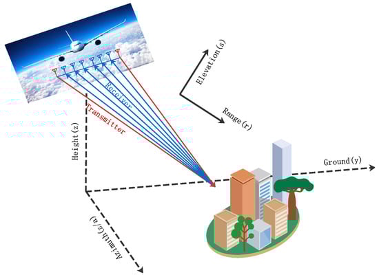
Figure 1.
Geometric model of airborne array TomoSAR imaging under ideal trajectory.
For the point target in the scene, the echoes of the received channel according to the geometric relationship in Figure 1 can be expressed as follows:
where t, , and denote the fast time, the transmit pulse width, and the center frequency, respectively. represents the linear tuning frequency.
For the above imaging geometry model, the airborne array TomoSAR signals are emitted by the array element and received by array elements. The received signal can be expressed as
where denotes the echo of the target sampled at the pulse time and received by the array element at the fast time moment t, and represents the backscattering coefficient of the target . is the echo time delay transmitted from the array element , passing through the point target P in the middle and finally received by the array element ; it is expressed as follows:
where c and denote the speed of light and the spatial distance between the transmitting array element and the observation scene target . is the distance between the observation scene target and the receiving array element .
The signal from Equation (1) after the phase compensation of the original echo can be expressed as follows:
where the azimuth sampling position is a and the cross-course sampling position is l. The compensated echo signal is transformed into the wave-number domain by 3D Fourier transform. It can be shown as follows:
where is the echo signal after compensation by 3D Fourier transform and can be expressed as
where , , and represent the number of range waves, azimuth waves, and cross-course waves, respectively.
is the signal spectrum of the transmitted signal in the wave number domain, and it is expressed as follows:
is the observation target used as the reference point to construct the matched filter, and it is expressed as follows:
Among them:
and
The 3D wave number is subjected to a 3D STOLT transformation, where the mapping relationships are expressed as:
Finally, the 3D distribution of the backscattering coefficients of the observed scene is obtained by performing the 3D Fourier inversion on the results, thus realizing 3D resolution [21].
The echo spectrum of the airborne array TomoSAR signal model contains the 3D spatial spectrum information of the scene. The azimuth spatial spectrum support domain is the azimuth signal bandwidth, and the azimuth antenna length is D, which is expressed as follows:
The spatial spectrum support domain in the range direction is represented as follows:
where and are the carrier frequency and the bandwidth of the transmitting linear frequency modulation (LFM) signal. The spatial spectrum support domain in the elevation direction is as follows:
B, R, and are, respectively, the length of the array antenna, the distance from the scene center, and the viewing angle under the wave number center, respectively. is the distance from the scene target to the antenna, and represents the position where the target deviates from the wave number center [8].
2.2. Effective Baseline Length
Figure 2 shows the geometric relationship of the measured effective baseline length of airborne array TomoSAR under this system. Distances from point on the ground to antennas and are and , respectively. The baseline inclination angle is . B represents the baseline length, which is the distance between two antenna phase centers.
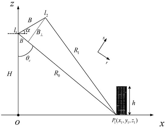
Figure 2.
Geometric relationship of the airborne array TomoSAR measurement baseline length.
The baseline is decomposed along the range direction and the elevation direction perpendicular to the range direction, obtaining parallel and perpendicular baselines, respectively, [24]. In addition, the perpendicular baseline becomes the effective baseline of the airborne array TomoSAR system.
During the actual flight, problems such as air turbulence are encountered, which cause carrier deviation from the original track, producing a motion error. The geometric model of airborne array TomoSAR imaging under the non-ideal track is shown in Figure 3. In the scene, , , and H are the azimuth position of the radar at the moment of mth pulse, the position of the nth array element, and the platform height, respectively.
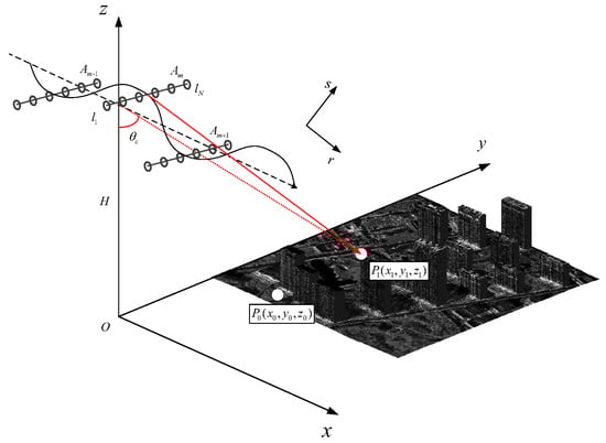
Figure 3.
Geometric model of airborne array TomoSAR imaging under non-ideal trajectory.
Single-point imaging requires an effective irradiation range within the synthetic aperture time. The actual effective baseline length variation projected into the azimuth–elevation geometric plane as shown in Figure 4. The figure clearly shows the antenna array element position with a bump on the platform.
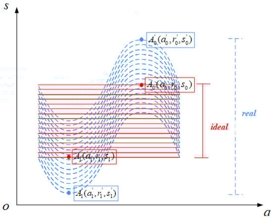
Figure 4.
Trajectory projected into the azimuth–elevation geometric plane.
The blue solid line and red dashed line correspond to the non-ideal track and ideal track. When the baseline length changes from the projection of along the elevation direction to the projection of , the effective baseline length under the non-ideal track and ideal track equations are expressed as follows.
The analysis clearly indicates that the actual effective baseline length is much longer than the fitted effective baseline length. This serves as a solid foundation for the proposed method. With the proposed method that uses the motion error to increase the physical effective baseline, the elevation spatial spectrum can be widened without losing the azimuth and range direction spatial spectra, resulting in the improvement of the elevation resolution.
3. Resolution Enhancement Using the Motion Error Method
This paper presents a method to enhance the original physical effective baseline length by using the motion error of the non-ideal trajectory. This approach is different from the traditional imaging method that compensates the motion error under the non-ideal trajectory. The original physical baseline length is increased by using the non-ideal track motion error. At the same time, the 2D joint modeling of azimuth and elevation is carried out for the observation scene; then, the scene reconstruction is realized by 2D joint solution. The specific implementation steps are as follows:
- 1.
- Airborne array TomoSAR transmits LFM signals to the observation scene and received echo.
- 2.
- Echo data images of each channel are obtained in 2D. Based on the position and orientation system (POS) data, the ranges of non-ideal and ideal trajectories are determined.
- 3.
- Each channel complex image is aligned and the amplitude phase is corrected.
- 4.
- According to the trajectory information and scene grid position, the observation equation is generated.
- 5.
- The conversion result data of ten continuous azimuth pixels along the same distance, which can describe the change in the trajectory in a synthetic aperture, are intercepted in sequence and substituted into the observation equation. The observation equation is solved under the constraint of target sparsity, obtaining the reconstruction results.
- 6.
- The reconstruction results are fused to obtain the 3D reconstruction results of the whole scene.
The proposed airborne array TomoSAR 3D imaging method is shown in Figure 5.
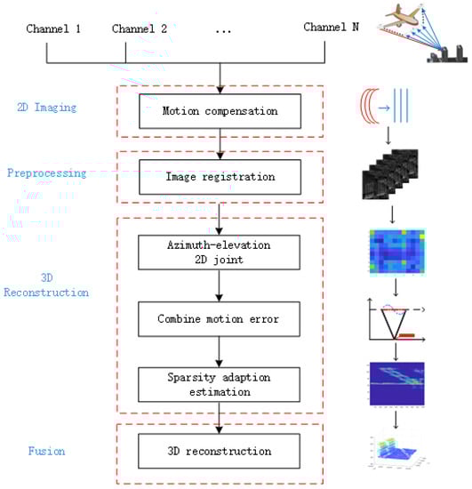
Figure 5.
Improved 3D imaging method.
The specific algorithm of 3D reconstruction is shown in the below Algorithm 1. Following the above processing, 3D reconstruction of the whole scene can be realized.
According to the above steps, the motion error is used to enhance the physical effective baseline length while obtaining a higher elevation resolution in the same case.
| Algorithm 1: 3D Reconstruction. |
Input: Multi-channel image registration data , POS data Initialization: Multi-channel image registration data size for all do Step 1: Ten points in ten azimuth directions are selected one after the other. The azimuth coordinate a and elevation coordinate s are recorded. Step 2: The grid points are divided into . The observation matrix is calculated as , the actual curve trajectory observation model of airborne array TomoSAR is established. for all do Step 3: Starting from one distance direction in sequence, azimuth FFT is performed. The multi-channel image data are substituted into the model to obtain the observation equation. end Step 4: The observation equation is sparsely solved according to the sparse distribution characteristics of the target to obtain the target image. Alternative adaptive estimation in the azimuth frequency domain and elevation time domain. end Output: The 3D reconstruction data . |
4. Datasets
For the simulation and real-data experiments, the result obtained by our team in 2021 using airborne array TomoSAR in Weinan, Shaanxi Province, were used. The system is shown in Figure 6. The system operates in a 2-transmission, 8-receiver mode, and has 16 phase centers in the cross-range direction with 0.2 m spacing between adjacent centers. Other system parameters are shown in Table 1.
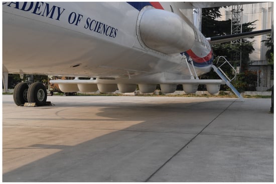
Figure 6.
Airborne array TomoSAR system.

Table 1.
Airborne array TomoSAR parameters.
Based on the parameters, the elevation resolution and ambiguous elevation of the airborne array TomoSAR system can be obtained as follows.
When the separation of two scattering points within a resolution cell is less than 34 m, only a super-resolution method can be used for distinguishing them. Furthermore, the maximum ambiguous elevation of the scene is 534 m. When the beam width is certain, the lower platform height and the smaller shooting angle will have a negative impact of the imaging area. Therefore, the shooting angle of our system is 34, and the flight height of the platform is 4.7 km. The proposed method discusses how to improve the elevation resolution in a given system.
To verify the practicality of the proposed method, we evaluated multiple sets of strip data. One synthetic aperture length was calculated according to the airborne array TomoSAR system parameters, as per the following formula.
where , , and are the subaperture length, closest scene slant distance, and transmit signal beam width, respectively. The total flight length is calculated from , where and are coordinate values corresponding to the start and end of the azimuth direction. The number of subapertures is calculated using . The difference between the highest and lowest points of the projection in POS data, which are along the y and z directions in the elevation upward, is found for each subaperture.
According to the above statistics, there are a total of 2087 strips that meet the requirements. The remaining strip data are the cases of large motion errors caused by non-ideal trajectories comprising bumps. The statistics of motion errors in the synthetic aperture are shown in Figure 7. The vertical coordinate is the number of compliant subapertures and the horizontal coordinate is the specific value of the motion error. Clearly, relatively large motion errors exist in the data. The above analysis proves that the actual data support the proposed method.
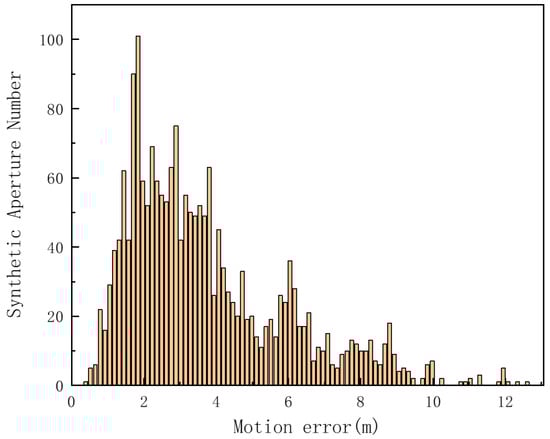
Figure 7.
Subaperture motion error statistics.
5. Experimental Results and Analysis
To verify the effectiveness of the proposed method, first, several simulation experiments are analyzed to compare the reconstruction of the same observation scene. Furthermore, a flight experiment using the airborne array TomoSAR for the urban area of Weinan, Shaanxi Province, are selected; it comprises 3D reconstruction of four sets of layover points and layover buildings. Specifically, due to the BP algorithm has high computational complexity, we compare the convex relaxation algorithm BP in compressed sensing to the proposed method [20].
5.1. Simulation Experiments
Simulation parameters are X-band airborne array TomoSAR parameters, corresponding to the scaling charts of the ideal linear and non-ideal linear trajectories, as shown in Figure 8. The input variable of this simulation is a vector containing complex values, where 10 and 16 are azimuth-direction sampling points and number of elevation direction channels, respectively. The signal-to-noise ratio (SNR) is 30 dB. Other parameters are the same as shown in Table 1. We sampled 400 points uniformly at a 1 m interval along the elevation direction. Two scattering points having the same amplitude and quadrature phase are considered in the simulation.
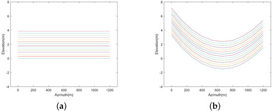
Figure 8.
X-band trajectory. (a) Ideal linear trajectory. (b) Non-ideal linear trajectory.
Figure 8 indicates that the baseline lengths of the ideal and non-ideal linear trajectories are approximately 4 m and 8 m, respectively. From Equation (21) and Table 1, the effective baselines are approximately 3.3 m and 6.6 m. In theory, using the motion error, Rayleigh resolution can reach approximately twice as much as without using the motion error. In other words, under the proposed system, the original Rayleigh resolution form is 34 m, and when the motion error is used, the Rayleigh resolution can reach 17 m.
To illustrate that the proposed method can enhance elevation resolution, we compare the strength of resolution of two scattering points at different intervals. Green, red, and blue represent the results of using the motion error, without using the motion error, and the original reconstruction, respectively. The elevation position of the first scattering point is fixed at 1 m, while the second scattering point gradually approaches the first scattering point in the elevation upward. Elevation intervals of two scattering points are 5 m, 4 m, 3 m, 2 m, and 1 m. The results are shown in Figure 9.
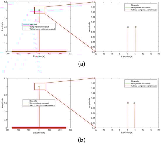
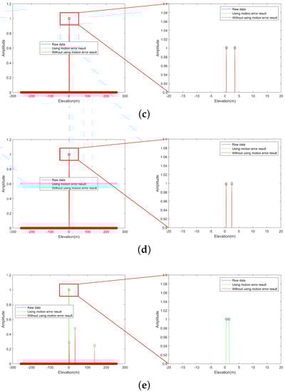
Figure 9.
Comparison of scattering point reconstruction performance (using motion error(the proposed method) compare without using motion error (BP algorithm)). (a) Two targets interval 5 m and zoom of the highest point. (b) Two targets interval 4 m and zoom of the highest point. (c) Two targets interval 3 m and zoom of the highest point. (d) Two targets interval 2 m and zoom of the highest point. (e) Two targets interval 1 m and zoom of the highest point.
Figure 9a–d show effective results of distinguishing two targets by using and without using the motion error when the elevation intervals are 2–5 m. Nevertheless, the discrimination ability of spurious targets and outliers is improved by using the motion error. As Figure 9e shows, when the elevation interval is 1 m, the proposed method using the motion error can effectively distinguish two targets, while the method without using the motion error cannot completely distinguish the targets. Therefore, the proposed method shows great application potential in elevation resolution. The simulation results indicate that the conventional method without using the motion error can achieve a Rayleigh resolution 16 times higher than the theoretical Rayleigh resolution, while the proposed method can achieve 32 times the theoretical Rayleigh resolution.
To evaluate relevant performance, we conducted 100 runs of Monte Carlo experiments with different motion errors, and the results are shown in Figure 10. The ideal linear motion range was fixed while gradually increasing the motion error. Fifteen groups of signals were used for the experiment. The set of effective baseline size ratios of the method using the motion error to the method without using the motion error was shown in Table 2. It can be seen that reconstruction success rate increases significantly with increasing ratio. When the ratio is times, there is already a high probability that the method using the motion error can distinguish targets with 1 m elevation interval. In conclusion, the proposed method can improve the elevation resolution substantially in practical situations.
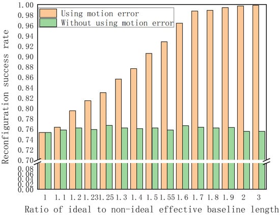
Figure 10.
Performance evaluation of the proposed method.
Table 2.
Effective baseline size ratios.
5.2. Real-Data Experiments
5.2.1. Layover Points
Target area reconstruction scene is a calibration field with multiple sets of layover points. The SAR image is shown in Figure 11, wherein the highlighted strong scattering points are the calibration points. Four strong scattering points are located on a flat field. Figure 12 shows the physical drawing of layover scalers.
Figure 11.
Layover points 2D SAR imaging.
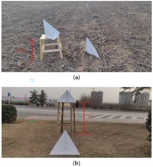
Figure 12.
Layover scalers physical drawing. (a) Two targets interval 0.5 m. (b) Two targets interval 1 m.
Four sets of layover points are selected with elevation intervals of 1 m and 0.5 m. The 2D imaging plots of the four sets of layover points are shown in Figure 13. In Figure 13a, at the 96th grid in the azimuth direction is the 1st set of layover points, while at the 110th grid in the azimuth direction is the 2nd set of layover points. In Figure 13b, at the 98th grid in the azimuth direction is the 3rd set of layover points, while at the 104th grid in the azimuth direction is the 4th set of layover points.
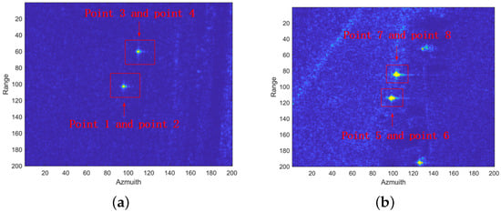
Figure 13.
Four groups layover points. (a) On the 96th and 110th grids are the 0.5 m and 1 m layover points. (b) On the 98th and 104th grids are 1 m and 1 m layover points.
The four sets of layover points are reconstructed using the motion error and the traditional BP algorithm. The reconstruction results of the four sets of layover points are given in Figure 14.
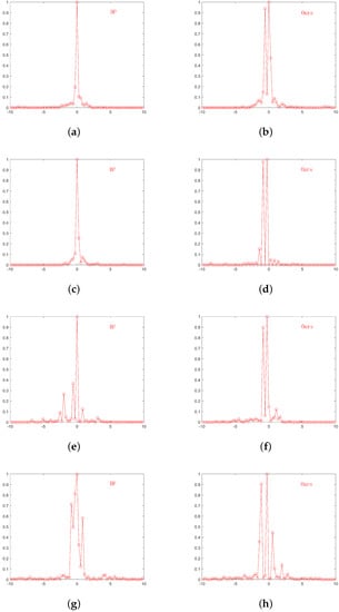
Figure 14.
Comparison of reconstruction performance in layover points. (a) BP reconstruction result of point 1 and point 2. (b) Proposed method reconstruction result of point 1 and point 2. (c) BP reconstruction result of point 3 and point 4. (d) Proposed method reconstruction result of point 3 and point 4. (e) BP reconstruction result of point 5 and point 6. (f) Proposed method reconstruction result of point 5 and point 6. (g) BP reconstruction result of point 7 and point 8. (h) Proposed method reconstruction result of point 7 and point 8.
The total number of reconstruction grid points for the first set of layover points is 2134, with a spacing of 0.25 m between adjacent grid points. Figure 14a,b show the results of the orientation cumulative reconstruction using the BP algorithm and the proposed method for points 1 and 2, with an elevation interval of 0.5 m. Clearly, the reconstruction using the BP algorithm cannot successfully distinguish the two scattering points, whereas the proposed method can identify the two scattering points. In general, the method using the motion error can distinguish two layover points with an elevation interval of 0.5 m. The number of total reconstruction grid points for the remaining sets of layover points is 1068, with a spacing of 0.5 m between adjacent grid points. Figure 14c,d show the results of the orientation cumulative reconstruction using the BP algorithm and the method using the motion error for points 3 and 4, with an elevation interval of 1 m. Clearly, the BP algorithm still cannot distinguish the two scattering points, whereas the proposed method can. Figure 14e,f show the results of the orientation cumulative reconstruction using the BP algorithm and the proposed method for points 5 and 6, with an elevation interval of 1 m. The results indicate that the proposed method can effectively distinguish the two scattering points and shows higher robustness compared with the BP algorithm. Figure 14g,h show the results of the orientation cumulative reconstruction using the BP algorithm and the proposed method using the motion error for points 7 and 8, with an elevation interval of 1 m. Clearly, the reconstruction results of the BP algorithm show many points, while the proposed method have only two strong points even at an elevation interval of 1.5 m. The proposed method can distinguish four layover points with an elevation interval of 1 m and shows better performance than BP algorithm. Furthermore, the reconstruction amplitude of the proposed method was evaluated.
The reconstruction time of the two methods was measured, and the comparison of statistical results is shown in Table 3.
Table 3.
Reconstruction time.
The reconstruction results of the four sets of layover points show that irrespective of the distance between layover points (i.e., 1 m or 0.5 m), the proposed method can successfully distinguish the points.
5.2.2. Layover Building
Furthermore, reconstruction of an urban building was processed, whose 2D SAR imaging is shown in Figure 15.
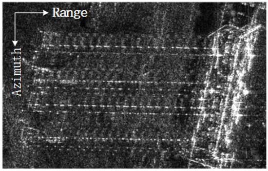
Figure 15.
Processing building 2D SAR imaging.
The azimuth cumulative reconstruction results of the building obtained using the proposed method are shown in Figure 16.
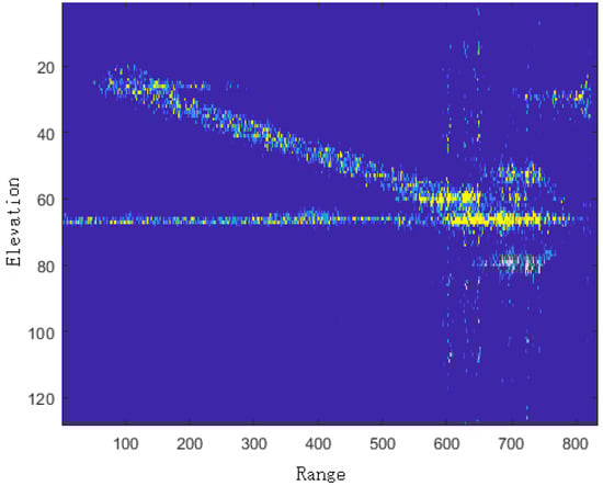
Figure 16.
Azimuth cumulative display of building reconstruction results.
The 3D reconstruction result is shown in Figure 17.
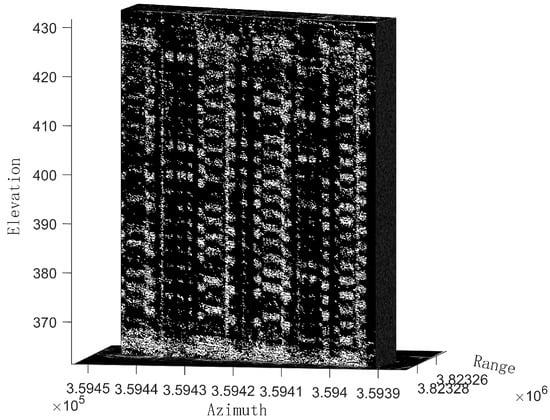
Figure 17.
3D reconstruction result.
The above simulation and actual overlay reconstruction results show that the proposed method can achieve about 34 times the resolution of the Rayleigh resolution and 2 times the resolution of the BP algorithm. It can distinguish overlay points with elevation spacing of 0.5 m and 1 m. At the same time, it is illustrated by the reconstruction results of a single building.
6. Discussion
Simulation and airborne array TomoSAR system results show the effectiveness of the proposed method to improve elevation resolution by using motion error. The simulation results show that the proposed method improves the elevation Rayleigh resolution by using motion error. It can be seen from the simulation results that with the increase in the effective baseline length, the resolution success rate also increases. At the same time, the elevation resolution is more than twice that of BP algorithm, reaching 1 m, and the error is about 0.05 m (e.g., Figure 9), which reflects higher accuracy and robustness. The algorithm is applied to airborne array TomoSAR system to verify the effectiveness of this method in improving elevation resolution. The layover points of 0.5 m and 1 m elevation can be distinguished. At the same time, a layover building is reconstructed by this method. In the simulation, although the Rayleigh resolution of the system is only 34 m, the proposed method can distinguish the super-resolution of two targets with an elevation interval of 1 m (e.g., Figure 14). The resolution results in the elevation direction of airborne array TomoSAR show the same super-resolution performance, except that the fourth group of points are located at the far end of the scene with a little error (e.g., Figure 14h). At the same time, to our surprise, the elevation spacing of 0.5 m can also be resolved (e.g., Figure 14a).
As mentioned earlier, our proposed algorithm can increases the effective baseline length, which therefore improves the elevation resolution. It is important because baseline length and elevation resolution are key parameters in 3D imaging. The algorithm can obtain higher super-resolution performance in the elevation direction. Although the proposed algorithm has high accuracy, there are other tasks to be completed: first, the proposed method is at the cost of more time. The subsequent research needs to balance time cost and computing efficiency. In addition, the proposed method needs to use the motion error in the aperture many times, so it is suitable for the system of wide-beam transmission. The elevation resolution improvement of narrow-beam systems needs further research.
7. Conclusions
High-resolution 3D reconstruction technology is of great significance in urban surveying, environmental monitoring, and other fields. However, the elevation resolution obtained by existing methods is inconsistent owing to the inherent characteristics of the baseline length. In addition, the existing motion error analysis technology focuses on compensating the motion error. This paper described these problems in detail and proposed a method to improve the elevation resolution by using the motion error to enhance the baseline length. In addition, the spectrum correspondence rule was analyzed. First, the actual curve trajectory observation model of airborne array TomoSAR was established. Subsequently, multi-channel image data were substituted into the model to obtain the observation equation. Finally, the observation equation was sparsely solved according to the sparse distribution characteristics of the target to obtain the target image. The simulation and real-data experiments showed that when the ratio of the actual and fitting effective baseline length is two, while the resolution should also be twice the quality. The reconstruction results obtained using the BP algorithm and the proposed method were compared. The proposed method can accurately identify overlay points with elevation interval of 1 m or higher. It could also distinguish the points at an elevation interval of 0.5 m, although the side lobe was high. The results confirmed that the proposed method has broad application prospects in high-resolution SAR 3D imaging.
In a future study, we will focus on balancing higher resolution and the execution time.
Author Contributions
Conceptualization, L.Y., F.Z., and Z.Z.; data curation, F.Z. and D.W.; formal analysis, Z.Z. and L.C.; funding acquisition, F.Z. and Z.Z.; methodology, L.Y.; project administration, F.Z. and Z.Z.; resources, L.C. and Z.Z.; validation, L.Y., F.Z., Z.Z., and Z.L.; software, L.Y., F.Z., and Y.Y.; writing—original draft preparation, L.Y.; writing—review and editing, L.Y., Z.L., and D.W. All authors have read and agreed to the published version of the manuscript.
Funding
This work was supported by National Key R&D Program of China, 2021YFA0715404.
Data Availability Statement
Not applicable.
Acknowledgments
The authors thank all colleagues who participated in the array TomoSAR system design and the acquisition of measured data. The authors would like to express their gratitude to the anonymous reviewers and the editor for their constructive comments on the paper.
Conflicts of Interest
The authors declare no conflict of interest.
Abbreviations
The following abbreviations are used in this manuscript:
| TomoSAR | tomographic synthetic aperture radar |
| 3D | three-dimensional |
| MOCO | motion compensation |
| 2D | two-dimensional |
| TS-MOCO | two-step motion compensation |
| ARTINO | airborne radar for three-dimensional imaging and nadir observation |
| AIRCAS | Aerospace Information Research Institute, Chinese Academy of Sciences |
| CS | compressed sensing |
| LFM | linear frequency modulation |
| POS | position and orientation system |
| FFT | fast Fourier transform |
| SNR | signal-to-noise ratio |
| BP | basis pursuit |
References
- Shi, J.; Zhang, X.; Yang, J.; Wang, Y. Surface-Tracing-Based LASAR 3-D Imaging Method via Multiresolution Approximation. IEEE Trans. Geosci. Remote Sens. 2008, 46, 3719–3730. [Google Scholar]
- Zhu, X.X.; Montazeri, S.; Gisinger, C.; Hanssen, R.F.; Bamler, R. Geodetic SAR Tomography. IEEE Trans. Geosci. Remote Sens. 2016, 54, 18–35. [Google Scholar] [CrossRef]
- Ishimaru, A.; Chan, T.K.; Kuga, Y. An imaging technique using confocal circular synthetic aperture radar. IEEE Trans. Geosci. Remote Sens. 1998, 36, 1524–1530. [Google Scholar] [CrossRef]
- Mahafza, B.R. Two-dimensional SAR imaging using linear arrays with transverse motion. J. Frankl. Inst. 1992, 330, 95–102. [Google Scholar] [CrossRef]
- Wang, Y.; Wang, B.; Hong, W.; Du, L.; Wu, Y. Imaging Geometry Analysis of 3D SAR using Linear Array Antennas. In Proceedings of the IGARSS 2008-2008 IEEE International Geoscience and Remote Sensing Symposium, Boston, MA, USA, 7–11 July 2008; Volume 3, pp. III-1216–III-1219. [Google Scholar]
- Wei, S.J.; Zhang, X.L.; Shi, J. Compressed sensing Linear array SAR 3-D imaging via sparse locations prediction. In Proceedings of the 2014 IEEE Geoscience and Remote Sensing Symposium, Quebec City, QC, Canada, 13–18 July 2014; pp. 1887–1890. [Google Scholar]
- Wei, S. Fast Bayesian Compressed Sensing Algorithm via Relevance Vector Machine for LASAR 3D Imaging. Remote Sens. 2021, 13, 1751. [Google Scholar] [CrossRef]
- Zhang, F.; Liang, X.; Wu, Y.; Lv, X. 3D surface reconstruction of layover areas in continuous terrain for multi-baseline SAR interferometry using a curve model. Int. J. Remote Sens. 2015, 36, 2093–2112. [Google Scholar] [CrossRef]
- Wei, X.; Chong, J.; Zhao, Y.; Li, Y.; Yao, X. Airborne SAR Imaging Algorithm for Ocean Waves Based on Optimum Focus Setting. Remote Sens. 2019, 11, 564. [Google Scholar] [CrossRef]
- Tsaig, Y.; Donoho, D.L. Extensions of compressed sensing. Signal Process. 2006, 86, 549–571. [Google Scholar] [CrossRef]
- Baraniuk, R.; Steeghs, P. Compressive Radar Imaging. In Proceedings of the 2007 IEEE Radar Conference, Waltham, MA, USA, 17–20 April 2007; pp. 128–133. [Google Scholar]
- Budillon, A.; Evangelista, A.; Schirinzi, G. SAR tomography from sparse samples. In Proceedings of the 2009 IEEE International Geoscience and Remote Sensing Symposium, Cape Town, South Africa, 12–17 July 2009; Volume 4, pp. IV-865–IV-868. [Google Scholar]
- Zhu, X.X.; Bamler, R. Tomographic SAR Inversion by L1 Norm Regularization – The Compressive Sensing Approach. IEEE Trans. Geosci. Remote Sens. 2010, 48, 3839–3846. [Google Scholar] [CrossRef]
- Jiang, C.; Zhang, B.; Zhang, Z.; Hong, W.; Wu, Y. Experimental results and analysis of sparse microwave imaging from spaceborne radar raw data. Sci. China Inf. Sci. 2012, 55, 15. [Google Scholar] [CrossRef]
- Xu, J.; Pi, Y.; Cao, Z. Bayesian compressive sensing in synthetic aperture radar imaging. IET Radar Sonar Navig. 2012, 6, 2–8. [Google Scholar] [CrossRef]
- Kanatsoulis, C.I.; Fu, X.; Sidiropoulos, N.D.; Akakaya, M. Tensor Completion from Regular Sub-Nyquist Samples. IEEE Trans. Signal Process. 2019, 68, 1–16. [Google Scholar] [CrossRef]
- Xu, G.; Liu, Y.; Xing, M. Multi-Channel Synthetic Aperture Radar Imaging of Ground Moving Targets Using Compressive Sensing. IEEE Access 2018, 6, 66134–66142. [Google Scholar] [CrossRef]
- Quan, Y.; Zhang, R.; Li, Y.; Xu, R.; Zhu, S.; Xing, M. Microwave Correlation Forward-Looking Super-Resolution Imaging Based on Compressed Sensing. IEEE Trans. Geosci. Remote Sens. 2021, 59, 8326–8337. [Google Scholar] [CrossRef]
- Sahoo, S.K.; Makur, A. Signal Recovery from Random Measurements via Extended Orthogonal Matching Pursuit. IEEE Trans. Signal Process. 2015, 63, 2572–2581. [Google Scholar] [CrossRef]
- Chen, S.S.; Saunders, D. Atomic Decomposition by Basis Pursuit. Siam Rev. 2001, 43, 129–159. [Google Scholar] [CrossRef]
- Hang, L.I.; Liang, X.; Zhang, F.; Ding, C.; Yirong, W.U. A novel 3-D reconstruction approach based on group sparsity of array InSAR. Sci. Sin. Inf. 2018, 48, 1051–1064. [Google Scholar]
- Li, Y.L.; Liang, X.D.; Ding, C.B.; Zhou, L.J.; Wen, H. A motion compensation approach integrated in the omega-K algorithm for airborne SAR. In Proceedings of the IEEE International Conference on Imaging Systems and Techniques, Manchester, UK, 16–17 July 2012. [Google Scholar]
- Liang, X. An Elevation Ambiguity Resolution Method Based on Segmentation and Reorganization of TomoSAR Point Cloud in 3D Mountain Reconstruction. Remote Sens. 2021, 13, 5118. [Google Scholar] [CrossRef]
- Meng, D.; Xue, L.; Hu, D.; Ding, C.; Liu, J. Topography- and aperture-dependent motion compensation for airborne SAR: A back projection approach. In Proceedings of the Geoscience and Remote Sensing Symposium, Quebec City, QC, Canada, 13–18 July 2014. [Google Scholar]
- Yi, B.; Gu, D.; Shao, K.; Ju, B.; Zhang, H.; Qin, X.; Duan, X.; Huang, Z. Precise Relative Orbit Determination for Chinese TH-2 Satellite Formation Using Onboard GPS and BDS2 Observations. Remote Sens. 2021, 13, 4487. [Google Scholar] [CrossRef]
- Zhang, S.; Chen, B.; Gong, H.; Lei, K.; Shi, M.; Zhou, C. Three-Dimensional Surface Displacement of the Eastern Beijing Plain, China, Using Ascending and Descending Sentinel-1A/B Images and Leveling Data. Remote Sens. 2021, 13, 2809. [Google Scholar] [CrossRef]
- Mourad, M.; Tsuji, T.; Ikeda, T.; Ishitsuka, K.; Senna, S.; Ide, K. Mapping Aquifer Storage Properties Using S-Wave Velocity and InSAR-Derived Surface Displacement in the Kumamoto Area, Southwest Japan. Remote Sens. 2021, 13, 4391. [Google Scholar] [CrossRef]
- Zheng, W.; Hu, J.; Liu, J.; Sun, Q.; Li, Z.; Zhu, J.; Wu, L. Mapping Complete Three-Dimensional Ice Velocities by Integrating Multi-Baseline and Multi-Aperture InSAR Measurements: A Case Study of the Grove Mountains Area, East Antarctic. Remote Sens. 2021, 13, 643. [Google Scholar] [CrossRef]
- de Castro Filho, H.C.; de Carvalho Júnior, O.A.; de Carvalho, O.L.F.; de Bem, P.P.; dos Santos de Moura, R.; de Albuquerque, A.O.; Silva, C.R.; Ferreira, P.H.G.; Guimarães, R.F.; Gomes, R.A.T. Rice Crop Detection Using LSTM, Bi-LSTM, and Machine Learning Models from Sentinel-1 Time Series. Remote Sens. 2020, 12, 2655. [Google Scholar] [CrossRef]
- Hoskera, A.K.; Nico, G.; Irshad Ahmed, M.; Whitbread, A. Accuracies of Soil Moisture Estimations Using a Semi-Empirical Model over Bare Soil Agricultural Croplands from Sentinel-1 SAR Data. Remote Sens. 2020, 12, 1664. [Google Scholar] [CrossRef]
- Xu, L.; Chen, Q.; Zhao, J.J.; Liu, X.W.; Xu, Q.; Yang, Y.H. An Integrated Approach for Mapping Three-Dimensional CoSeismic Displacement Fields from Sentinel-1 TOPS Data Based on DInSAR, POT, MAI and BOI Techniques: Application to the 2021 Mw 7.4 Maduo Earthquake. Remote Sens. 2021, 13, 4847. [Google Scholar] [CrossRef]
- Knaell, K.; Cardillo, G. Radar tomography for the generation of three-dimensional images. Radar Sonar Navig. IEE Proc. 1995, 142, 54–60. [Google Scholar] [CrossRef]
- Krieger, G.; Wendler, M.; Mittermayer, J.; Buckreuss, S.; Witte, F. Sector Imaging Radar for Enhanced Vision. In Proceedings of the German Radar Symposium, Bonn, Germany, 3–5 September 2002. [Google Scholar]
- Giret, R.; Jeuland, H.; Enert, P. A study of a 3D-SAR concept for a millimeter wave imaging radar onboard an UAV. In Proceedings of the European Radar Conference, Amsterdam, The Netherlands, 11–15 October 2004. [Google Scholar]
- Klare, J.; Weiss, M.; Peters, O.; Brenner, A.R.; Ender, J. ARTINO: A New High Resolution 3D Imaging Radar System on an Autonomous Airborne Platform. In Proceedings of the IEEE International Symposium on Geoscience and Remote Sensing, Denver, CO, USA, 31 July–4 August 2006. [Google Scholar]
- Lei, D.; Wang, Y.P.; Wen, H.; Wu, Y.R. Analytic modeling and three-dimensional imaging of downward-looking SAR using bistatic uniform linear array antennas. In Proceedings of the Asian and Pacific Conference on Synthetic Aperture Radar, Huangshan, China, 5–9 November 2007. [Google Scholar]
- Yang, C.; Lv, S.; Hou, Z.; Zhang, Q.; Li, T.; Zhao, C. Monitoring of Land Subsidence and Ground Fissure Activity within the Su-Xi-Chang Area Based on Time-Series InSAR. Remote Sens. 2022, 14, 903. [Google Scholar] [CrossRef]
- Wu, W.J.; Zhang, X.L.; Wei, S.J. Spaceborne-airborne bistatic SAR 3-D imaging using linear array antenna. In Proceedings of the 2015 IEEE 5th Asia-Pacific Conference on Synthetic Aperture Radar (APSAR), Singapore, 1–4 September 2015. [Google Scholar]
- Zhou, H.F.; Li, Y.; Su, Y. Three-dimensional Imaging with Multi-aspect SAR Data. Dianzi Yu Xinxi Xuebao/J. Electron. Inf. Technol. 2014, 35, 2467–2474. [Google Scholar] [CrossRef]
- Qi, W.; Xing, M.; Lu, G.; Zheng, B. High-Resolution Three-Dimensional Radar Imaging for Rapidly Spinning Targets. IEEE Trans. Geosci. Remote Sens. 2008, 46, 22–30. [Google Scholar]


Publisher’s Note: MDPI stays neutral with regard to jurisdictional claims in published maps and institutional affiliations. |
© 2022 by the authors. Licensee MDPI, Basel, Switzerland. This article is an open access article distributed under the terms and conditions of the Creative Commons Attribution (CC BY) license (https://creativecommons.org/licenses/by/4.0/).