
Small Water Body Detection and Water Quality Variations with Changing Human Activity Intensity in Wuhan


Abstract
:
1. Introduction
2. Data
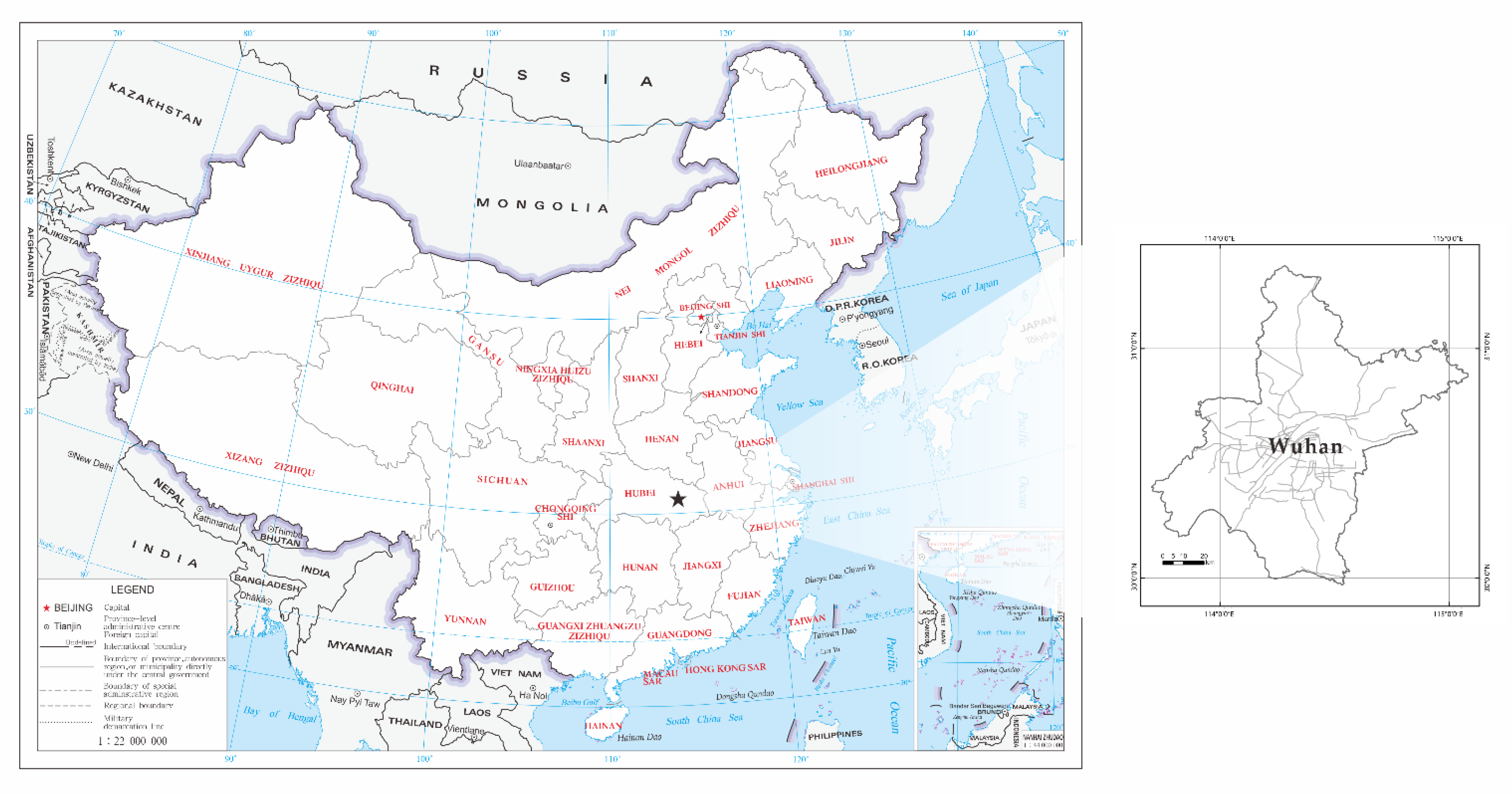
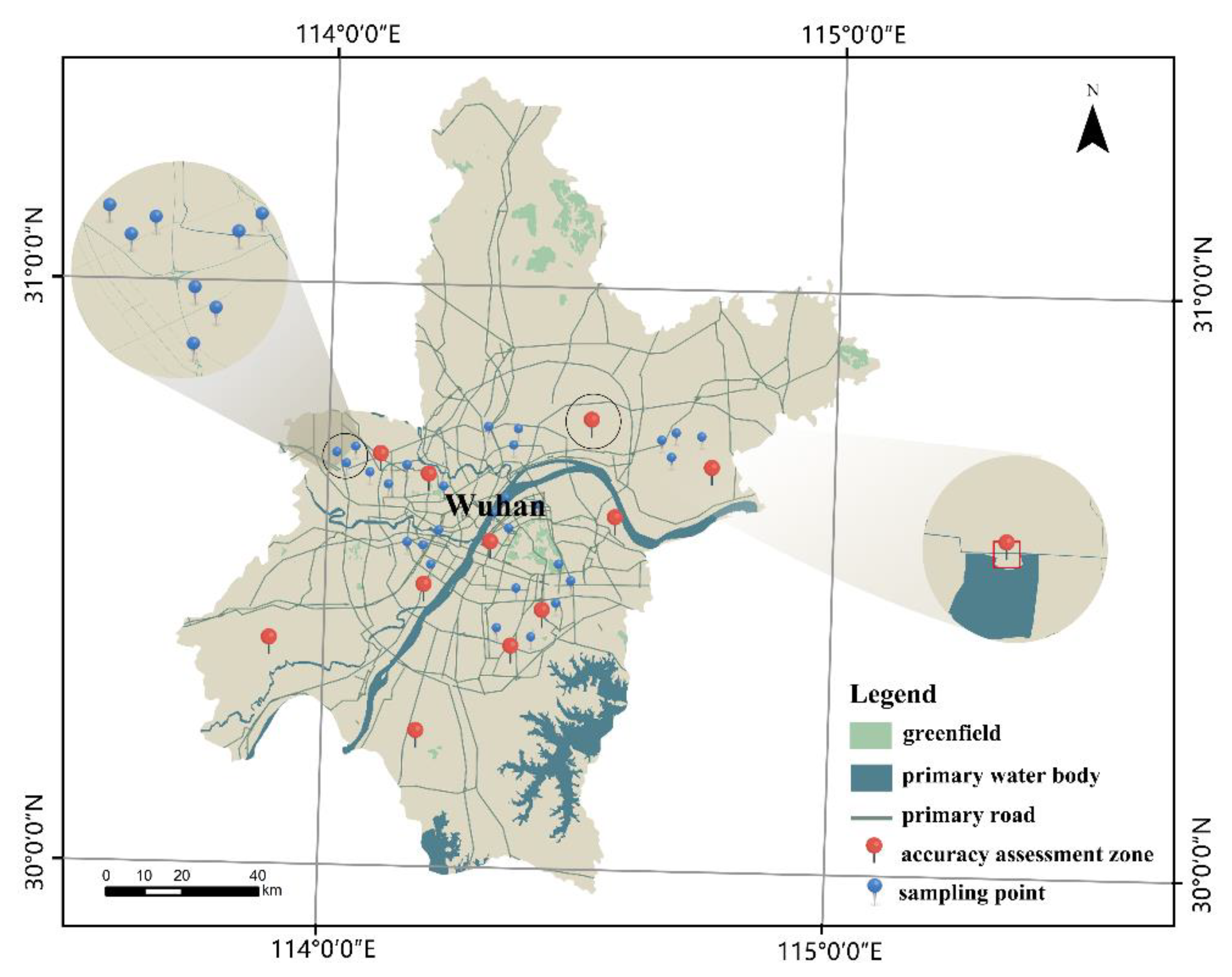
2.1. Study Area
2.2. Remote Sensing Data
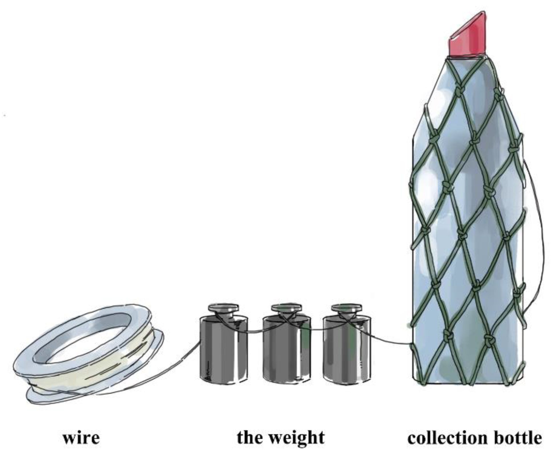
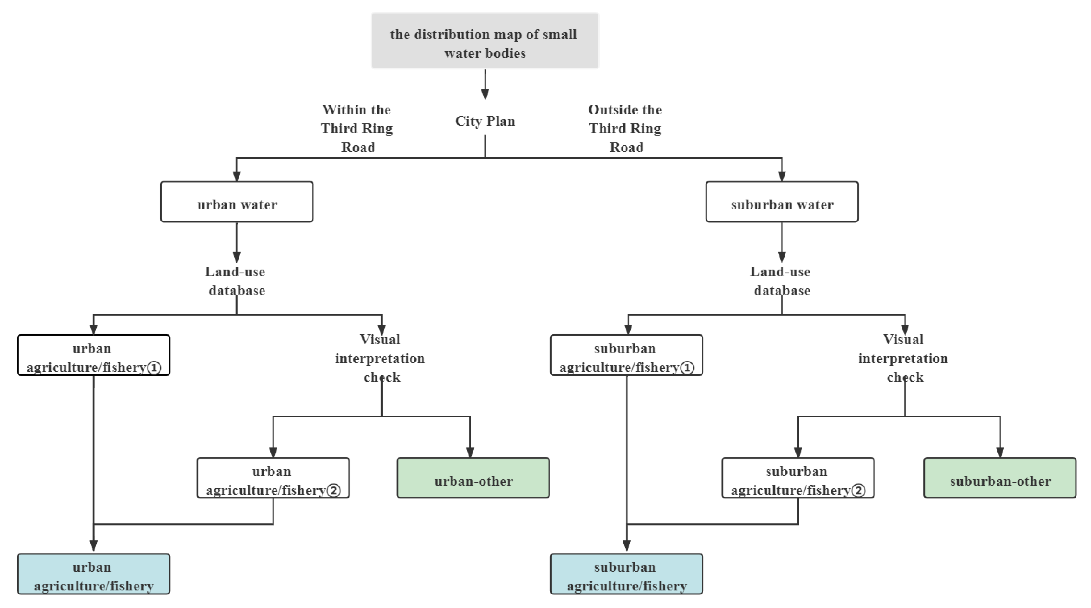
2.3. Sampling Design of in Situ Water Sample Collection
2.4. Water Quality Data
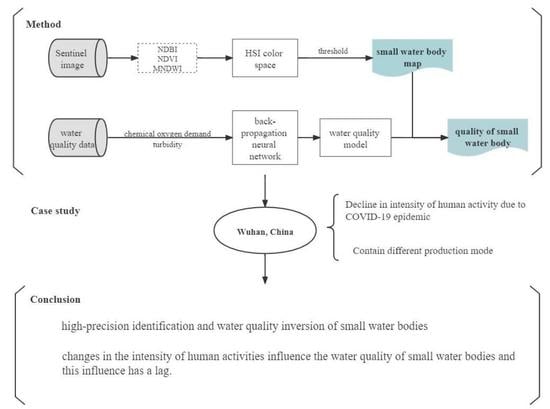
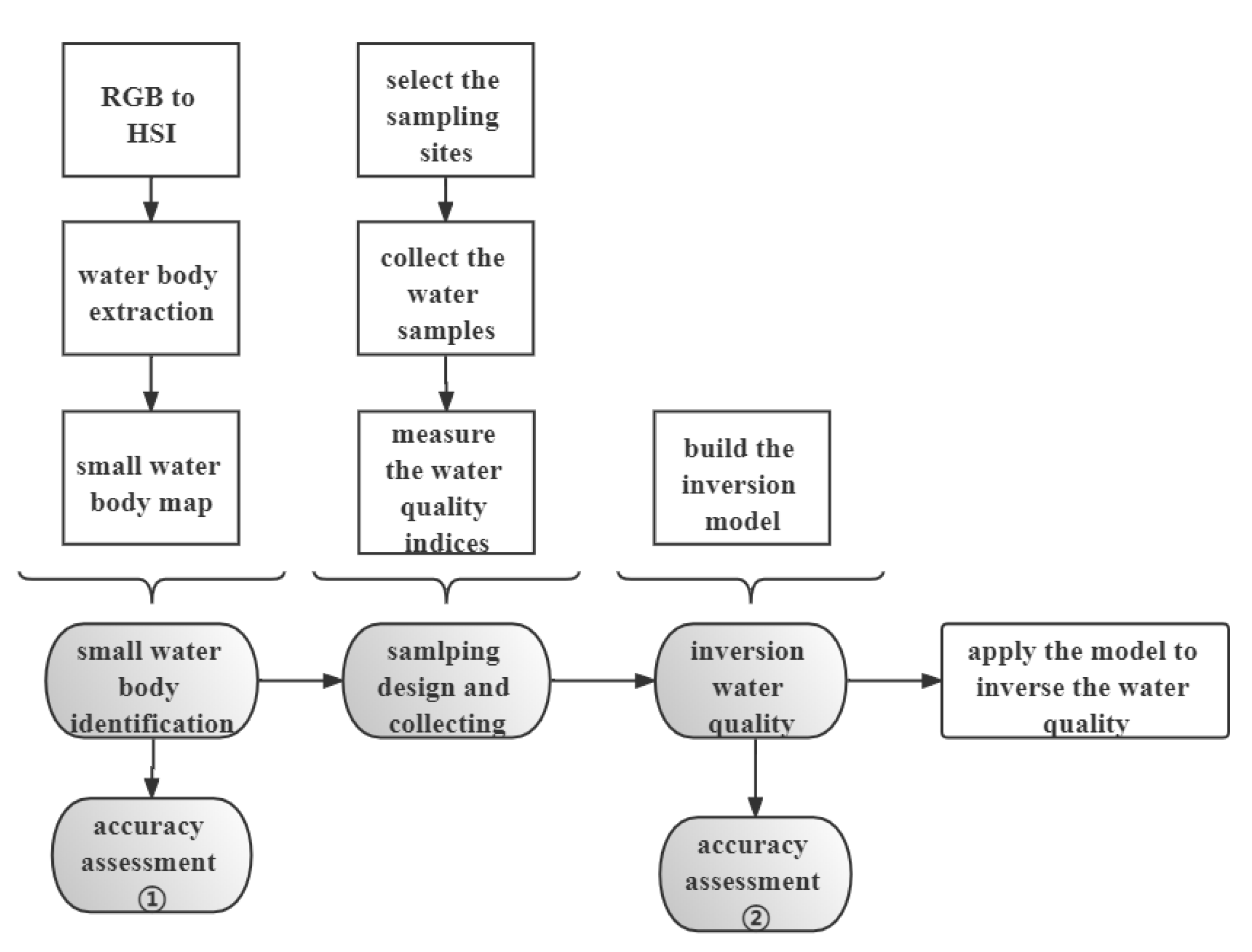
3. Method
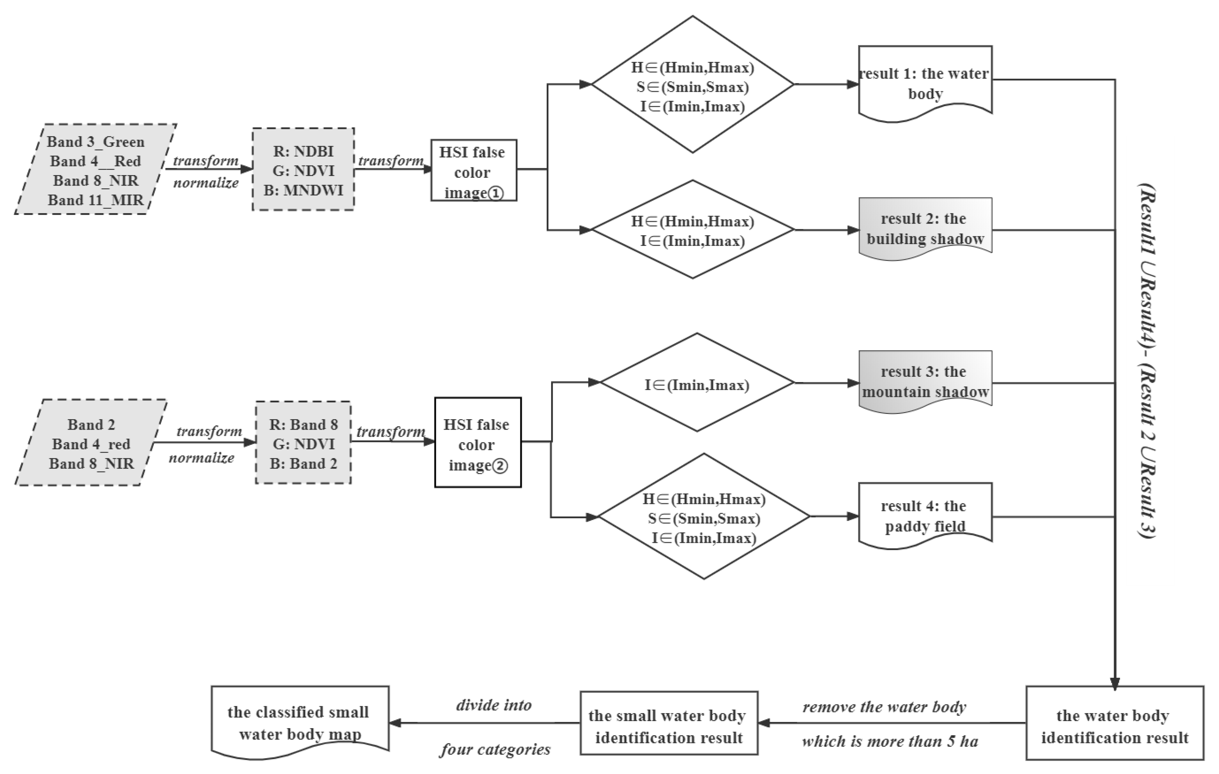
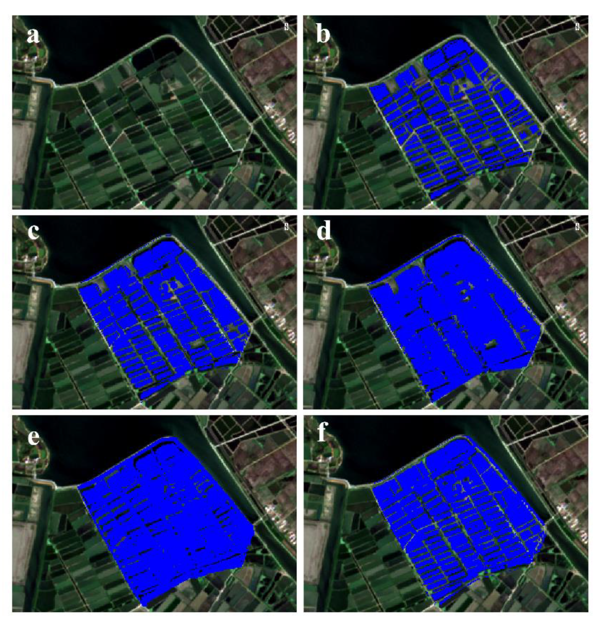
3.1. Small Waterbody Identification from Remote Sensing Images
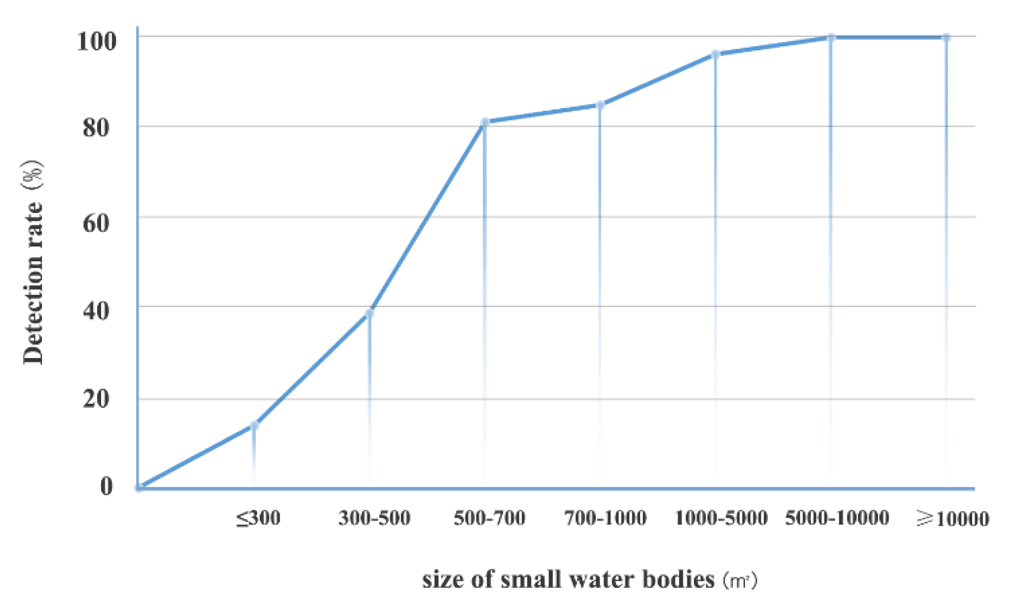
3.2. Accuracy Assessment of Small Waterbody Identification
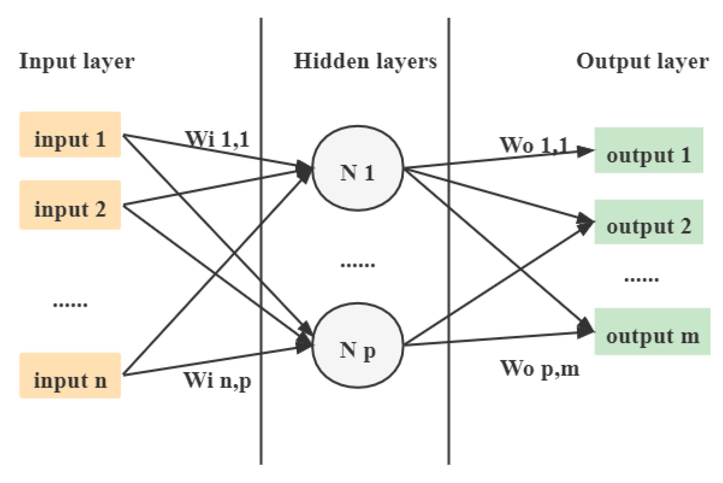
3.3. Water Quality Estimation from Remote Sensing Images
3.4. Accuracy Assessment of Water Quality Estimation
4. Results
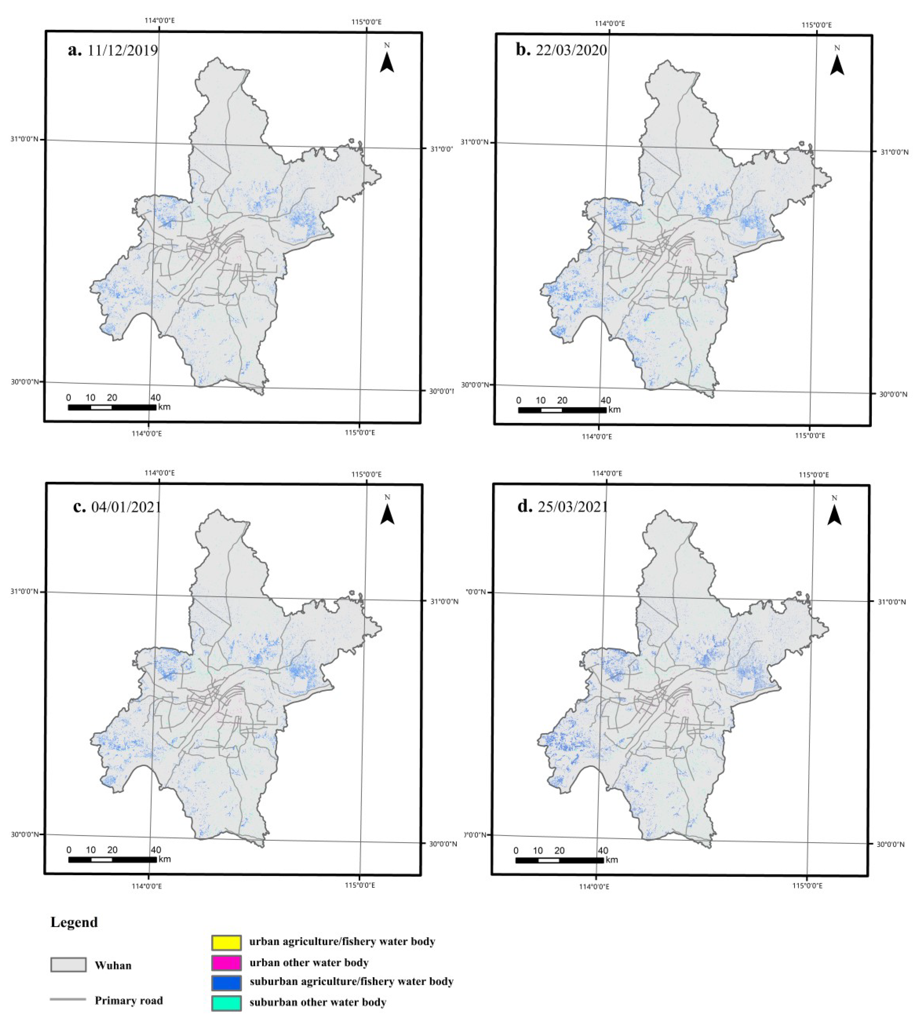
4.1. Small Water Body Identification
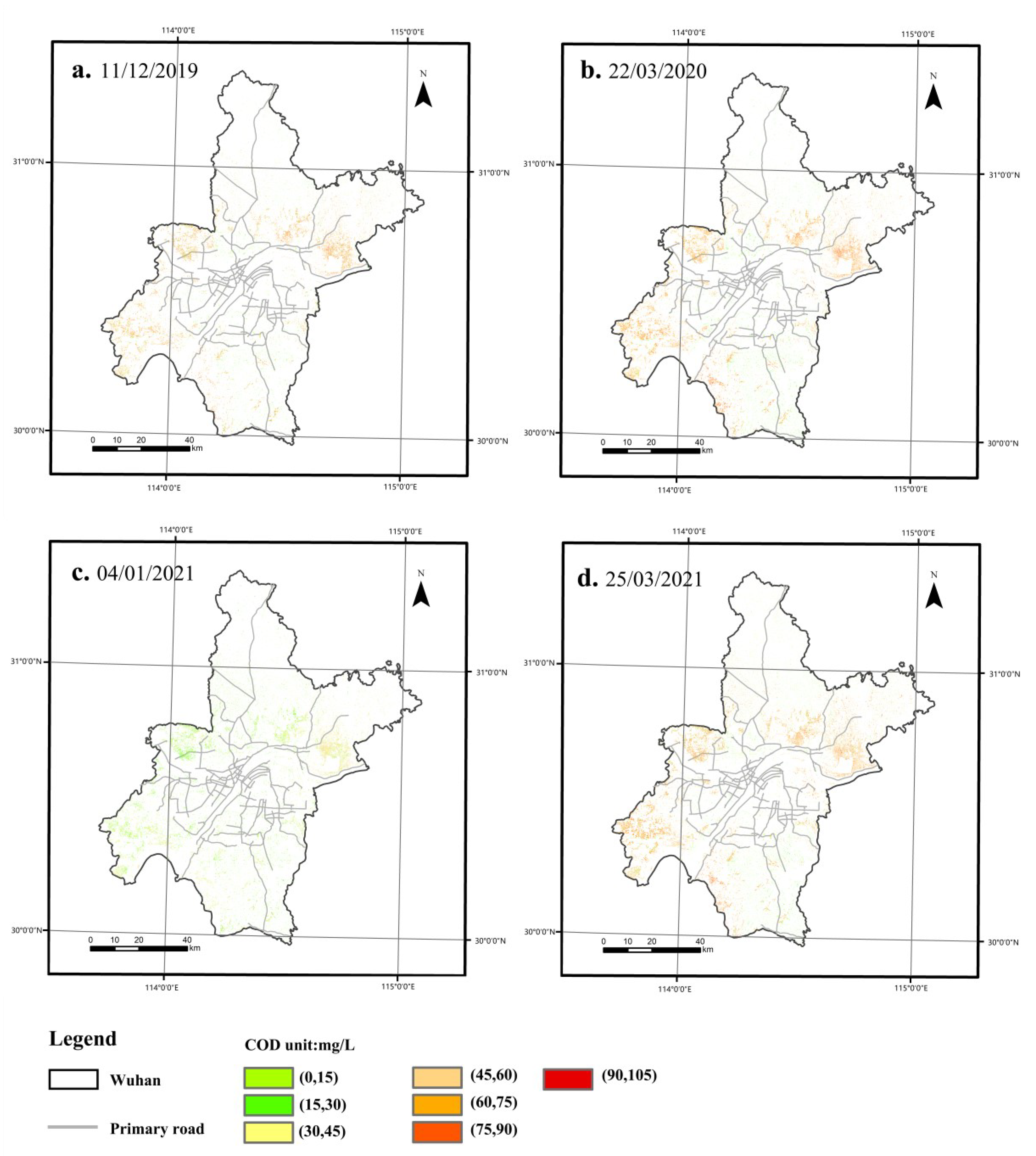
4.2. Water Quality Inversion
5. Discussion
5.1. HSI Color Space
5.2. BPNN
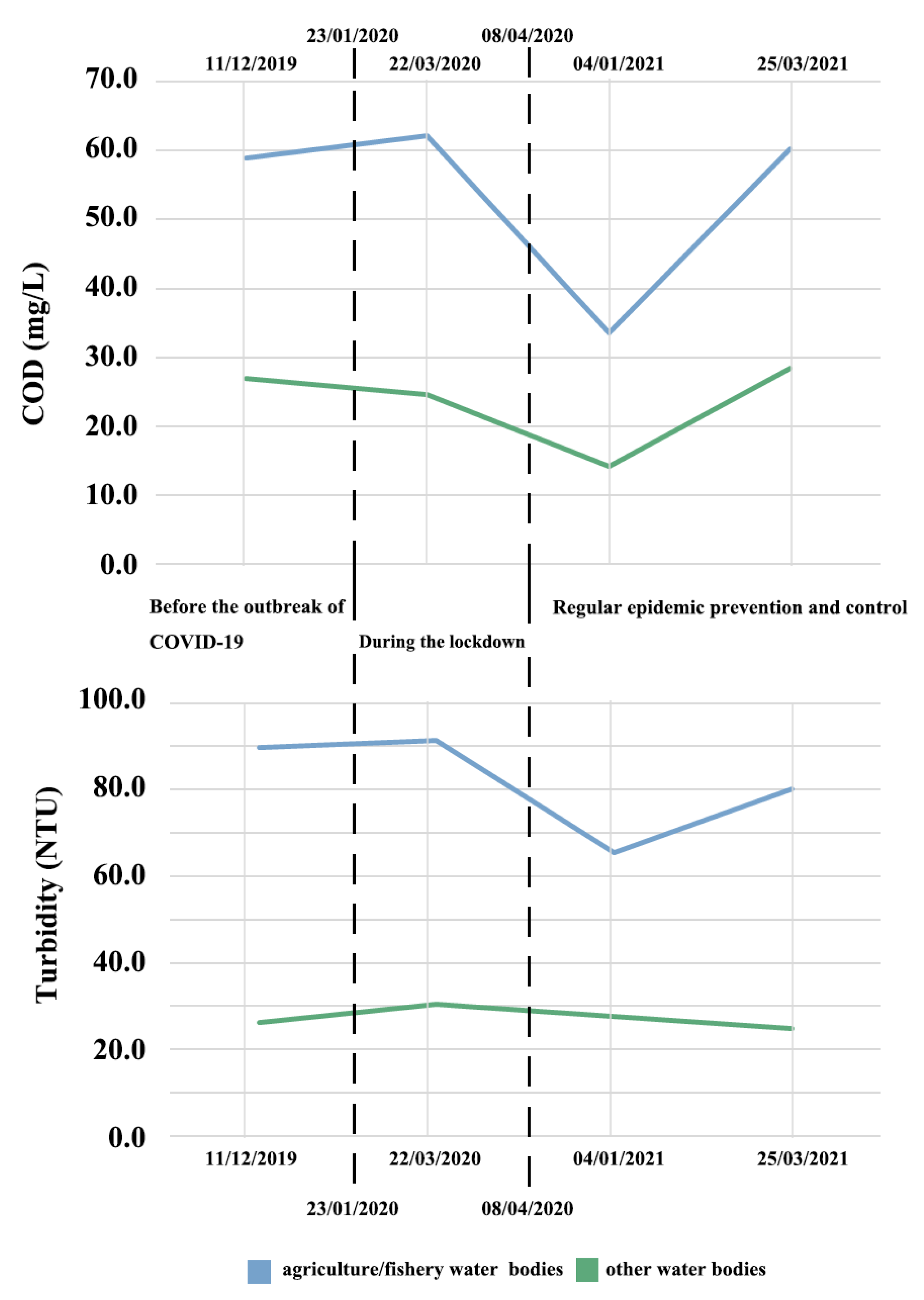
5.3. Water Quality Response to Intensity of Human Activities during COVID-19 Lockdown
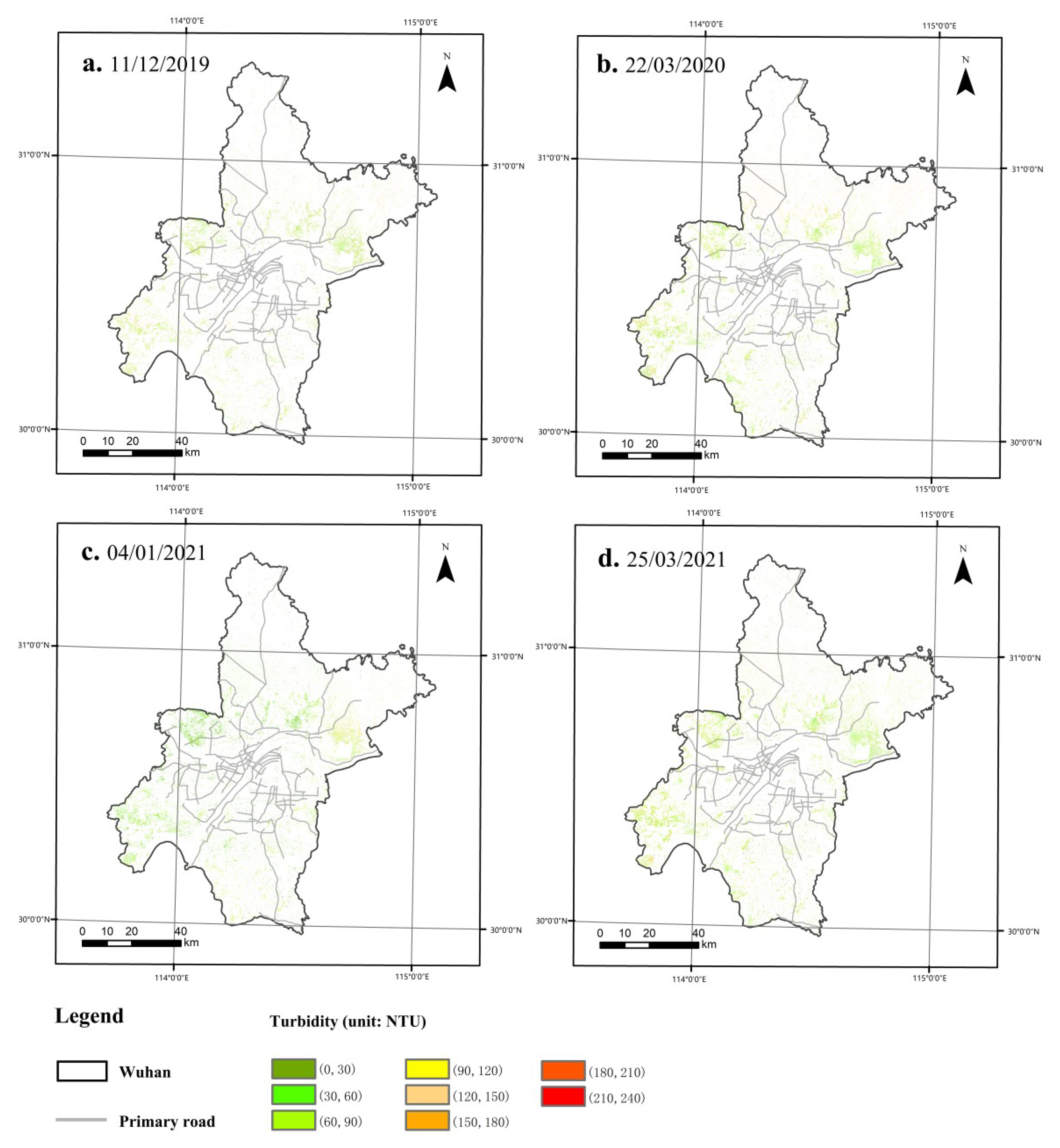
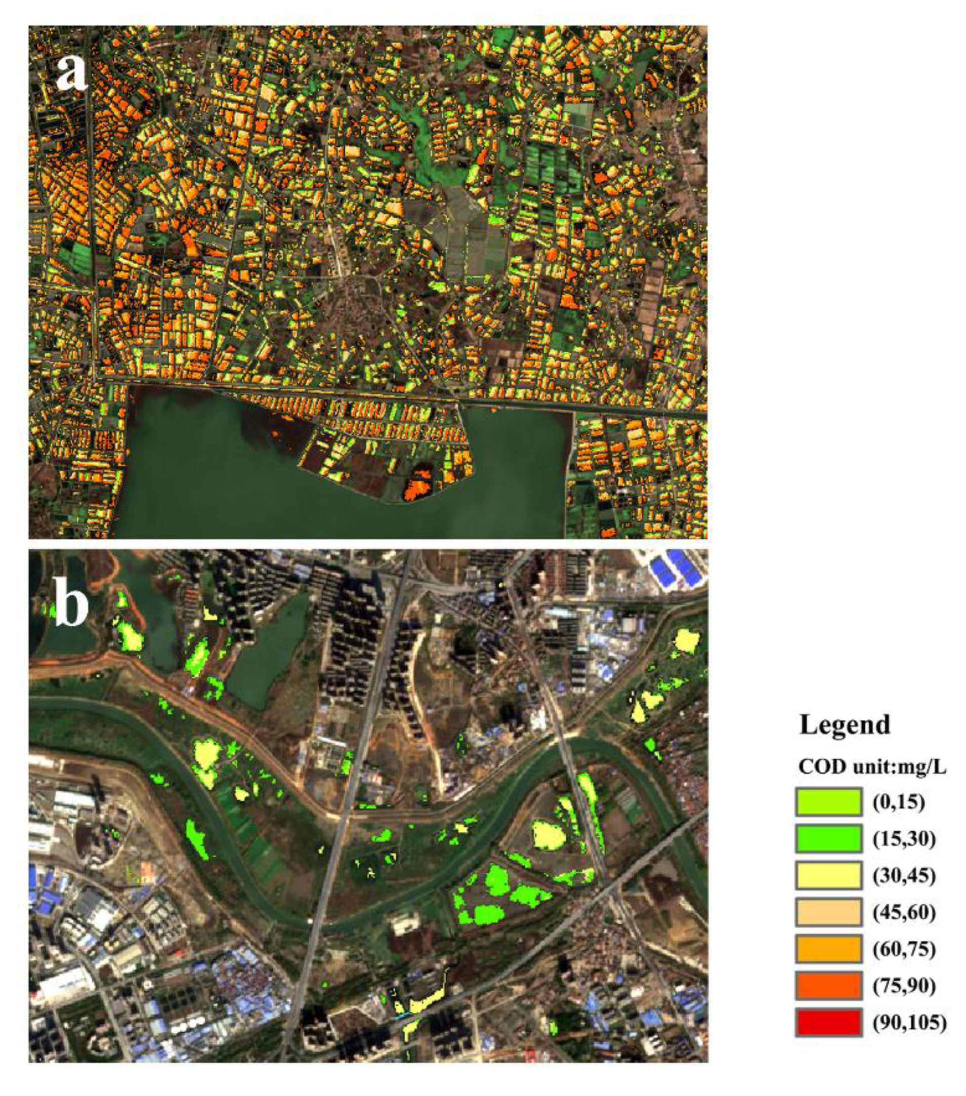
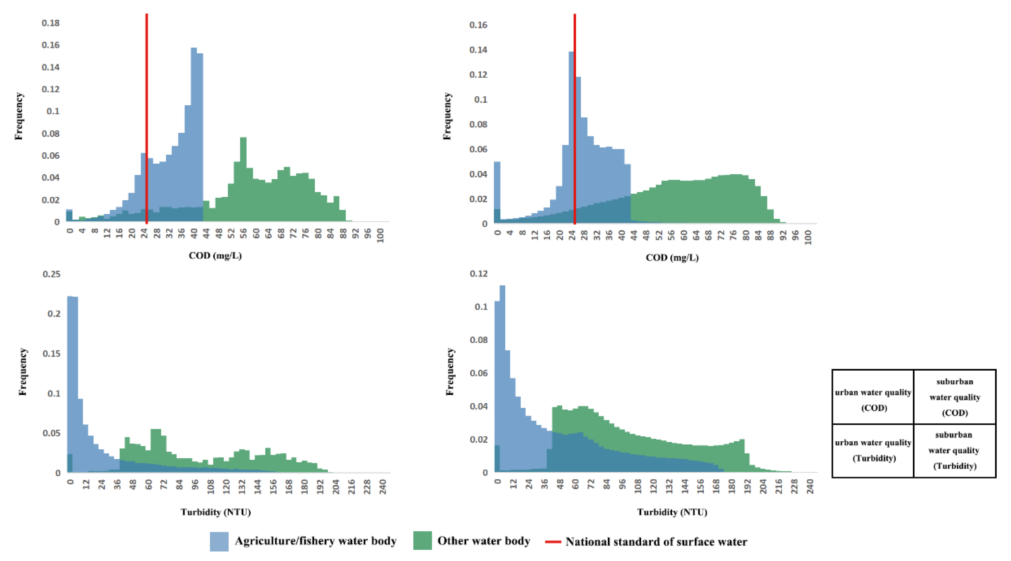
5.4. Spatial Variation in the Water Quality Due to COVID-19 Lockdown
5.5. Limitations and Further Study
6. Conclusions
Supplementary Materials
Author Contributions
Funding
Informed Consent Statement
Data Availability Statement
Conflicts of Interest
References
- Céréghino:, R.; Biggs, J.; Oertli, B.; Declerck, S. The ecology of European ponds: Defining the characteristics of a neglected freshwater habitat. Hydrobiologia 2008, 597, 1–6. [Google Scholar] [CrossRef]
- Meester, L.D.; Declerck, S.; Stoks, R.; Louette, G.; Brendonck, L. Ponds and pools as model systems in conservation biology, ecology and evolutionary biology. Aquat. Conserv. Mar. Freshw. Ecosyst. 2010, 15, 715–725. [Google Scholar] [CrossRef]
- Hackney, C.; Sumner, S. Distribution and Water as Related to Food Safety and Food Security. In Strategies for Achieving Food Security in Central Asia; Springer: Dordrecht, Germany, 2012; pp. 139–146. [Google Scholar]
- Landrigan, P.J.; Fuller, R.; Fisher, S.; Suk, W.A.; Sly, P.; Chiles, T.C.; Bose-O’Reilly, S. Pollution and children’s health. Sci. Total Environ. 2019, 650, 2389–2394. [Google Scholar] [CrossRef] [PubMed]
- Immerzeel, W.W.; Lutz, A.F.; Andrade, M.; Bahl, A.; Biemans, H.; Bolch, T.; Hyde, S.; Brumby, S.; Davies, B.J.; Elmore, A.C.; et al. Importance and vulnerability of the world’s water towers. Nature 2020, 577, 364–369. [Google Scholar] [CrossRef]
- McFeeters, S.K. The use of the normalized difference water index (NDWI) in the delineation of open water features. Int. J. Remote Sens. 1996, 17, 1425–1432. [Google Scholar] [CrossRef]
- Kloiber, S.M.; Brezonik, P.L.; Bauer, M.E. Application of Landsat imagery to regional-scale assessments of lake clarity. Water Res. 2002, 36, 4330–4340. [Google Scholar] [CrossRef]
- Xu, H. A Study on Information Extraction of Water Body with the Modified Normalized Difference Water Index (MNDWI). J. Remote Sens. 2005, 9, 589–595. [Google Scholar]
- Pei, Y.; Youjing, Z.; Yuan, Z. A Study on Information Extraction of Water System in Semi-arid Regions with the Enhanced Water Index (EWI) and GIS Based Noise Remove Techniques. Remote Sens. Inf. 2007, 6, 62–67. [Google Scholar] [CrossRef]
- Zhanfeng, S.; Liegang, X.; Junli, L.; Jiancheng, L.; Xiaodong, H. Automatic and high-precision extraction of rivers from remotely sensed images with Gaussian normalized water index. J. Image Graph. 2013, 18, 421–428. [Google Scholar]
- Mondejar, J.P.; Tongco, A.F. Near infrared band of Landsat 8 as water index: A case study around Cordova and Lapu-Lapu City, Cebu, Philippines. Sustain. Environ. Res. 2019, 29, 16. [Google Scholar] [CrossRef] [Green Version]
- Ding, Z.; Qi, N.; Dong, F.; Jinhui, L.; Wei, Y.; Shenggui, Y. Application of multispectral remote sensing technology in surface water body extraction. In Proceedings of the 2016 International Conference on Audio, Language and Image Processing (ICALIP), Shanghai, China, 11–12 July 2016; pp. 141–144. [Google Scholar]
- Zhou, X.; Marani, M.; Albertson, J.D.; Silvestri, S. Hyperspectral and Multispectral Retrieval of Suspended Sediment in Shallow Coastal Waters Using Semi-Analytical and Empirical Methods. Remote Sens. 2017, 9, 393. [Google Scholar] [CrossRef] [Green Version]
- Gordon, H.R.; Brown, O.B.; Jacobs, M.M. Computed relationships between the inherent and apparent optical properties of a flat homogeneous ocean. Appl. Opt. 1975, 14, 417–427. [Google Scholar] [CrossRef]
- Wu, G.; Cui, L.; Duan, H.; Teng, F.; Liu, Y. Absorption and backscattering coefficients and their relations to water constituents of Poyang Lake, China. Appl. Opt. 2011, 50, 6358–6368. [Google Scholar] [CrossRef]
- Wang, T.-S.; Tan, C.-H.; Chen, L.; Tsai, Y.-C. Applying Artificial Neural Networks and Remote Sensing to Estimate Chlorophyll-a Concentration in Water Body. In Proceedings of the 2008 2nd International Symposium on Intelligent Information Technology Application, Shanghai, China, 20–22 December 2008; pp. 540–544. [Google Scholar]
- Guang-jia, J.; Dian-wei, L.I.U.; Kai-shan, S.; Jing-ping, X.U.; Bai, Z.; Zong-ming, W. Estimation of Total Suspended Matter Concentration in Shitoukoumen Reservoir Based on a Semi-empirical Model. Remote Sens. Technol. Appl. 2010, 25, 107–111. [Google Scholar]
- Li, L.; Li, L.; Song, K. A Bio-optical Approach to Estimating Chlorophyll-a Concentration from Hyperspectral Remote Sensing. In Remote Sensing and Modeling of Ecosystems for Sustainability VII; Gao, W., Jackson, T.J., Wang, J., Eds.; SPIE: Bellingham, WA, USA, 2010; Volume 7809. [Google Scholar]
- Oga, T.; Umeki, Y.; Iwahashi, M.; Matsuda, Y.; IEEE. River water quality estimation based on convolutional neural network. In Proceedings of the 2018 Asia-Pacific Signal and Information Processing Association Annual Summit and Conference, Honolulu, Hawaii, 12–15 November 2018; pp. 1305–1308. [Google Scholar]
- Peterson, K.T.; Sagan, V.; Sloan, J.J. Deep learning-based water quality estimation and anomaly detection using Landsat-8/Sentinel-2 virtual constellation and cloud computing. GIScience Remote Sens. 2020, 57, 510–525. [Google Scholar] [CrossRef]
- Bie, W.; Fei, T.; Liu, X.; Liu, H.; Wu, G. Small water bodies mapped from Sentinel-2 MSI (MultiSpectral Imager) imagery with higher accuracy. Int. J. Remote Sens. 2020, 41, 7912–7930. [Google Scholar] [CrossRef]
- Matsushita, B.; Yang, W.; Chang, P.; Yang, F.; Fukushima, T. A simple method for distinguishing global Case-1 and Case-2 waters using SeaWiFS measurements. ISPRS J. Photogramm. Remote Sens. 2012, 69, 74–87. [Google Scholar] [CrossRef] [Green Version]
- Chung, S.-O.; Kim, H.-S.; Kim, J.S. Model development for nutrient loading from paddy rice fields. Agric. Water Manag. 2003, 62, 1–17. [Google Scholar] [CrossRef]
- Fang, Y.; Liu, G.; Tian, C.; He, X.; Song, G. Effect of Aquaculture Water Body Pollution on Breed Living Beings and the Recovery of Water Body. Res. Soil Water Conserv. 2005, 12, 198–200. [Google Scholar]
- Huang, X.; Wang, Y. Investigating the effects of 3D urban morphology on the surface urban heat island effect in urban functional zones by using high-resolution remote sensing data: A case study of Wuhan, Central China. ISPRS J. Photogramm. Remote Sens. 2019, 152, 119–131. [Google Scholar] [CrossRef]
- Ma, J.; Huang, S.; Xu, Z. Satellite remote sensing of lake area in Wuhan from 1973 to 2015. J. Hydraul. Eng. 2017, 48, 903–913. [Google Scholar] [CrossRef]
- Bherwani, H.; Nair, M.; Musugu, K.; Gautam, S.; Gupta, A.; Kapley, A.; Kumar, R. Valuation of air pollution externalities: Comparative assessment of economic damage and emission reduction under COVID-19 lockdown. Air Qual. Atmos. Health 2020, 13, 683–694. [Google Scholar] [CrossRef]
- Jakovljević, G.; Govedarica, M.; Álvarez-Taboada, F. Waterbody mapping: A comparison of remotely sensed and GIS open data sources. Int. J. Remote Sens. 2018, 40, 2936–2964. [Google Scholar] [CrossRef]
- Castillo, J.A.A.; Apan, A.A.; Maraseni, T.N.; Salmo, S.G. Estimation and mapping of above-ground biomass of mangrove forests and their replacement land uses in the Philippines using Sentinel imagery. ISPRS J. Photogramm. Remote Sens. 2017, 134, 70–85. [Google Scholar] [CrossRef]
- Sentinel-2_User_Handbook; 2015; Available online: https://sentinel.esa.int/documents/247904/685211/Sentinel-2_User_Handbook (accessed on 30 November 2020).
- Pałaś, K.W.; Zawadzki, J. Sentinel-2 Imagery Processing for Tree Logging Observations on the Białowieża Forest World Heritage Site. Forests 2020, 11, 857. [Google Scholar] [CrossRef]
- Gao, Y.; Zhang, X.; Tian, J.; Qian, J. Response of Water Quality in Shuangta Reservoir to Human Activities. Hydrology 2013, 33, 70–74. [Google Scholar]
- Ehlman, S.M.; Sandkam, B.A.; Breden, F.; Sih, A. Developmental plasticity in vision and behavior may help guppies overcome increased turbidity. J. Comp. Physiol. A 2015, 201, 1125–1135. [Google Scholar] [CrossRef] [Green Version]
- Cote, J.; Pilisi, C.; Morisseau, O.; Veyssiere, C.; Perrault, A.; Jean, S.; Blanchet, S.; Jacquin, L. Water turbidity affects melanin-based coloration in the gudgeon: A reciprocal transplant experiment. Biol. J. Linn. Soc. 2019, 128, 451–459. [Google Scholar] [CrossRef]
- Xu, J.; Jin, G.; Mo, Y.; Tang, H.; Li, L. Assessing Anthropogenic Impacts on Chemical and Biochemical Oxygen Demand in Different Spatial Scales with Bayesian Networks. Water 2020, 12, 246. [Google Scholar] [CrossRef] [Green Version]
- Sharaf El Din, E.; Zhang, Y.; Suliman, A. Mapping concentrations of surface water quality parameters using a novel remote sensing and artificial intelligence framework. Int. J. Remote Sens. 2017, 38, 1023–1042. [Google Scholar] [CrossRef]
- Mahvi, H.; Bazrafshan, E.; Jahed, G.R. Evaluation of COD Determination by ISO, 6060 Method, Comparing with Standard Method (5220, B). Pak. J. Biol. Sci. 2005, 8, 892–894. [Google Scholar] [CrossRef]
- Wang, G.; Wei, W. Uncertainties of COD Determination in Low Concentration Water Samples with Rapid Digestion Spectrophotometric Method. Environ. Sci. 2013, 38, 137–139. [Google Scholar]
- Wang, B.B.; Cao, M.H.; Zhu, H.D.; Chen, J.; Wang, L.L.; Liu, G.H.; Gu, X.M.; Lu, X.H. Distribution of perfluorinated compounds in surface water from Hanjiang River in Wuhan, China. Chemosphere 2013, 93, 468–473. [Google Scholar] [CrossRef] [PubMed]
- Lu, G.; Fei, B. Medical hyperspectral imaging: A review. J. Biomed. Opt. 2014, 19, 10901. [Google Scholar] [CrossRef] [PubMed]
- Zha, Y.; Gao, J.; Ni, S. Use of normalized difference built-up index in automatically mapping urban areas from TM imagery. Int. J. Remote Sens. 2010, 24, 583–594. [Google Scholar] [CrossRef]
- Huete, A.; Didan, K.; Miura, T.; Rodriguez, E.P.; Gao, X.; Ferreira, L.G. Overview of the radiometric and biophysical performance of the MODIS vegetation indices. Remote Sens. Environ. 2002, 83, 195–213. [Google Scholar] [CrossRef]
- Xu, H. Modification of normalised difference water index (NDWI) to enhance open water features in remotely sensed imagery. Int. J. Remote Sens. 2006, 27, 3025–3033. [Google Scholar] [CrossRef]
- Jiang, Z.; Qi, J.; Su, S.; Zhang, Z.; Wu, J. Water body delineation using index composition and HIS transformation. Int. J. Remote Sens. 2012, 33, 3402–3421. [Google Scholar] [CrossRef]
- Ouma, Y.O.; Tateishi, R. A water index for rapid mapping of shoreline changes of five East African Rift Valley lakes: An empirical analysis using Landsat TM and ETM+ data. Int. J. Remote Sens. 2006, 27, 3153–3181. [Google Scholar] [CrossRef]
- Feng, D. A new method for rapid extraction of water body information based on remote sensing data. Remote Sens. Technol. Appl. 2009, 24, 167–171. [Google Scholar]
- Guo, Z.-h.; Wu, J.; Lu, H.-y.; Wang, J.-z. A case study on a hybrid wind speed forecasting method using BP neural network. Knowl.-Based Syst. 2011, 24, 1048–1056. [Google Scholar] [CrossRef]
- Møller, M. A Scaled Conjugate Gradient Algorithm for Fast Supervised Learning. Neural Netw. 1993, 6, 525–533. [Google Scholar] [CrossRef]
- Vaart, A. Bayesian Regularization. In Proceedings of the International Congress of Mathematicians 2010 (ICM 2010), Hyderabad, India, 19–27 August 2010. [Google Scholar]
- Madsen, K.; Nielsen, H.B.; Tingleff, O. Methods for Non-Linear Least Squares Problems, 2nd ed.; Society for Industrial Applied Mathematics: Philadelphia, PA, USA, 2004. [Google Scholar]
- Ministry of Ecology and Environment of the PRC. Environmental quality standards for surface water. Implementation and monitoring of standards 2002. Available online: https://www.chinesestandard.net/PDF.aspx/GB3838-2002 (accessed on 30 November 2021).
- Zhang, Y.S.; Wu, L.; Ren, H.Z.; Deng, L.C.; Zhang, P.C. Retrieval of Water Quality Parameters from Hyperspectral Images Using Hybrid Bayesian Probabilistic Neural Network. Remote Sens. 2020, 12, 1567. [Google Scholar] [CrossRef]
- Benelli, G.; Govindarajan, M. Green-Synthesized Mosquito Oviposition Attractants and Ovicides: Towards a Nanoparticle-Based “Lure and Kill” Approach? J. Clust. Sci. 2017, 28, 287–308. [Google Scholar] [CrossRef]

| Index | Formula | Representative Element |
|---|---|---|
| NDBI | Soil or building | |
| NDVI | Vegetation | |
| MNDWI | Water |
| Hue | Saturation | Intensity |
|---|---|---|
| Phase Results | Threshold of H | Threshold of S | Threshold of I |
|---|---|---|---|
| Result 1 | (210,270) | (0.025,1) | (0.5,1) |
| Result 2 | (0,190) | - | (0,0.51) |
| Result 3 | - | - | (0.28,1) |
| Result 4 | (115,360) | (0,73,1) | (0,0.35) |
| Method | Formula | Reference Number |
|---|---|---|
| NDWI | [5] | |
| NDWI3 | [45] | |
| EWI | [46] | |
| MNDWI | [7] |
| HSI | EWI | MNDWI | ndwi3 | NDWI | |
|---|---|---|---|---|---|
| OA | 0.980 | 0.832 | 0.778 | 0.793 | 0.746 |
| UA | 0.995 | 0.772 | 0.711 | 0.740 | 0.680 |
| PA | 0.967 | 0.971 | 0.981 | 0.940 | 0.985 |
| K | 0.959 | 0.657 | 0.542 | 0.575 | 0.477 |
| Date | Water Area (km2) | Small Water Area (km2) | Other Water Body (km2) | Agriculture/Fishery Water Body (km2) | ||
|---|---|---|---|---|---|---|
| Urban | Suburban | Urban | Suburban | |||
| 11/12/2019 | 1129.32 | 225.32 | 2.93 | 40.25 | 0.26 | 181.58 |
| 22/03/2020 | 1293.22 | 306.08 | 3.21 | 52.20 | 0.33 | 250.35 |
| 04/01/2021 | 1268.02 | 279.86 | 4.61 | 51.73 | 0.28 | 223.23 |
| 25/03/2021 | 1295.99 | 324.84 | 3.57 | 57.29 | 0.26 | 263.72 |
| Training Algorithm | ||||
|---|---|---|---|---|
| water turbidity | agriculture/fishery water body | Levenberg–Marquardt | 0.9390 | 0.8782 |
| Bayesian regularization | 0.7636 | 0.6782 | ||
| Scaled conjugate gradient | 0.8694 | 0.5315 | ||
| other water body | Levenberg–Marquardt | 0.8081 | 0.8119 | |
| Bayesian regularization | 0.6443 | 0.7224 | ||
| Scaled conjugate gradient | 0.7194 | 0.6808 | ||
| COD | agriculture/fishery water body | Levenberg–Marquardt | 0.9215 | 0.6699 |
| Bayesian regularization | 0.9015 | 0.8679 | ||
| Scaled conjugate gradient | 0.8944 | 0.9586 | ||
| other water body | Levenberg–Marquardt | 0.8680 | 0.8753 | |
| Bayesian regularization | 0.9001 | 0.4205 | ||
| Scaled conjugate gradient | 0.6484 | 0.1874 |
Publisher’s Note: MDPI stays neutral with regard to jurisdictional claims in published maps and institutional affiliations. |
© 2022 by the authors. Licensee MDPI, Basel, Switzerland. This article is an open access article distributed under the terms and conditions of the Creative Commons Attribution (CC BY) license (https://creativecommons.org/licenses/by/4.0/).
Share and Cite
Wang, L.; Bie, W.; Li, H.; Liao, T.; Ding, X.; Wu, G.; Fei, T. Small Water Body Detection and Water Quality Variations with Changing Human Activity Intensity in Wuhan. Remote Sens. 2022, 14, 200. https://doi.org/10.3390/rs14010200
Wang L, Bie W, Li H, Liao T, Ding X, Wu G, Fei T. Small Water Body Detection and Water Quality Variations with Changing Human Activity Intensity in Wuhan. Remote Sensing. 2022; 14(1):200. https://doi.org/10.3390/rs14010200
Chicago/Turabian StyleWang, Lingjun, Wanjuan Bie, Haocheng Li, Tanghong Liao, Xingxing Ding, Guofeng Wu, and Teng Fei. 2022. "Small Water Body Detection and Water Quality Variations with Changing Human Activity Intensity in Wuhan" Remote Sensing 14, no. 1: 200. https://doi.org/10.3390/rs14010200
APA StyleWang, L., Bie, W., Li, H., Liao, T., Ding, X., Wu, G., & Fei, T. (2022). Small Water Body Detection and Water Quality Variations with Changing Human Activity Intensity in Wuhan. Remote Sensing, 14(1), 200. https://doi.org/10.3390/rs14010200