Abstract
Over the last decade, a 3D reconstruction technique has been developed to present the latest as-is information for various objects and build the city information models. Meanwhile, deep learning based approaches are employed to add semantic information to the models. Studies have proved that the accuracy of the model could be improved by combining multiple data channels (e.g., XYZ, Intensity, D, and RGB). Nevertheless, the redundant data channels in large-scale datasets may cause high computation cost and time during data processing. Few researchers have addressed the question of which combination of channels is optimal in terms of overall accuracy (OA) and mean intersection over union (mIoU). Therefore, a framework is proposed to explore an efficient data fusion approach for semantic segmentation by selecting an optimal combination of data channels. In the framework, a total of 13 channel combinations are investigated to pre-process data and the encoder-to-decoder structure is utilized for network permutations. A case study is carried out to investigate the efficiency of the proposed approach by adopting a city-level benchmark dataset and applying nine networks. It is found that the combination of IRGB channels provide the best OA performance, while IRGBD channels provide the best mIoU performance.
1. Introduction
Over the last decade, the concept of city information modelling (CIM) has received a growing interest in many fields, such as surveying engineering and civil engineering [1]. Generally, CIM provides valuable benefits for stakeholders, including enhancing the public management process and establishing an intelligent digital platform to store, control, and understand big data. Xu et al. [2] suggested that geographic information systems (GIS) and building information modelling (BIM) can be integrated to facilitate and achieve the CIM concept. GIS models are utilized to represent graphical and geometrical information, while BIM models are applied to characterize semantic and topological information. Nonetheless, issues of model accuracy and timely information update are challengeable [3]. Furthermore, it is challenging to automatically identify the discrepancies between the as-built and as-planned models, which would cause significant delays, for example, in responding to project modification management [4,5].
A popularly used technique to create the as-built model is the 3D reconstruction, which has been developed to present the latest as-is information for infrastructures and the city. To acquire the point cloud data, laser scanning technologies such as light detection and ranging (LiDAR), terrestrial laser scanning system (TLS), and aerial laser scanning system (ALS) have been usually adopted. Many studies have presented that the main advantages of the TLS technologies include high point density (about one billion points per scan) and high geometric accuracy (up to millimeters) [6,7]. Therefore, TLS is more appropriate for CIM applications (requires high accuracy and density data). In addition, unlike the data collected in the typical remote sensing applications (e.g., satellite images and ALS), the TLS can collect image information of the scene immediately after completing the laser scanning. With the coordinate transformation matrix (usually provided by the manufacturer), the color information (RGB) can be directly mapped to the corresponding laser point. In this case, the data obtained through TLS usually has seven aligned channels of data: RGB from the camera sensor and XYZ and I (intensity).
After acquiring raw point clouds that can provide accurate geometric information for CIM, the semantic segmentation technique is usually adopted to obtain the semantic information from the raw point cloud. In addition to the seven channels in the raw point cloud, additional channels can be derived to describe the scene. The widely used two types are the depth channel and the normal vector channel generated by XYZ. However, in practice, not all channels can bring a positive improvement to semantic segmentation. Several studies in the remote sensing application have indicated the importance of selecting an optimal combination of data channels regarding multispectral datasets. For instance, Yang et al. [8] presented a novel hyperspectral band approach to select an optimal band for image classification based on clustering-based selection methods. Their results indicated that the proposed method was more effective and able to generate better band selection results. Li et al. [9] utilized discrete particle swarm optimization to model the various errors (i.e., reconstruction, imaging, and demosaicing errors) associated with spectral reconstruction for optimal channel combination. The optimization results reduced the time in the computational process. Abdalla et al. [10] developed a robust DL method to group the RGB channels for automatic color calibration for plants. Bhuiyan et al. [11] experimented with testing the optimal three-channel combination in model prediction using very high spatial resolution (VHSR) multispectral (MS) satellite images. Their findings emphasized the importance of considering input MS channels and the careful selection of optimal channels of DL network predictions for mapping applications. Park et al. [12] presented a novel image prioritization method to select the limited channel based on cloud coverage for nanosatellite application. By reducing the channels, they achieved an extremely low computational power and light network on a nanosatellite.
The abovementioned studies have provided insightful guidance for optimal channel combinations for image channels. However, these researches mainly investigated the optimal combination of channels in land-use mapping, agricultural, and disaster monitoring, focusing on the region highlight field (e.g., ice-wedge polygons). There is no agreement on the optimal combination of channels that should be used for CIM applications in urban scenes. For example, Pierdicca et al. [13] presented the deep learning (DL) framework using 12 channels as input: XYZ coordinates, X’Y’Z’ normalized coordinates, color features (HSV channels), normal features (in X, Y, and Z direction) for cultural heritage point cloud segmentation. Alshawabkeh [14] developed a novel dataset to evaluate the feasibility of combined LiDAR data and images for object segmentation by integrating RGB-D channels (i.e., color and depth information). In the joint 3D object detection and semantic segmentation, Meyer et al. [15] used RGB together with aligned LiDAR information (point’s range, height, azimuth angle, intensity, and indication of occupation) as the input of their networks. Lawin et al. [16] transformed the XYZ channels into depth and normal information and particularly investigated the improvements in 3D semantic segmentation by using the depth, color, and normal information.
Thus, the present paper aims to explore a simple optimal combination of data channels based on their semantic segmentation performance in the urban scenario. To more objectively evaluate the gain from the combination of channels, the performance of various channel combinations will be tested on different published encoder-to-decoder segmentation networks in this study. Objectives are set to accomplish the aim as follows: (1) To determine the optimal group of channels in terms of its overall accuracy (OA) and mean intersection over union (mIoU); and (2) to empirically verify the robustness of the optimal channel combination across different networks.
The remainder of this paper is organized as follows. The second section will introduce the selected benchmark dataset and the proposed framework and experiment arrangement for the optimal channel combination selection. Then, the performance of various channel combinations on different networks is summarized in the third section. Findings are drawn in the fourth section and the final section.
2. Materials and Methodology
2.1. Paradigms for Semantic Segmentation
According to the comprehensive survey proposed by Guo et al. [17], point cloud semantic segmentation approaches in the DL framework can be divided in three paradigms: Projection-based, point-based, and discretization-based. The projection-based methods usually project a 3D point cloud into 2D images, including multi-view and spherical images. The point-based methods directly work on irregular point clouds by applying dedicated local features convolutions. The discretization-based methods usually convert a point cloud into volumetric rasterization to create an ordered grid of point clouds.
The point-based and discretization-based approach is directly processed on the 3D data, which is extremely time-consuming or memory-costly in sampling training and inferencing. For example, in the work of RandLA-Net [18], they evaluate the time consumption of recent representative works on the Sequence 08 of the SemanticKITTI with 81,920 total number of points, where the best test result was 442 points/s. On the contrary, the SnapNet [19] test 30 M points used even worse arithmetic. The average processing time is about 32 min, and the corresponding process speed is about 15,625 points/s, which is 35 times faster than the point-based method. Meanwhile, for the CIM application, the total number of points is up to 108 per scan. Therefore, the point-based and discretization-based approaches are not efficient enough in terms of time. On the other hand, the performance of multi-view segmentation methods is dependent on viewpoint selection and occlusions. Therefore, in the present paper, spherical images-based semantic segmentation is adopted.
2.2. Study Materials
The online large-scale point cloud segmentation benchmark dataset Semantic3D is used in this case study [20]. This benchmark dataset contains 15 annotated point clouds representing different city scenes, where the points are labelled as eight classes (i.e., 1: Man-made terrain, 2: Natural terrain, 3: High vegetation, 4: Low vegetation, 5: Buildings, 6: Hard scape, 7: Scanning artefacts, 8: Cars). Each point cloud is obtained by a separate scanning. The basic information of 15 labelled point clouds is summarized in Table 1.

Table 1.
Summary of basic information of 15 labelled point clouds.
2.3. Methodology
The way to select the optimal group of data channels for semantic segmentation consists of two parts: Data preprocessing and two-step verification.
In the data preprocessing stage, which is shown in Figure 1, the first step is to convert the data of different channels in the point clouds into a panoramic (PAN) image separately. The next step is to slip the PAN image into subsets. The data in the panoramic form usually have a large resolution. For example, PAN image resolution for a normal-scale single laser scan station with around thirty million laser points can be higher than 3000 x 7200. Such a large resolution requires a high graphic memory size for the hardware. The PAN form data need to be split into pieces with smaller sizes according to the hardware performance. The PAN images are augmented by random cropping with 512 x 512 and random horizontal flipping.

Figure 1.
Detailed steps of the data preprocess.
Additionally, for the laser data in CIM, the “invalid” data often occurs. When the emitted laser beam points to the sky and does not return, there would be no valid coordinates and intensity, as a result, “zero” appears in the dataset. Therefore, to accelerate the convergence speed of neural network training, the proportion of such anomalous data in the comprehensive data is required to be adjusted.
Before grouping the data from different channels into different combinations, the image entropy () for each channel should be calculated [21]. Entropy is a statistical measure of randomness that can be used to characterize the texture or the contained information of the input image. The entropy of an image can be calculated by the first order from its histogram which provides the occurrence frequency (or probability) of all different grey levels in the image. The first-order image entropy is calculated as follows, where is the probability of grey level :
Using the entropy, those possible channels that are richer in information can be roughly determined. Therefore, in the subsequent channel grouping, some meaningless combinations are targeted and filtered out so as to reduce the time for choosing the optimal channel combination. In the channel grouping, the R, G, and B channels from the image are integrated with the I (intensity) channel acquired by the laser scanner to investigate the effect of intensity on semantic segmentation results. Alternatively, the R, G, and B channels from the image can be combined with the X, Y, and Z channels from the laser scanner, respectively, to compare the performance gained from the different channels. After that, the datasets for semantic segmentation are prepared, and all the images with appropriate sizes are stored according to the predefined combinations.
In selecting the optimal channel combination, a two-step verification strategy is applied to speed up identifying potential optimal combinations. First, networks with fewer parameters are applied to quickly estimate the potential optimal channel combinations. Then, networks with the deeper structure are adopted to verify the robustness of the optimal channel combinations. If the results show a high consistency across all the different networks, a reliable basis can be achieved for further subsequent substitutions or changes to the neural networks.
The encoder-to-decoder architecture for semantic segmentation is applied in this research. The encoder generates the feature maps for the input image, while the decoder uses the learned deconvolution layers to recover the image to the original size from the feature maps. The encoder-to-decoder structure can achieve better performance in reducing the information loss problem than those of the fully convolutional structure [22]. In addition, the structure of encoder-to-decoder is more flexible, as the encoder and decoder can be chosen from the commonly used neural network structures, respectively. For example, the encoder can be chosen from the ResNet, MobileNet, and Xception [23,24,25]. The performance of different neural networks with varying complexity are evaluated in terms of overall accuracy (OA) and mean intersection over union (mIoU).
2.4. Experiment Arrangement
It is necessary to ensure that the test data is similar to the data used for network training [26]. Therefore, the selection of test data is based on the following reasons. First, it is noticed that point clouds 1–3, point clouds 4–6, and point clouds 8–9 are collected from three city scenes, respectively. Hence, a random point cloud from each scene is selected as the test data (i.e., point clouds 2, 5, and 8). Since the remaining 6 point clouds (i.e., point clouds 9–15) are collected from six different city scenes, to keep the test-to-train ratio similar to the previous selection (around 1/3), two point clouds (i.e., point clouds 9 and 12) are randomly selected as the test data. Therefore, a total of five labelled point clouds were selected for testing, and the remaining ten are used to train the semantic segmentation networks, as shown in Table 1.
The preprocessing of the dataset follows the proposed method demonstrated in Section 2, where the size of the input images is taken as 512 × 512 to contain enough context information for semantic segmentation. Before deciding the combination of channels, it is necessary to check the image entropy first to avoid the combination with very little information.
As indicated in Figure 2, among the 15 scans provided by the Semantic 3D, the entropy values of RGB tend to be consistent. All of them remain in the top three, followed by intensity, but the performance is not stable for the other four channels (X, Y, Z, D). Therefore, the RGB channels from the image sensor dominate the subsequent channel combinations. Moreover, to verify the improvement of the data from the laser scanning on the semantic segmentation, the remaining channels are combined with RBG separately.
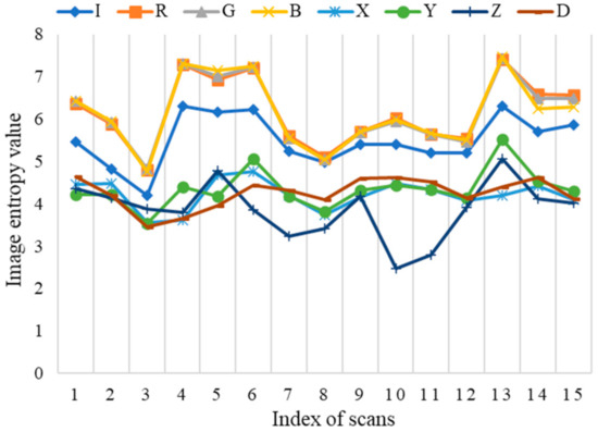
Figure 2.
The entropy of different channel data.
As shown in Table 2, a total of 13 combinations of channels are investigated in this research. These combinations are designed to investigate the effect of channels X, Y, Z, D, and intensity on the segmentation performance. Nine popular networks are used in this study, which include two basic U-net with different depths, seven networks having the same decoder (i.e., DeepLab v3+), and different backbones (i.e., ResNet18, ResNet50, ResNet101, MobileNetV2, Xception, Inception-ResNet-v2, HRCNet). All the structures of networks are the same as the original implementation, and detailed network structures refer to [25,27,28]. Finally, the cross-entropy loss is used in this study.

Table 2.
Combinations of channels.
The experiment is carried out on a PC with a processor of AMD Ryzen 9 3950X, RAM of 64 GB, and two GPUs of NVIDIA GeForce GTX 2080Ti. In addition, MATLAB 2020b is used for programming on the operating system of Windows 10. For a fair comparison through the whole experiment process, all the training used the same training protocol, which is a widely used strategy in deep learning research [29,30,31]. More specifically, the SGD optimizer with a base learning rate of 0.05, a momentum of 0.9, and a weight decay of 0.001 was adopted in this study. The step learning rate policy was applied, which drops the learning rate by a factor of 0.1 every 10 epochs. For data augmentation, random image extraction and random horizontal flipping were applied (as described in the data process step). The total number of augmented images was 384 K, which were divided into 50 groups for training (50 epochs). Due to the limited physical memory on GPU cards, the “batchsize” was set as 16 (a total of 24 K iteration), and synchronized batch normalization across GPU cards was adopted during training. Similar with [29,30,31], by applying random data augmentation and batch normalization, all the networks used in this study are considered to be resistant to overfitting.
3. Results
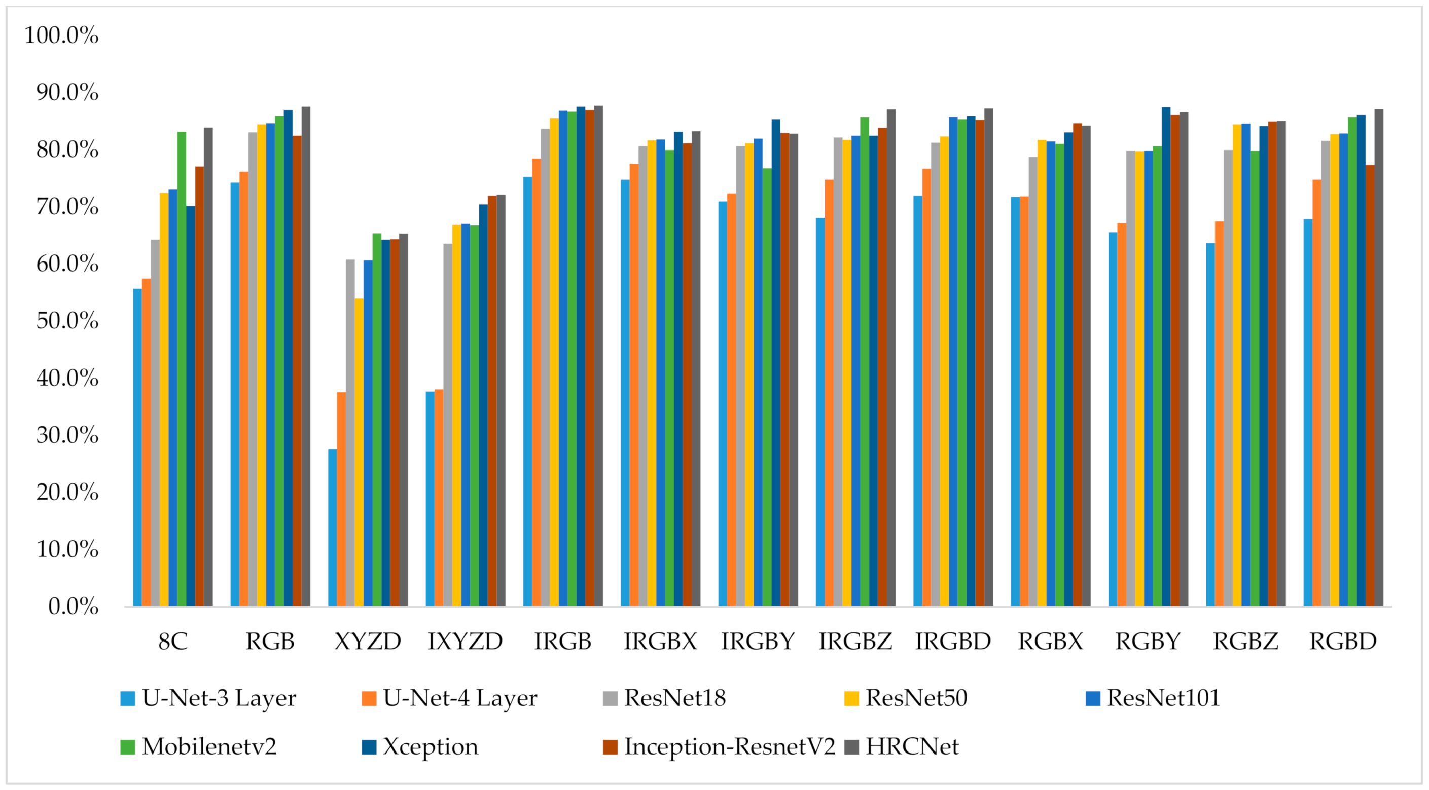
Figure 3 and Figure 4 demonstrate the mIoU and OA performance of the 13 combinations using nine networks. It is found that only the intensity channel brings a stable improvement of the segmentation performance. As shown in Table 3, the intensity channel improves mIoU and OA by an average of 3.24% and 2.01%, respectively. In contrast, it is found that the X, Y, and Z channels impair the segmentation performance. Table 3 shows that the X, Y, and Z channels reduce the mIoU by 2.84%, 2.97%, and 0.63%, respectively, and reduce the OA by 2.69%, 4.05%, and 3.46%, respectively. Finally, it is found that the effect of D channel depends on the criteria used for performance evaluation. More specifically, an additional channel of distance improves the mIoU by 3.09%, while reduces the OA by 2.0%. Since mIoU represents the average of the segmentation accuracy of each class, which indicates that the D channel is beneficial for the segmentation of imbalanced classes (classes with less data, i.e., difficult for segmentation).
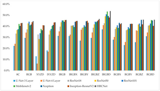
Figure 3.
Mean intersection over union (mIoU) on test point clouds.
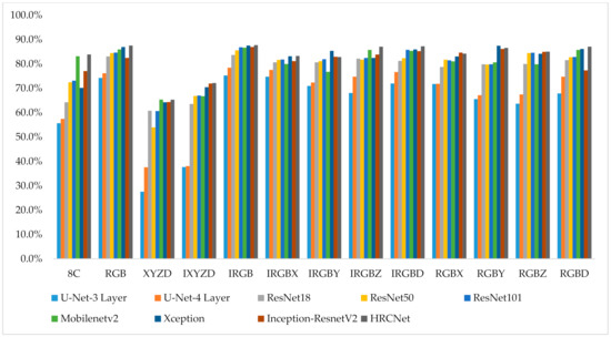
Figure 4.
Overall accuracy (OA) on test point clouds.

Table 3.
Average improvement by adding different channels.
4. Discussion
Based on the aforementioned results, it is inferred that the combination of IRGBD channels provides the best mIoU performance, while the combination of IRGB channels provides the best OA performance. These inferences are confirmed in Table 4 and Table 5, where the highest value of mIoU and OA for each network is highlighted as green and yellow, respectively. It is observed that the optimal combination of channels is the same for all networks, which shows the robustness of the optimal combination.

Table 4.
The mIoU of seven networks regarding different combinations of channels (the highest mIoU for each network is marked as green).

Table 5.
OA of seven networks regarding different combinations of channels (the highest OA for each network is marked as yellow).
In the meantime, by ranking the mIoU and OA of all the 13 channel combinations for seven networks, as shown in Table 6 and Table 7, it is found that the worst channel combination also presents a high consistency across the seven networks, but the consistency decreases for other combinations ranked in the middle. This indicates that the channel combinations with respect to extreme cases are more consistent than others.

Table 6.
Ranking of the mIoU performance of 13 channel combinations for seven networks.

Table 7.
Ranking of the mIoU performance of 13 channel combinations for seven networks.
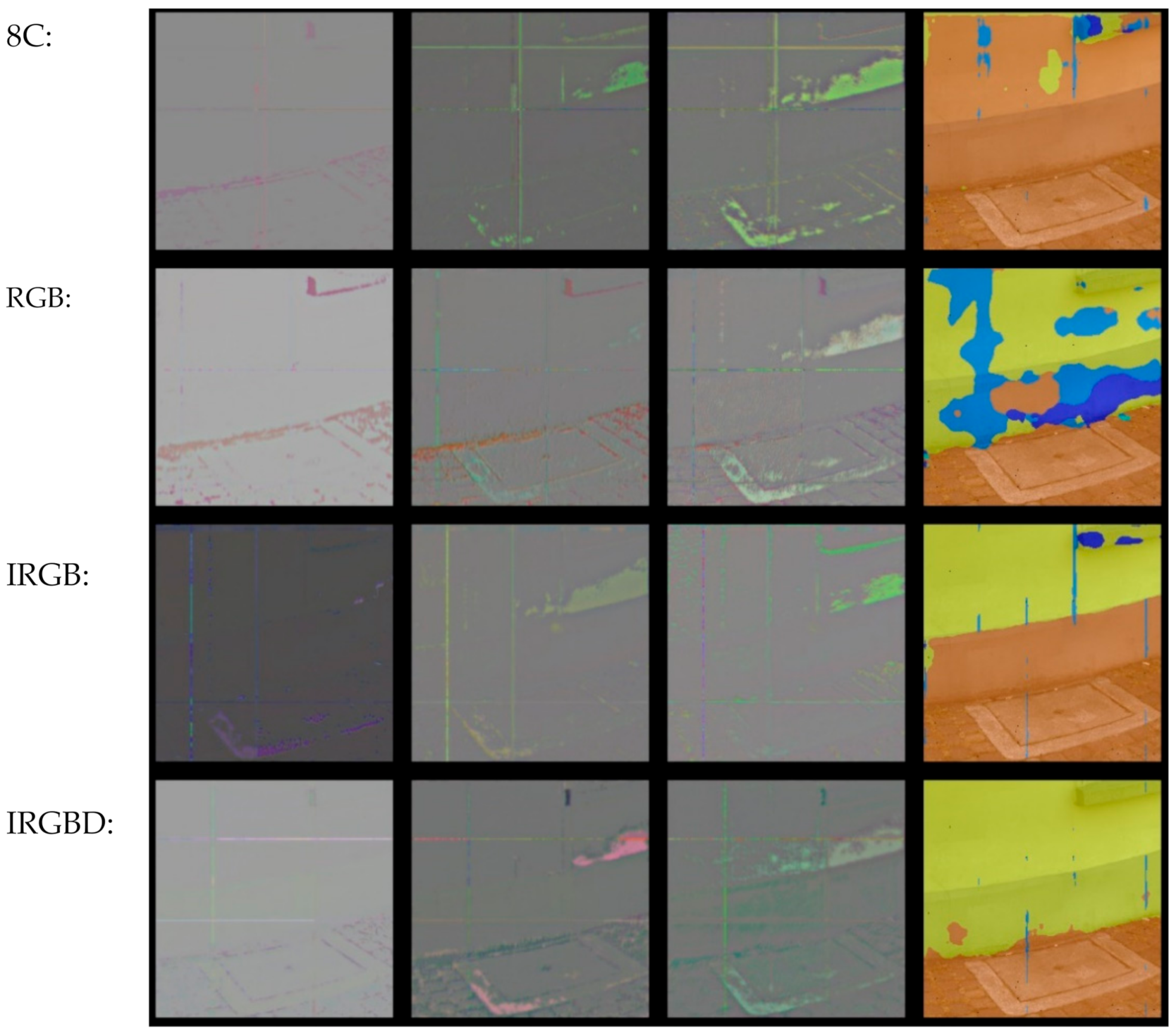
Moreover, it is noticed that the simple mixture of all the available channels (i.e., column 8C in Table 4 and Table 5) often results in a worse performance compared to that of combinations with fewer channels. To explore this thoroughly, for channel combinations 8C, RGB, IRGB, and IRGBD, the training curves for networks with the Inception-ResnetV2 backbone are plotted in Figure 5, and two test images are used to obtain the feature maps and corresponding segmentation results for comparison, as demonstrated in Figure 6 and Figure 7. From Figure 5, it is observed that the training process of combination of 8C converges much slower than others, which might indicate that the network struggled to learn the “correct” feature when there is a mixture of “useful” and “useless” data input. Taking the segmentation results in Figure 6 as an example, compared to the result of RGB combination, the additional I channel (i.e., IRGB) does help remove the mislabeled pixels in the wall region, but it also causes the mislabeling of the whole bottom part of the wall. The segmentation result is even worse for the 8C combination, which completely fails to distinguish the building and the road. A similar situation occurs for the street view test, as shown in Figure 7. Compared to the segmentation results for the RGB combination, the 8C combination causes a large mislabeling area around the road sign. Both test image results show that the IRGBD combination yields the best segmentation results.
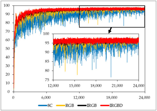
Figure 5.
Training accuracy for combinations of 8C (all the channels), RGB (color), IRGB (intensity and color), and IRGBD (intensity, color and depth) using networks of Inception-ResnetV2 backbone.

Figure 6.
Feature maps and segmentation results for four combinations for the building-road joint image.
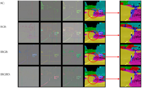
Figure 7.
Feature maps and segmentation results for four combinations in the street view image.
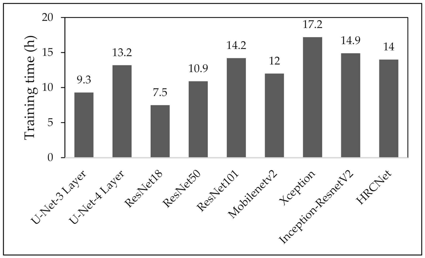
The average time of single training for nine networks are summarized in Figure 8, where the average time of Xception (17.2 h) is two times more than that of ResNet18 (7.5 h). Moreover, since the channel analysis requires a series of comparative tests to ascertain the optimal channel combination, the differences in training time between the networks are magnified. For example, the total channel analysis time for ResNet18 and Xception are 97.4 and 193.6 h, respectively. Since the previous investigation shows a high consistency of optimal channel combination across different networks, the efficiency can be improved significantly by conducting the channel analysis on a small network before training on more sophisticated networks. In addition, the total inference time (including PAN image generation, inference, back-projection) is around 170 k points/s.

Figure 8.
Summary of the average time of single training for nine network structures.
Finally, since the IRGBD channel combination and HRCNet got the best performance (mIoU is more critical than OA) in our previous testing, they were selected to evaluate the performance on the Semantic3D (reduced-8) test dataset. The reason to choose the reduced-8 rather than the high-density test dataset is that previous methods (especially point-based methods) are often tested on the reduced-8 test dataset as they cannot handle high-density point clouds efficiently. The complete training dataset (15 point clouds) was used in this stage, and the training protocol remains the same as mentioned in Section 2.3. The quantitative segmentation results are summarized in Table 8 below, where XJTLU outperforms previous best image-based methods by 4.4% regarding mIoU, and even outperforms several recently published point/discretization-based methods, which show the effectiveness of our proposed methods.

Table 8.
Quantitative results of different approaches on Semantic3D (reduced-8) [20]. Accessed on 16 March 2021 (the overperformed methods are marked in grey).
5. Conclusions
With the development of CIM, there is an increasing demand for high-precision semantic segmentation information. Data fusion is an emerging method to improve the segmentation performance. However, without a selection of effective data fusion sources, extra effort is required in both data collection and processing. Therefore, an efficient data fusion approach is proposed in this article by exploring the optimal combination of data channels. The analysis on the performance of different combinations of data channels is applied to obtain the optimal combination by adopting various neural networks. The robustness of the optimal combination is proved using a case study, which demonstrates the feasibility of the proposed data fusion channel selection. The findings can be utilized to achieve a significant improvement on efficiency by adopting a simple structured network for the channel analysis before applying a more complex network. In addition, the case study demonstrates that, without adopting this framework, a simple mixture of available data sources impairs the segmentation performance, which shows the necessity of channel selection in data fusion. Finally, using the selected channel combination and network, we achieved the best performance among image-based methods and outperformed several recent point/discretization-based methods.
Although the feasibility of the proposed method has been investigated on 2D convolutional neural networks, other types of networks exist that could be used for semantic segmentation in CIM, such as vision transformer [38] and point-based network [18]. Therefore, our future work will focus on the investigation of the robustness of the optimal combination of data sources among different types of networks.
Author Contributions
Conceptualization, C.Z.; formal analysis, Y.C.; funding acquisition, C.Z. and L.F.; investigation, K.W. and F.G.; methodology, Y.C., H.H., and C.Z.; supervision, C.Z.; writing—original draft, Y.C., Kaiyang Wang, and H.H.; writing—review and editing, C.Z., L.F., and F.G. All authors have read and agreed to the published version of the manuscript.
Funding
This research was funded by Xi’an Jiaotong-Liverpool University Key Program Special Fund (grant numbers KSF-E-04 and KSF-E-40) and Xi’an Jiaotong-Liverpool University Research Enhancement Fund (REF-17-01-11).
Institutional Review Board Statement
Not applicable.
Informed Consent Statement
Not applicable.
Data Availability Statement
The data presented in this study are openly available in [http://www.semantic3d.net/] at [arXiv:1704.03847], reference number [20].
Conflicts of Interest
The authors declare no conflict of interest.
References
- Stojanovski, T. City Information Modelling (CIM) and Urban Design. City Model. GIS 2018, 36, 506–516. [Google Scholar]
- Xu, X.; Ding, L.; Luo, H.; Ma, L. From Building iInformation Modeling to City Information Modeling. J. Inf. Technol. Construct. 2014, 19, 292–307. [Google Scholar]
- Lu, Q.; Lee, S. Image-Based Technologies for Constructing As-Is Building Information Models for Existing Buildings. J. Comput. Civ. Eng. 2017, 31, 04017005. [Google Scholar] [CrossRef]
- Golparvar-Fard, M.; Bohn, J.; Teizer, J.; Savarese, S.; Peña-Mora, F. Evaluation of image-based modeling and laser scanning accuracy for emerging automated performance monitoring techniques. Autom. Constr. 2011, 20, 1143–1155. [Google Scholar] [CrossRef]
- Kim, S.; Kim, S.; Lee, D.E. 3D Point Cloud and BIM-Based Reconstruction for Evaluation of Project by As-Planned and As-Built. Remote Sens. 2020, 12, 1457. [Google Scholar] [CrossRef]
- Badenko, V.; Fedotov, A.; Zotov, D.; Lytkin, S.; Volgin, D.; Garg, R.D.; Min, L. Scan-to-BIM Methodology Adapted for Different Application. Photogramm. Remote Sens. Spat. Inf. Sci. 2019, 42, 24–25. [Google Scholar] [CrossRef]
- Bernat, M.; Janowski, A.; Rzepa, S.; Sobieraj, A.; Szulwic, J. Studies on the use of terrestrial laser scanning in the maintenance of buildings belonging to the cultural heritage. In Proceedings of the 14th Geoconference on Informatics, Geoinformatics and Remote Sensing, SGEM, ORG, Albena, Bulgaria, 17–26 June 2014; pp. 307–318. [Google Scholar]
- Yang, R.; Su, L.; Zhao, X.; Wan, H.; Sun, J. Representative band selection for hyperspectral image classification. J. Vis. Commun. Image Represent 2017, 48, 396–403. [Google Scholar] [CrossRef]
- Li, Y.; Majumder, A.; Zhang, H.; Gopi, M. Optimized multi-spectral filter array based imaging of natural scenes. Sensors 2018, 18, 1172. [Google Scholar] [CrossRef] [PubMed]
- Abdalla, A.; Cen, H.; Abdel-Rahman, E.; Wan, L.; He, Y. Color Calibration of Proximal Sensing RGB Images of Oilseed Rape Canopy via Deep Learning Combined with K-Means Algorithm. Remote Sens. 2019, 11, 3001. [Google Scholar] [CrossRef]
- Bhuiyan, M.A.E.; Witharana, C.; Liljedahl, A.K.; Jones, B.M.; Daanen, R.; Epstein, H.E.; Kent, K.; Griffin, C.G.; Agnew, A. Understanding the Effects of Optimal Combination of Spectral Bands on Deep Learning Model Predictions: A Case Study Based on Permafrost Tundra Landform Mapping Using High Resolution Multispectral Satellite Imagery. J. Imaging 2020, 6, 97. [Google Scholar] [CrossRef]
- Park, J.H.; Inamori, T.; Hamaguchi, R.; Otsuki, K.; Kim, J.E.; Yamaoka, K. RGB Image Prioritization Using Convolutional Neural Network on a Microprocessor for Nanosatellites. Remote Sens. 2020, 12, 3941. [Google Scholar] [CrossRef]
- Pierdicca, R.; Paolanti, M.; Matrone, F.; Martini, M.; Morbidoni, C.; Malinverni, E.S.; Frontoni, E.; Lingua, A.M. Point cloud semantic segmentation using a deep learning framework for cultural heritage. Remote Sens. 2020, 12, 1005. [Google Scholar] [CrossRef]
- Alshawabkeh, Y. Linear feature extraction from point cloud using color information. Herit. Sci. 2020, 8, 28. [Google Scholar] [CrossRef]
- Meyer, G.P.; Charland, J.; Hegde, D.; Laddha, A.; Vallespi-Gonzalez, C. Sensor fusion for joint 3d object detection and semantic segmentation. In Proceedings of the IEEE/CVF Conference on Computer Vision and Pattern Recognition Workshops, Seattle, WA, USA, 14–19 June 2020. [Google Scholar]
- Lawin, F.J.; Danelljan, M.; Tosteberg, P.; Bhat, G.; Khan, F.S.; Felsberg, M. Proceedings of the Deep projective 3D semantic segmentation. International Conference on Computer Analysis of Images and Patterns, Ystad, Sweden, 22–24 August 2017; Springer: Cham, Switzerland, 2017; pp. 95–107. [Google Scholar]
- Guo, Y.; Wang, H.; Hu, Q.; Liu, H.; Liu, L.; Bennamoun, M. Deep learning for 3d point clouds: A survey. In IEEE Transactions on Pattern Analysis and Machine Intelligence; IEEE: New York, NY, USA, 2020. [Google Scholar]
- Hu, Q.; Yang, B.; Xie, L.; Rosa, S.; Markham, A. RandLA-Net: Efficient Semantic Segmentation of Large-Scale Point Clouds. In Proceedings of the 2020 IEEE/CVF Conference on Computer Vision and Pattern Recognition (CVPR), Seattle, WA, USA, 14–19 June 2020. [Google Scholar]
- Boulch, A.; Guerry, Y.; Le Saux, B.; Audebert, N. SnapNet: 3D point cloud semantic labeling with 2D deep segmentation networks. Comput. Graph. 2018, 71, 189–198. [Google Scholar] [CrossRef]
- Hackel, T.; Savinov, N.; Ladicky, L.; Wegner, J.D.; Schindler, K.; Pollefeys, M. Semantic3D.net: A new large-scale point cloud classification benchmark. arXiv 2017, arXiv:1704.03847. [Google Scholar] [CrossRef]
- Gull, S.F. Skilling. October. Maximum entropy method in image processing. In IEE Proceedings F Communications, Radar and Signal Processing; IET Digital Library: Guangzhou, China, 1984; Volume 131, pp. 646–659. [Google Scholar]
- Ronneberger, O.; Fischer, P.; Brox, T. U-net: Convolutional networks for biomedical image segmentation. In Proceedings of the International Conference on Medical Image Computing and Computer-Assisted Intervention, Munich, Germany, 5–9 October 2015; pp. 234–241. [Google Scholar]
- He, K.; Zhang, X.; Ren, S.; Sun, J. Deep residual learning for image recognition. In Proceedings of the IEEE Computer Society Conference on Computer Vision and Pattern Recognition, Las Vegas, NV, USA, 27–30 June 2016; pp. 770–778. [Google Scholar]
- Sandler, M.; Howard, A.; Zhu, M.; Zhmoginov, A.; Chen, L.C. Inverted Residuals and Linear Bottlenecks: Mobile Networks for Classification, Detection and Segmentation. In Proceedings of the IEEE Computer Society Conference on Computer Vision and Pattern Recognition, Salt Lake City, UT, USA, 18–22 June 2018; pp. 4510–4520. [Google Scholar]
- Chollet, F. Xception: Deep learning with depthwise separable convolutions. In Proceedings of the 30th IEEE Conference on Computer Vision and Pattern Recognition, CVPR 2017, Las Vegas, NV, USA, 27–30 June 2016; pp. 1800–1807. [Google Scholar]
- Hand, D.J. Data clustering: Theory, algorithms, and applications by guojun gan, chaoqun ma, jianhong wu. Int. Stat. Rev. 2010, 76, 141. [Google Scholar] [CrossRef]
- Szegedy, C.; Ioffe, S.; Vanhoucke, V.; Alemi, A.A. Inception-v4, inception-ResNet and the impact of residual connections on learning. In Proceedings of the 31st AAAI Conference on Artificial Intelligence, AAAI 2017, Francisco, CA, USA, 4–9 February 2017; pp. 4278–4284. [Google Scholar]
- Xu, Z.; Zhang, W.; Zhang, T.; Li, J. Hrcnet: High-resolution context extraction network for semantic segmentation of remote sensing images. Remote Sens. 2021, 13, 71. [Google Scholar] [CrossRef]
- Wang, J.; Sun, K.; Cheng, T.; Jiang, B.; Xiao, B. Deep High-Resolution Representation Learning for Visual Recognition. In IEEE Transactions on Pattern Analysis and Machine Intelligence; IEEE: New York, NY, USA, 2018. [Google Scholar]
- Zhao, H.; Shi, J.; Qi, X.; Wang, X.; Jia, J. Pyramid scene parsing network. In Proceedings of the 30th IEEE Conference on Computer Vision and Pattern Recognition, CVPR 2017, Honolulu, HI, USA, 21–26 July 2017; pp. 6230–6239. [Google Scholar]
- Zhao, H.; Zhang, Y.; Liu, S.; Shi, J.; Loy, C.C.; Lin, D.; Jia, J. Psanet: Point-wise spatial attention network for scene parsing. In Proceedings of the European Conference on Computer Vision (ECCV), Munich, Germany, 8–14 September 2018; pp. 267–283. [Google Scholar]
- Tchapmi, L.; Choy, C.; Armeni, I.; Gwak, J.; Savarese, S. SEGCloud: Semantic segmentation of 3D point clouds. In Proceedings of the 2017 International Conference on 3D Vision, 3DV 2017, Qingdao, China, 10–12 October 2017; Institute of Electrical and Electronics Engineers Inc.: New York, NY, USA, 2017; pp. 537–547. [Google Scholar] [CrossRef]
- Thomas, H.; Goulette, F.; Deschaud, J.E.; Marcotegui, B.; Gall, Y.L. Semantic classification of 3d point clouds with multiscale spherical neighborhoods. In Proceedings of the 2018 International Conference on 3D Vision, 3DV 2018, Verona, Italy, 5–8 September 2018; Institute of Electrical and Electronics Engineers Inc.: New York, NY, USA, 2018; pp. 390–398. [Google Scholar] [CrossRef]
- Contreras, J.; Denzler, J. Edge-Convolution Point Net for Semantic Segmentation of Large-Scale Point Clouds. In Proceedings of the International Geoscience and Remote Sensing Symposium (IGARSS), Yokohama, Japan, 28 July–2 August 2019; Institute of Electrical and Electronics Engineers Inc.: New York, NY, USA, 2019; pp. 5236–5239. [Google Scholar] [CrossRef]
- Zhang, Z.; Hua, B.S.; Yeung, S.K. ShellNet: Efficient point cloud convolutional neural networks using concentric shells statistics. In Proceedings of the IEEE International Conference on Computer Vision, Thessaloniki, Greece, 23–25 September 2019; Institute of Electrical and Electronics Engineers Inc.: New York, NY, USA, 2019; pp. 1607–1616. [Google Scholar] [CrossRef]
- Wang, F.; Zhuang, Y.; Gu, H.; Hu, H. OctreeNet: A Novel Sparse 3-D Convolutional Neural Network for Real-Time 3-D Outdoor Scene Analysis. IEEE Trans. Autom. Sci. Eng. 2020, 17, 735–747. [Google Scholar] [CrossRef]
- Wang, L.; Huang, Y.; Hou, Y.; Zhang, S.; Shan, J. Graph attention convolution for point cloud semantic segmentation. In Proceedings of the IEEE Computer Society Conference on Computer Vision and Pattern Recognition; IEEE Computer Society: Washington, DC, USA, 2019; pp. 10288–10297. [Google Scholar] [CrossRef]
- Wu, B.; Xu, C.; Dai, X.; Wan, A.; Zhang, P.; Tomizuka, M.; Keutzer, K.; Vajda, P. Visual transformers: Token-based image representation and processing for computer vision. arXiv 2020, arXiv:2006.03677. [Google Scholar]
Publisher’s Note: MDPI stays neutral with regard to jurisdictional claims in published maps and institutional affiliations. |
© 2021 by the authors. Licensee MDPI, Basel, Switzerland. This article is an open access article distributed under the terms and conditions of the Creative Commons Attribution (CC BY) license (https://creativecommons.org/licenses/by/4.0/).


