Abstract
Vibration monitoring is a frequent task within the general topic of Structural Health Monitoring. For this monitoring, usually accelerometers, strain gauges, fibre optic sensors or Global Navigation Satellite System (GNSS) receivers are placed on pre-selected positions on the structure and the point-wise measurements are individually processed to estimate the relevant modal parameters, for example, oscillating amplitudes and natural frequencies. If laser scanners were used for vibration monitoring, the analyses could be performed with a significantly higher spatial resolution that would be beneficial especially for locating structural weaknesses. However, to apply laser scanners rigorously to vibration monitoring, spatio-temporal models need to be set up. With this study, we develop and discuss four spatio-temporal models applied to the simulated vibration monitoring of a bridge deck. Therefore, we formulate either functional as well as stochastic connections between neighbored measurement positions within the estimation of the parameters of a harmonic oscillation. We reveal that those models allow an improved parameter estimation compared to the usually used strategies—even at lower measurement frequencies and shorter observation lengths.
Keywords:
harmonic oscillation; frequency; amplitude; Nyquist frequency; leakage effect; correlation 1. Introduction
In the context of Structural Health Monitoring (SHM), the vibration monitoring of civil infrastructure plays an important role [1]. Especially the vibration analysis of bridges using accelerometers [2,3,4,5], strain gauges [6], fibre optic sensors [7] or Global Navigation Satellite System (GNSS) receivers [8,9] is widespread in the field of SHM. Herein, several of these sensors are positioned on the structure to monitor its vibration. Within the operational modal analysis, usually natural frequencies, damping ratios and mode shapes are to be identified [10]. While these analyses, in the first place, are only performed individually for each measurement position, they are spatially interpolated in several applications in sense of a spatially continuous (operational) modal analysis of the complete construction [11]. This procedure only works out properly, if
- the observation length is long enough,
- the sampling rate of the sensors is high enough,
- the positions of the sensors are chosen properly.
Sampling rates that are too small would otherwise hinder the detection of high-frequency oscillations due to aliasing effects. The minimal sampling rate is determined by the Nyquist frequency [12]. Observation lengths that are too short would lead to a pronounced leakage effect hindering the sharp detection of relevant frequencies [12,13]. This latter effect is only relevant for short term (modal) analyses. Using only few sensors—leading to large distances between the sensor positions—would hide local abnormalities in the oscillation behavior of the structure. With this study, we highlight that these prerequisites can be softened in case that the measurements are analyzed not individually for each measurement position but combined in a spatio-temporal model.
In the field of geodesy, using a profile laser scanner for monitoring dynamic deformations of elongated structures as, for example, bridges, has become famous within the last years [14,15]. Profile laser scanners rapidly measure the surface of a structure with thousands of points having a point spacing of down to millimeters with a repetition rate of up to 200 Hz. While these are positive characteristics regarding the ability of using laser scanners for vibration analysis or SHM in general, their drawback is that the individual point positions on the structure cannot be determined a priori, that this point position is only limitedly stable between subsequent repetitions and that the object is measured point-after-point at each position.
These disadvantages have been met by the development of procedures transitioning from measured points to virtual reproducible points, for example, by means of spatially constant segments. However, since these procedures aggregate points of different positions to a single virtual point, both amplitude and phase get blurred. Consequently, other strategies for data mining within the measured times series are needed.
In this sense, we, in this study, derive spatio-temporal models in four steps beginning from the benchmark method of analyzing the vibration for each measurement position individually. Step by step we introduce further spatial connections between neighbored measurement positions to gain in the end a fully continuous spatio-temporal model for analyzing all measurements at different positions in combination. Doing so, the parameter identification process is improved due to a larger redundancy in the estimation process leading to smaller parameter uncertainties and higher reliability. Herein, we specifically aim at evaluating the benefit of each new spatial connection onto the parameter identification.
By this procedure, we focus on four main questions that are raised:
- 1.
- How can spatio-temporal models be formulated?
- 2.
- Can we reduce the observation length using these models maintaining the parameters’ uncertainty?
- 3.
- Can we reduce the sampling rate using these models maintaining the parameters’ uncertainty?
- 4.
- Do these models require a small spatial distance between the measured positions?
We relate the answers to the benchmark method that does not introduce any spatial connections between measurement positions at all during the parameter identification process.
These questions will be answered related to profile laser scanners due to the aforementioned properties. We additionally focus on elongated structures as bridges. Anyway, a transfer to other sensors and also other structures, even considering structures expanded in two dimensions, is also valid. In this first study, we only focus on an analysis in the time domain not considering transformations in the frequency domain, for example, based on a Fourier transformation [12] or wavelets [13].
Our analysis rests upon the simulation of a line oscillating with one single natural frequency being considered as a very simplistic realization of a bridge deck. The corresponding measurements of the laser scanner are simulated as well. We use simulations to clearly extract the benefit of the shown spatio-temporal models independent from other effects that would occur in empirical measurements. Although the simulation of a vibrating line might appear to be too simplistic, it clearly can serve as a first time analysis of the benefit when using spatio-temporal models for vibration analysis. The main conclusions of the results will be transferable to more complex scenarios that we will examine in future studies along with real world examples.
2. Relation to Vibration Monitoring
SHM can loosely be defined as the observation and interpretation of the performance of civil infrastructure as bridges, dams, towers, buildings, tunnels, docks and so forth. The aim is to assure the fitness of those structures, that is, a safe and economical operation. Therefore, a physical or parametric model of the structure is continuously identified using time-dependent data [1].
As one subdomain within SHM, vibration monitoring measures the vibration response of a structure—that is due to forced or ambient excitation—to identify modal characteristics, for example, natural frequencies, damping ratios and mode shapes, and their temporal changes. Temporal changes or local abnormalities in these modal characteristics—that is, changes of the natural frequencies, mode shape changes, mode shape curvature, flexibility and others [10,16]—indicate damages of the structures [17]. Those damages might be located and quantified by vibration monitoring. Thus, this modal analysis can reveal structural weaknesses, fatigue or deficiencies amplified or induced by unforeseen events [18].
The strategies of vibration monitoring can be separated into long term monitoring and short term monitoring. Short term vibration measurements are specially used to check key modal parameters used at the design stage and to verify the design. Short term measurements with high sensor density sometimes also provide a starting point for long term monitoring with a small set of instrumentation [19]. Since those short term measurement campaigns are not continuously ongoing, they only seek to identify the state of the structure at a specific time. They are sometimes only referred to as load tests or modal tests—distinguished from a (continuous) SHM [1].
The realization of a vibration monitoring bases upon the selection of an appropriate instrumentation or choice of sensors, respectively. Herein, accelerometers are quite famous [2,3,4,5] since they measure with a high sampling rate up to several kHz the second derivative of the displacement. Also frequently used for vibration monitoring are GNSS antennas and receivers (only for bridges) [8,9,20,21,22] or inclinometers [23,24,25]. With GNSS, the displacement is measured with a sampling rate up to about 10 Hz and with inclinometers, the derivative of the displacement with the position with up to kHz—depending on their measuring principle. In pilot tests, also robotic total stations or image-assisted total stations have been used [26,27]. These instruments measure—electro-optically or with an integrated camera via photogrammetry—the three dimensional position of a signalized target on a structure with sampling rates up to 10 Hz or higher.
All these sensors—or corresponding adapters—are fixed to the vibrating structure at certain positions that are pre-selected by the executing experts. The number of used sensors or adapters, respectively, depends on the size of the vibrating structure keeping economic aspects in mind. Choosing the number and position of sensors is of high relevance especially if the task of the vibration monitoring is not only (a) to determine that damage is present in the structure but also (b) to determine the geometric location of the damage, what is a frequent task [28]. The high relevance is governed by the fact that the measurements are processed individually for each measurement position. The estimated parameters of each position, for example, natural frequencies and damping ratios, are only afterwards spatially combined to gain the modal shapes.
Consequently, an inappropriate pre-selection of measurement positions hinders the SHM. In the worst case, potential damage might not be locatable or even detectable due to too low signal-to-noise ratios at the chosen positions. To compensate this situation, methods are needed to filter out environmental and noise effects [29,30] and also to deal with effects of measurement and modelling uncertainties [1]. Alternatively, spatio-temporal models could be developed connecting neighbored sensor measurements as is focused within this study.
Another group of sensors is able to measure vibrations without the need for previous installation on the structure, that is, they enable contact-less measurements: terrestrial laser scanners and vibrometers. Terrestrial laser scanners measure the environment in three dimensions by a rotating mirror that deflects a laser beam whose time-of-flight is measured to the structure [31]. In general, terrestrial laser scanners have shown their great potential for monitoring the displacement or deformation, respectively, of structures based on a variety of corresponding publications: damage detection of bridges [32,33,34], metal beams [35] water dams [36], radio telescopes [37] and historic or other buildings [38,39,40]. Neuner et al. (2016) [41] give a further overview. In all these studies, the structure is assumed to remain static during the data acquisition that usually takes from some seconds to several hours. Thus, laser scanners are rather used to monitor geometric long-term changes via surface movement over time [42,43].
For measuring the geometry of elongated structures, scanning a two-dimensional profile along the structure’s main extent might be sufficient. For this task, profile laser scanners might be used—they measure the surrounding only in two dimensions with a sampling rate of up to 200 Hz at a point spacing on the structure up to some millimeters in 10 m distance. Thus, they could also be used for monitoring short-term changes as vibrations [15,44].
Vibrometers measure distance changes to the structure in the line-of-sight of the optical sensor axis using interferometry with a sampling rate up to several MHz [45]. Vibrometers can also be enhanced with a comparable scanning mode leading to a continuous laser scanner doppler vibrometer measuring distance changes in rotating line-of-sights [45,46]. Instead of laser scanners, vibrometers are explicitly designed for monitoring dynamic displacements as shown, for example, in [47,48,49].
In all cases, utilizing the aforementioned contact-less sensors, one measures both spatial and temporal information about the structure, greatly reducing the testing time required for modal analysis. However, two aspects have to be noticed: Firstly, the measurement position on the structure cannot be pre-selected, it is a consequence of the chosen angular grid of measurements instead. Secondly, the structure is measured along its extent point-after-point, not simultaneously. Thus, the time needed for capturing the structure at all positions only once equals the measurement time for each measurement point multiplied with the number of points on the structure. This one-time capturing of the complete structure is named herewith one measurement epoch.
This non-simultaneous measurement of the structure at not selectable positions further strengthens the need of including spatio-temporal models into the data processing to connect the measurements with each other. Otherwise, spatial variations of the structure are not separable from temporal vibrations. This especially holds if the sampling rate is rather low compared to the oscillation frequency. Strategies to deal with these facts exist for vibrometers, for example, the demodulation method, where the velocity response of the interferometer is multiplied by sinusoidal signals at the excitation frequency and a low-pass filter is applied to obtain the deflection shape of the structure [46,50]. Thus, for this strategy, the excitation frequency needs to be known so that this method is rather applicable at forced excitation, for example, within fatigue checks.
For profile laser scanners, ref. [44] developed and [15] adapted a method to divide the measured structure into several segments in which all measurements are averaged. This strategy minimizes the noise in the measurements and it introduces a regular, equally-spaced grid. Within this grid, each measurement position is again processed individually and only afterwards combined in a spatial waterfall diagram. Thus, since no intra-epochal relations between measurement positions are formulated within this strategy, it only works for high sampling rates of the laser scanner related to the oscillation frequency of the structure: Only then, the structure might be considered as static within one measurement epoch.
Consequently, the latter sensors that densely measure spatial and temporal information, that is, vibrometers or laser scanners, require a spatio-temporal modelling for vibration monitoring. These models can be seen in the context of data mining of time series that is a relatively new aspect in vibration monitoring. Herein, the data is rather studied to reveal patterns, trends, relationships and anomalies [1]. For instance, [51] propose an automated modal identification procedure based on stochastic subspace identification and [52] identify natural frequencies of a bridge using Bayesian estimates and a reliability-based method.
Examples of these spatio-temporal models will be developed in the following section. Based on simulations, we will imply that these models further increase the usability of terrestrial laser scanners for vibration monitoring. This holds since the dense information in space and time improves the ability to determine the geometric location of a structure’s potential damage in sense of Level 2 within the system of classification for damage-identification methods [28].
3. Implementing a Simulation Environment
The implemented simulation environment rests upon an oscillating elongated structure, that is, a bridge deck, and a profile laser scanner digitizing this structure. The basics of profile laser scanners, the simulation, its parameters and the corresponding final measurements that are used as input for the spatio-temporal models are explained in the following.
3.1. Profile Laser Scanners
Profile laser scanners sample the environment within a two-dimensional profile leading to measured points with coordinates . They consist of a rotating mirror that deflects a laser beam where the rotation axis is orthogonal to the two-dimensional profile. The original observations of a profile laser scanner are the zenith angle, that is, the direction in which the mirror deflects the laser beam, as well as the distance between the scanner’s reference point and the structure that reflects the laser beam. The latter one is gained electro-optically via time-of-flight principle or amplitude-modulated-continuous-wave principle [31]. The structure itself does not need to be signalized or entered in any way for these measurements.
With the high-end laser scanner Profiler 9012 by Zoller+Fröhlich, a maximal rotation frequency of 200 Hz can be selected leading to 5120 points per 360 deg [53] or a point spacing of about 12 mm in 10 m distance, respectively. With lower rotation frequencies, smaller point spacings can be achieved. At distances of 10 m, the measured points’ accuracy is in the range of about 1 mm or better [54] if systematic errors are handled properly. Anyway, for the subsequent simulation, these characteristics are downgraded to show the potential of spatio-temporal models even for weaker laser scanner performances.
3.2. Basic Set-Up
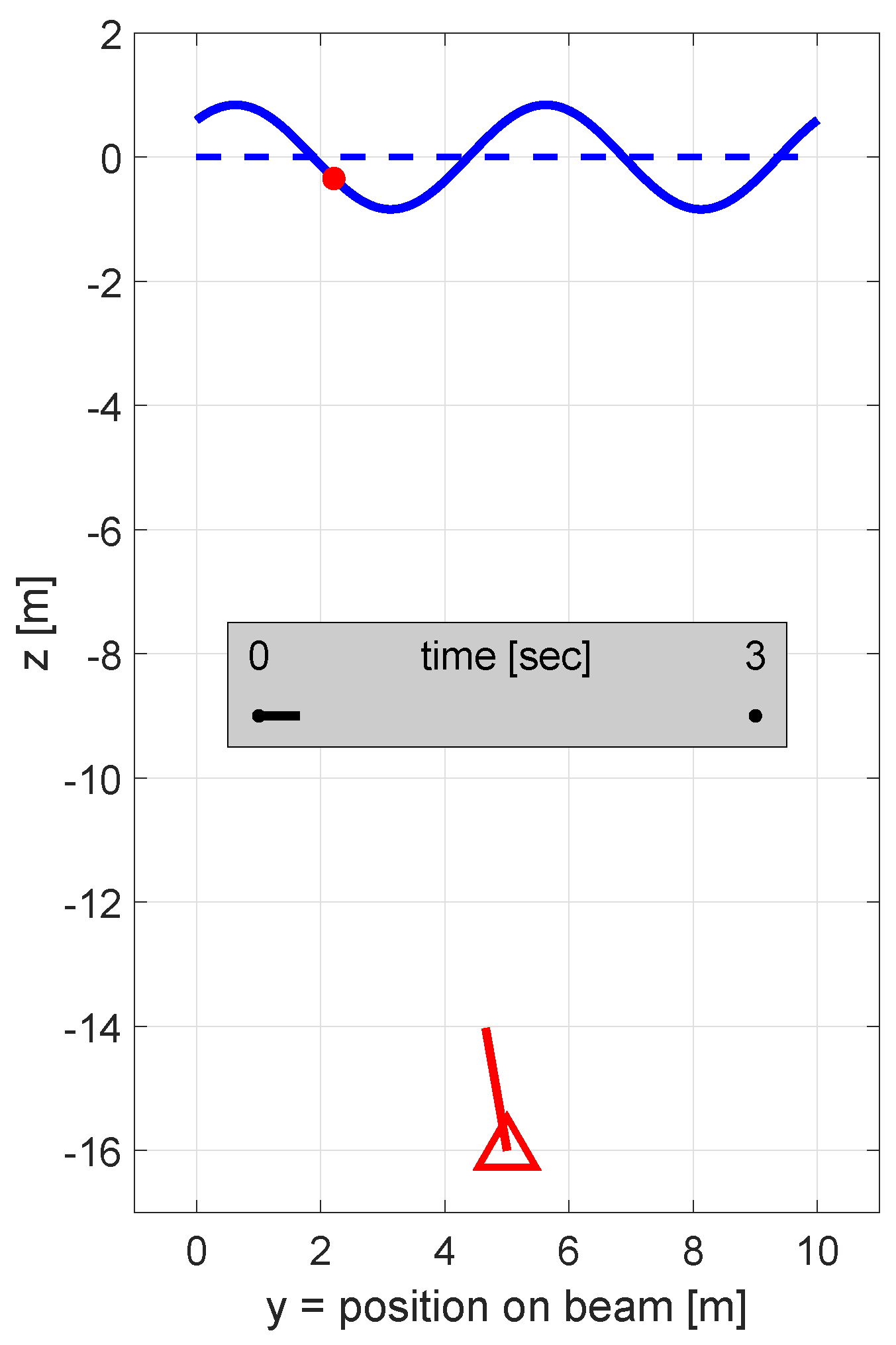
The simulation’s basic set-up is shown in Figure 1. It consists of a profile laser scanner whose distance measurement’s origin is positioned m centered under a structure that is extended in direction of the y-axis. This structure has a length of 10 m, its static state equals a simple horizontal line with . The structure is harmonically oscillating with a frequency of Hz, a maximal amplitude of mm and a phase of rad. The maximal amplitude itself is overlayed with a spatial oscillation to simulate that the structure deforms spatially. The frequency of this spatial oscillation equals m−1 leading to two complete wave cycles along the structure’s length of 10 m as shown in Figure 1.
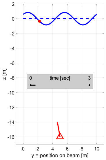
Figure 1.
Basic simulation with laser scanner (red triangle), direction of laser beam (solid red line), scan point on structure (red dot), static mean value of observed structure (dashed blue line) and oscillating structure (solid blue line, 20-times oversubscribed for better visibility).
Thus, we assume that the structure is supported by four plain bearings as the endpoints are not fixed, but allowed to move also. Furthermore, we only model one single natural frequency leading to only one mode shape. These assumption are rather simplistic but they are a starting point to evaluate the spatio-temporal models. In the future, we will also introduce further natural frequencies to also simulate and analyze the ability to identify the parameters of more complex systems and their impact on resulting mode shapes.
The profile laser scanner digitizes the oscillation of the structure with a frequency of 4 Hz for a duration of 3 s leading to 11 measured profiles or 11 epochs, respectively. The angular step-width equals 0.1 deg leading to 347 points on the structure with an approximate point spacing of 29 mm. For simplification, each point is noised in z-direction with mm while the y-direction is considered as error-free.
It has to be emphasized that the position of each point on the structure, that is, its y-coordinate, varies for each profile. This is due to (a) angular measurement noise of the profile laser scanner and (b) the fact that the point of intersection between oscillating structure and the direction of the laser beam depends on the current state of the structure, that is, the current extent of the oscillation at this position. This fact can only be considered rigorously by a spatio-temporal modelling as we intend to develop in this study.
The rather low frequency, the short observation length and the high noise are chosen in this basic set-up on purpose to highlight the benefit of the spatio-temporal models in Section 5 especially at challenging set-ups. By also introducing further set-ups (longer observation time, higher measurement frequency, smaller point spacing), we will evaluate the performance of spatio-temporal models with other foci, too.
Especially the needed observation length is of relevance here: It indicates how long the here presented data mining strategy needs to identify the current modal parameters. In sense of temporal changes in the modal parameters, eventually occurring within an ambient vibration monitoring, a reducible observation length increases the ability to detect temporal changes in these parameters due to changing excitations.
3.3. Resulting Measurements
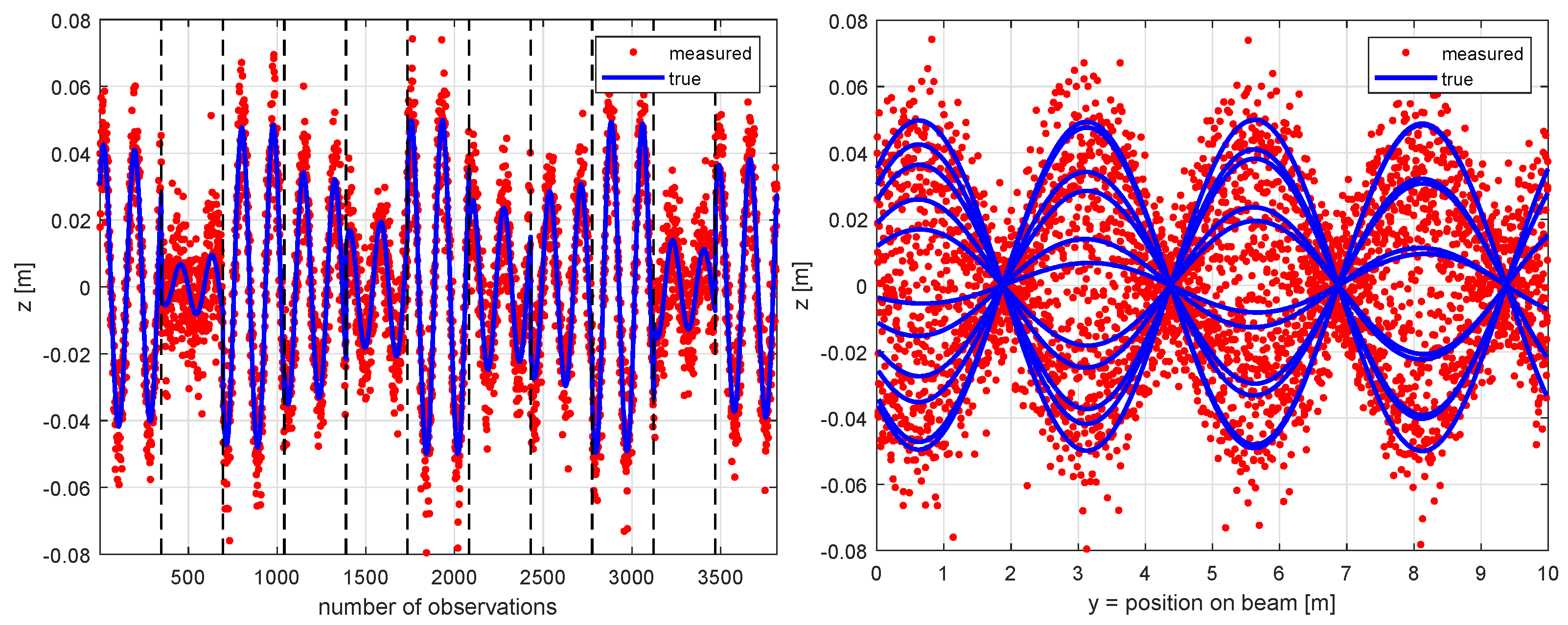
Based on the basic set-up introduced in the previous subsection, a times series containing 11 profiles with points each evolves. The total number of measurements equals, thus, . The true measurements are noised with the standard deviation of mm. This times series is depicted in Figure 2 left along the number of all measured points and Figure 2 right along the length of the measured beam. Figure 2 also shows the true oscillation differing from the observations due to the discrete sampling frequency of 4 Hz and the noise of 10 mm.
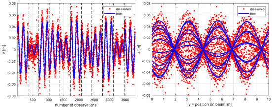
Figure 2.
Measured points (red dots), simulated oscillation (blue lines) in basic set-up along the number of measurements (left, vertical black dashed lines indicate new profile) and along the position on the beam (right).
Figure 2 implies two things: First, the laser scanner measures the oscillating structures in different states (see Figure 2 left). During some profiles (e.g., 3rd, 6th, 9th), the oscillation magnitude is nearly maximal and during other profiles (e.g., 2nd, 10th), it is minimal. If only looking at the noised measurements, an oscillation is hardly noticeable in the latter case.
Second, at some positions on the structure (i.e., m, m, m, m), the structure hardly oscillates at all (see Figure 2 right). This is due to the modelled spatial harmonic oscillation. As will be shown in the next section, the vibration analysis is challenging especially at these positions without proper spatio-temporal models. This holds for using profile laser scanners as well as for using accelerometers or GNSS receivers.
3.4. Vibration Analysis
We perform the vibration analysis by estimating the parameters of a temporal harmonic oscillation (mean value, amplitude, frequency, phase) based on the given measurements. The fact that the oscillation parameters might vary with the position on the structure is dealt with differently in the four steps of spatio-temporal modelling. In usual applications, this fact would just not be considered since the temporal harmonic oscillation is analyzed for each point individually as stated in Section 2.
The estimation is realized in a least-squares adjustment of parameters minimizing the square root or errors between measurements and estimated parameters [55,56]. The parameters that are to be estimated are formulated by the corresponding spatio-temporal model of each step that will be introduced in Equations (1)–(7). Herein, the parameters and the number of parameters differ between the steps leading to different results.
Since the adjustment will be non-linear in each case, approximate values are needed. These are gained by noising the true parameters defined in the simulation environment using the standard deviations of 0.10 m for the mean value and the amplitude, 0.05 Hz for the frequency and 0.10 rad for the phase. Investigations towards the sensitivity of the analysis regarding the approximate values will follow. As stochastic model, the true standard deviation of the measurements is included: mm.
4. Developing Spatio-Temporal Models
We develop the concept of a spatio-temporal vibration analysis based on four steps. In Step 1, we use the classical model of analyzing each measured position independent from the spatially neighbored points. Each further step introduces a connection between neighbored points to gain a fully continuous spatio-temporal model in the end.
4.1. Step 1
The first step equals the classical approach of parameterizing the temporal measurements z dependent on the time t at each position independent from the neighborhood:
Herein, the vibration is parameterized based on a harmonic oscillation using a mean value , an amplitude , a frequency and a phase . By the index i, we denote that the corresponding parameters are discrete in space. Hence, it is not a continuous consideration as will be introduced in step 4. For each of the 347 points on the structure, one set of oscillation parameters () is estimated according to Section 3.4 based on 11 measurements each, 3817 measurements in total.
An alternative formulation of this usual processing of step 1 is given by [15]. They average the points measured by a profile laser scanner in certain segments to cope with the fact that the individual point positions may change between different profiles and to reduce the noise in the measurements. Afterwards, they process the averaged points analogous to step 1 independent from the neighbored points without any spatio-temporal model. Thus, regarding the functional formulation, this procedure is similar to step 1 and Equation (1). We will discuss this strategy also briefly as step 1b in the following using a segment length of 0.25 m.
4.2. Step 2
Step 2 assumes that the oscillation frequency and the phase do not vary on the whole structure:
These assumptions are fulfilled within the current simulation; they are also meaningful for a real vibration monitoring: The oscillation frequency, that is, natural frequency, will most probably not change along the object, at least not between each measurement position. The phase describes the rest-part of the period that is identical for all points of the bridge deck, provided that the scanner rotates with a constant speed.
With these assumptions, the spatio-temporal model of step 1, Equation (1), simplifies to
meaning that only one single frequency f and phase are estimated according to Section 3.4 for the complete data set. Thus, the number of estimated parameters is reduced compared to step 1.
4.3. Step 3
Step 3 is a further advancement of step 2 that firstly considers all parameters () to be spatially connected. For the amplitude and the mean value, soft local constraints are integrated:
Hence, we allow the mean value and the amplitude to change only smoothly along the structure. This assumption is valid considering the fact that we deal with a continuous line in the simulation. The translation into real world examples is also feasible as bridges—at least partially—consist of continuous beams. At discontinuous positions, that is, at the transition of individual construction elements, especially the soft constraint concerning the smooth mean value would need to be softened more. However, the basic idea of a soft constraint is transferable in any case to real world examples as we generally monitor rather solid structures within a vibration analysis.
These soft constraints are realized by integrating stochastic pseudo-observations into the parameter identification according to Section 3.4. By this, we formulate constraints in the parameter estimation that should not be fulfilled strictly but with a rigorousness applied to the corresponding standard deviation [55,56]. This approach of modelling spatial connections between neighbored points equals, thus, a Markov process. Since two pseudo-observations can be introduced for each couple of neighbored points, the amount of observations increases compared to step 2.
The corresponding standard deviation of the pseudo-observations regulates the strictness of these soft conditions. We here assume the equality of neighbored mean values to be rather high leading to mm. Since the amplitudes indeed change over the length of the structure (see Figure 2 right), we set this standard deviation larger leading to mm.
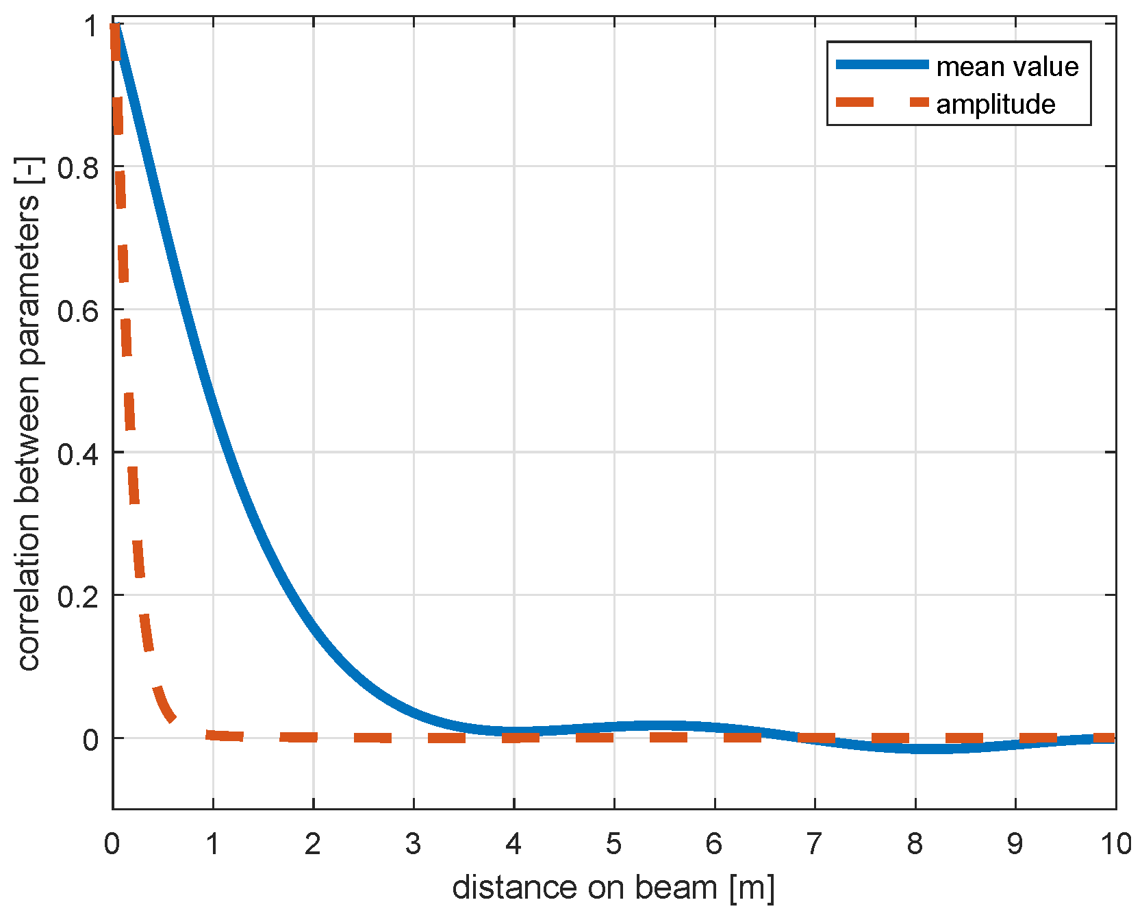
This approach using pseudo-observations in step 3 stochastically introduces spatio-temporal connections between the measured points and their oscillations. The resulting spatial connection between the measured points and the parameters can be highlighted by depicting the spatial correlation between the estimated mean values as well as between the estimated amplitudes , both along the distance between points on the beam (Figure 3): The estimated mean values mutually support each other (minimal correlation of 0.2) up to a point distance of about 1.8 m, the estimated amplitudes mutually support each other up to a point distance of about 0.3 m. Hence, each estimated mean value incorporates the information of about 60 neighbored points and each estimated amplitude the information of about 10 neighbored points, both considering point spacings of about 29 mm.
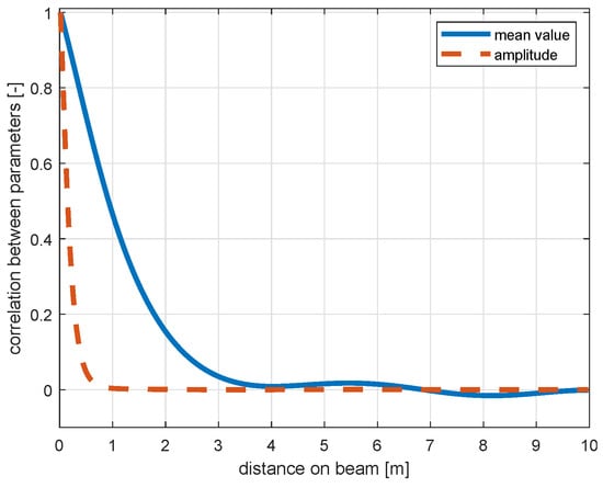
Figure 3.
Correlation between estimated mean values and between estimated amplitudes at step 3.
4.4. Step 4
In step 4, we finally introduce a continuous spatio-temporal model for the vibration analysis that does not anymore consider the observations and parameters at discrete positions but continuously in space . Therefore, we parameterize the measurements temporally and also spatially with the functional model of a harmonic oscillation:
Herein, we substitute the mean value continuously by the two parameters and of a linear trend. The amplitude is substituted by a spatial harmonic oscillation defined by the parameters . At all previous steps, the mean values and amplitude were estimated individually for each position. Thus, in step 4, the number of estimated parameters is reduced to seven: . Again, the parameter identification process is based on a least-squares estimation according to Section 3.4.
4.5. Impact of Spatio-Temporal Models on Reliability of Vibration Analysis
To further distinguish the different steps, we compare several quality measures: The redundancy, the relative redundancy and the partial redundancies. These values are measures to describe the reliability of an adjustment, that is, its ability to estimate unbiased parameters [56]. Herein, the focus can be lead on the contribution of all measurements, or individual ones, on the estimated parameters. In the field of geodesy, reliability measures are used quite frequently to extend the significance of the quality assessment of a parameter estimation that is otherwise only focused on accuracy and not on controllability as well [57].
Firstly, redundancies describe the absolute degrees of freedom of a complete adjustment. Secondly, relative redundancies quantify the relation between the redundancy and the number of measurements. Thirdly, partial redundancies split the complete redundancy down to each individual measurement. They explain for each measurement how much it is controlled by the others. If this control is high (high partial redundancies) and similar for all measurements, all measurements mutually support each other so that the parameters of the adjustment can be expected to be estimated unbiasedly with high precision. Relative redundancies and partial redundancies reach values between 0 and 1 for uncorrelated measurements as is the case in the present study [56].
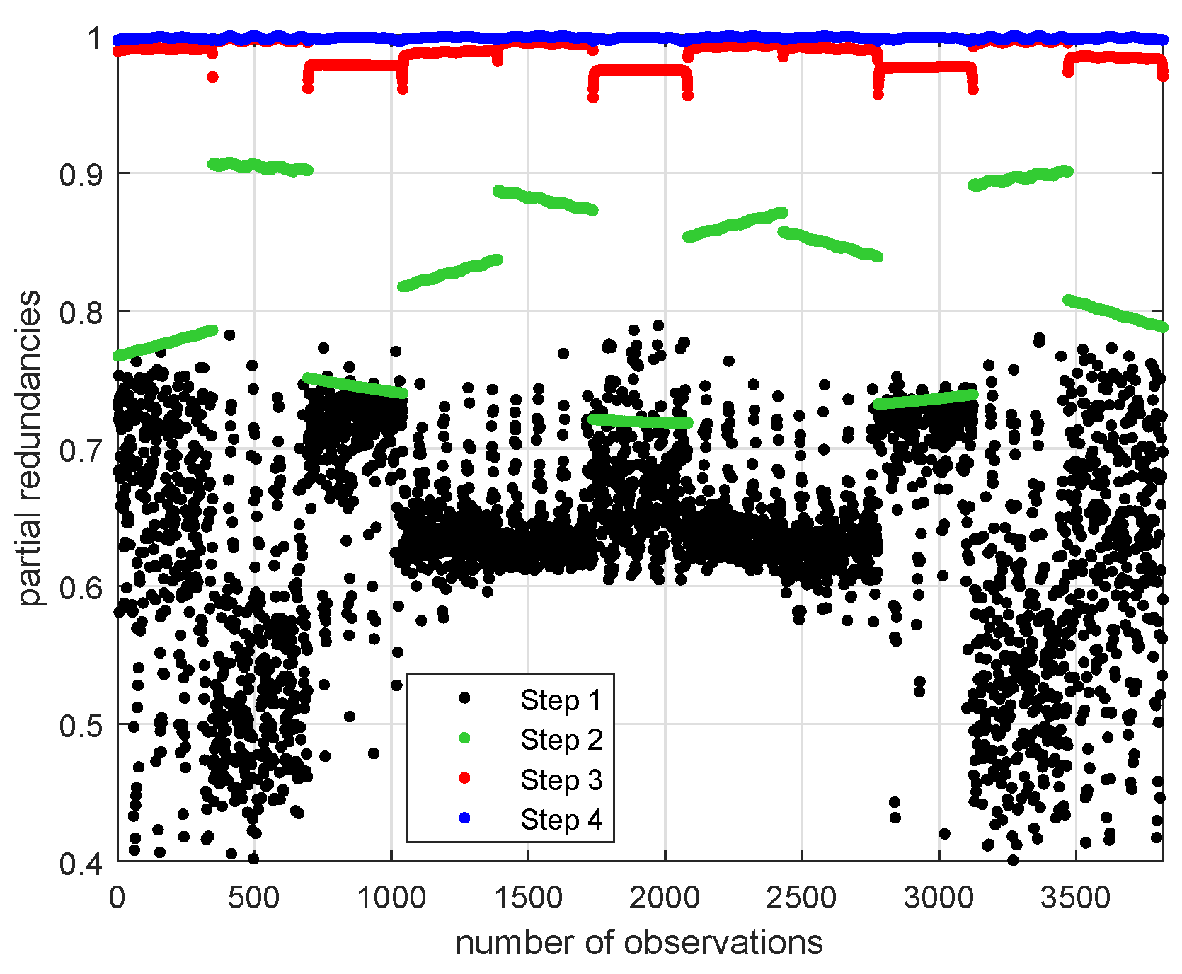
Table 1 and Figure 4 show the results for all steps. Table 1 implies that the redundancy becomes higher from step 1 to step 3—for step 4 it is slightly smaller than for step 3 due to the large number of pseudo-observations in step 3. Anyway, the relative redundancy reaches its maximum at step 4, while it is smaller at the other steps. Clearly, each step improves the situation compared to the usual step 1.

Table 1.
Number of measurements, number of parameters to be estimated, redundancy and relative redundancy for each step.
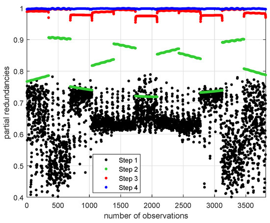
Figure 4.
Results of basic set-up: Partial redundancies.
Analyzing the partial redundancies in Figure 4, several effects are visible:
- With each new step, the variation in partial redundancies becomes smaller.
- With each new step, the partial redundancies increase.
- Assuming that the frequency and the phase of the oscillation are equal for all measured points (as we assume in steps 2, 3, 4), forces the partial redundancies of individual profiles to become more similar. This can be seen by the fact that in step 2 and 3, we can clearly distinguish the 11 profile measurements from each other.
- At step 2, it is visible that measurements of profiles with a nearly maximal oscillation magnitude (e.g., 3rd, 6th, 9th, see Figure 2 left), are not that controlled by the others, that is, the corresponding observations have rather low partial redundancies. Hence, these measurements are important to estimate the parameters with a high quality. On the contrary, profiles with a small oscillation magnitude (e.g., 2nd, 10th) have high partial redundancies meaning that they are not that important for the vibration analysis. This makes sense as, in that latter case, all observations describe a quite similar behavior regardless the position on the bridge.
- This effect also exists for step 3, but less pronounced.
- For the stochastic modelling in step 3, measurements at the begin and end of each profile are less controlled since the number of neighboring points is less towards the border.
- At step 4, there are barely any differences in the partial redundancies. This means that the continuous spatio-temporal modelling of this step indeed successfully incorporates all measurements quite similarly into the adjustment. Thus, profile measurements are important for this adjustment even if the oscillation magnitude is not high during the time of measurement (e.g., 2nd, 10th profile). At the same time, it is rarely important anymore at which position on the structure the measurement is performed—as was the case for step 2 and also with less emphasis for step 3. Thus, step 4 establishes an equilibrium of all measurements.
This analysis of the partial redundancies implies: When incorporating spatio-temporal models into the vibration analysis, the results are less sensitive to the individual measurement positions. The additional information in the analysis—included by functional or stochastic relations, improves the reliability and also the accuracy of the vibration analysis. Thus, to be more general—Strategies for data mining improve the vibration analysis.
5. Evaluating Spatio-Temporal Models
The evaluation complies with the questions asked in Section 1. Hence, we firstly analyze the basic set-up introduced in Section 3, afterwards we introduce further set-ups evaluating the spatio-temporal models regarding the observation length (set-up “length”), sampling rate (set-up “sampling rate”) and the spatial distance between measured points (set-up “point distance”). The corresponding changes compared to the basic set-up are given in Table 2. In all cases, we will evaluate and later on discuss the differences in the general behavior of each modelling step in the various set-ups. We will not evaluate the estimated quantities explicitly in detail since these are due to the specific conditions of the present simulation and not transferable.

Table 2.
Parameters of simulated set-ups.
In the analyses, we focus on the estimated amplitudes and frequencies since these are the most relevant values for a vibration analysis. The statements regarding the amplitudes are quite similar for the estimated mean values, the statements regarding the frequencies are quite similar for the estimated phases. Thus, they do not need to be explicitly shown and discussed.
5.1. Basic Set-Up
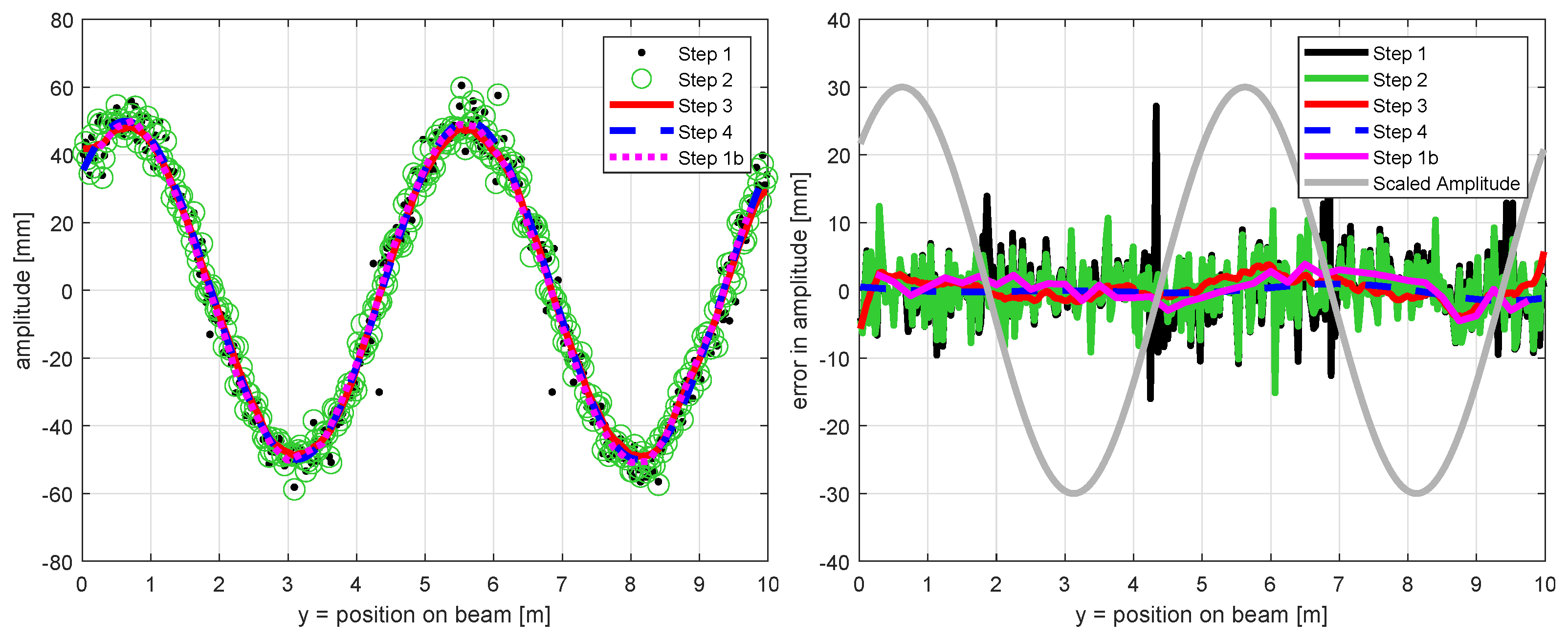
The estimated amplitudes and the errors in amplitudes, that is, the deviations from the true value, are depicted for the basic set-up in Figure 5. Figure 5 left shows that the general trend of the amplitudes can be estimated in all steps. The largest deviations from this trend (true amplitude of 50 mm) are archived for steps 1 and 2.
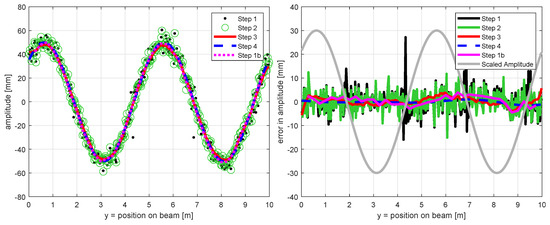
Figure 5.
Results of basic set-up: estimated amplitudes (left), errors in amplitude (right).
More details can be seen in Figure 5 right. The errors in steps 1b, 3 and 4 are remarkably smaller than for steps 1 and 2. For reasons of clarity, we also depicted in Figure 5 right the true scaled amplitude of the oscillation along the beam. Hence, for step 1, it is directly visible that the highest errors occur at the positions on the beam that oscillate the least (amplitude approximately zero). This can be expected: The amplitude is not predictable well if its value is low, that is, the signal-to-noise ratio is low. Contrary, the magnitude of the amplitude seems not to have an impact on the error for steps 2, 3 and 4 due to the modelled spatial connections.
For step 1b, the amplitude seem not to have an impact on the error, too. This is due to the fact that the segment length for averaging is chosen as 0.25 m leading to 8 or 9 points per segment (29 mm point distance). With a shorter segment length, the errors in amplitude would be higher (similar to steps 1 and 2). With a longer segment length, the errors would be smaller but with a larger systematic part due to the fact that the amplitude is assumed to be equal within this segment length.
The errors in amplitude are generally the smallest with step 4. Compared to step 4, step 3 and step 1b have larger errors with approximately equal magnitudes and similar trends.
Figure 6 depicts the errors in frequency where the true value of Hz has already been subtracted Clearly, step 1 leads to large errors in the estimated frequency. At positions on the beam with a small oscillation amplitude, the errors are up to an absolute value of many Hz or even kHz—again due to a low signal-to-noise ratio. Step 1b in fact decreases these errors, but it is still affected significantly by the signal-to-noise ratio of the oscillations since no spatial connection between all measurement positions is included. In this case, simply averaging neighboring measurements has only a limited effect on the accuracy of the frequency estimation. Consequently, we do not consider step 1b in the following evaluations any more.
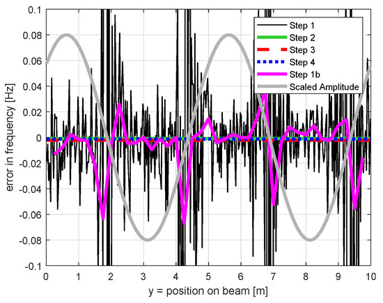
Figure 6.
Results of basic set-up: errors in frequency. For reasons of clarity, the vertical axis is limited to errors with an absolute magnitude of 0.1 Hz although values increase up to several kHz.
For steps 2, 3 and 4, only one single frequency is estimated, see Equations (4) and (7). In Figure 6, this single value is anyway depicted along the structure’s beam for better comparison with steps 1 and 1b. Herein, the estimated frequencies between steps 2, 3 and 4 are visually not distinguishable. Their differences are in the range of some mHz. Thus, all these steps remarkably improve the estimation of the frequency. The similarity in the results is due to the fact that all these steps model the frequency identically, that is, with one value not varying along the structure.
These previous numerical results are all based on one single simulation run whose observations are shown in Figure 2. However, we analyzed several simulation runs and attested the present one to be representative for the underlying stochastic process. We did not perform a Monte Carlo simulation for this basic set-up or the subsequent ones since our aim is not to provide generally valid numerical values for each spatio-temporal model. Rather, we want to point out structural benefits if using spatio-temporal models for vibration analysis of elongated structures.
5.2. Variation of Observation Length
Within this subsection, we analyze the effect of varying observation lengths on the estimated parameters. Therefore, we start with an observation length of 0.5 s and increase the length up to 20 s leading to a number of measured profiles (repetitions of measured points, that is, measurement epochs) ranging between 1 and 50 (Table 2). The sampling rate and the point spacing on the beam do not change here. We compare the results of the different set-ups along the variation of the observation length based on the standard deviations of the amplitudes and the frequencies:
- Amplitude
- In the steps 1, 2 and 3, we estimate one single amplitude for each repeatedly measured position on the structure. In step 4, we instead formulate a functional relation between all these amplitudes along the position of the structure (Equation (7)). Based on this functional relation, one single amplitude for each repeatedly measured position can be calculated again, analogous to steps 1, 2 and 3.
- Finally, we estimate the standard deviation of the errors of these amplitudes (Figure 7 left) to give only one single comparable number for the quality of the estimated amplitude for each observation length. Herein, we empirically build the standard deviation without accounting for possible correlations between the amplitudes.
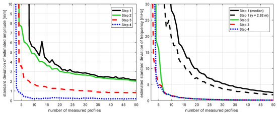 Figure 7. Results of set-up “length”: standard deviation of amplitude (left) and frequency (right). For reasons of clarity, the vertical axes are limited to 10 mm or 30 mHz, respectively, although larger values exist.
 - Thus, the values at a number of 11 measured profiles resemble the standard deviations of the errors in amplitude of the basic set-up shown in Figure 5 right.
- Frequency
- In step 1, we estimate one individual frequency for each repeatedly measured position on the beam (Equation (1)) and we also estimate the corresponding standard deviations. To get one single value for the complete simulation run, we build the median of these estimates (robust average of all values). Figure 7 right depicts the median of the estimated standard deviations of the frequencies for step 1.
- Additionally, we plot the estimated standard deviation for the position of m on the beam. At this position, the estimation is the best for step 1.
In general, Figure 7 left implies that increasing the observation length decreases the standard deviation of the estimated amplitudes and frequencies for all steps. However, significant differences are visible:
- Each step reduces the uncertainty compared to the previous ones.
- For steps 1 and 2, the uncertainty decreases with each additionally measured profile.
- For steps 3 and 4, the decrease is faster: About 20 or about 10 profiles, respectively, are already enough to get the smallest uncertainty. Afterwards, it does not decrease noticeably anymore with more profiles.
- The standard deviation of steps 1 and 2 is similar when measuring 50 profiles (or 20 s), the one of step 3 is about 50% smaller, the one of step 4 is about 85% smaller.
- Due to the fast decrease in uncertainty for steps 3 and 4, the benefit of those two steps compared to steps 1 and 2 further increases for shorter observation lengths.
Considering the results of the estimated frequencies (Figure 7 right), it is visible that all three steps that include spatial connections between the oscillations measured at the individual points improve the estimation noticeably. Starting from seven profiles, no differences are visible any more. This fits to Figure 6 (basic set-up with 11 measured profiles) where also no difference was visible. Compared to the best estimation of step 1 at the position m, the standard deviations of steps 2, 3 and 4 are about 95% smaller when measuring 20 s or 50 profiles, respectively.
5.3. Variation of Sampling Rate of Measurements
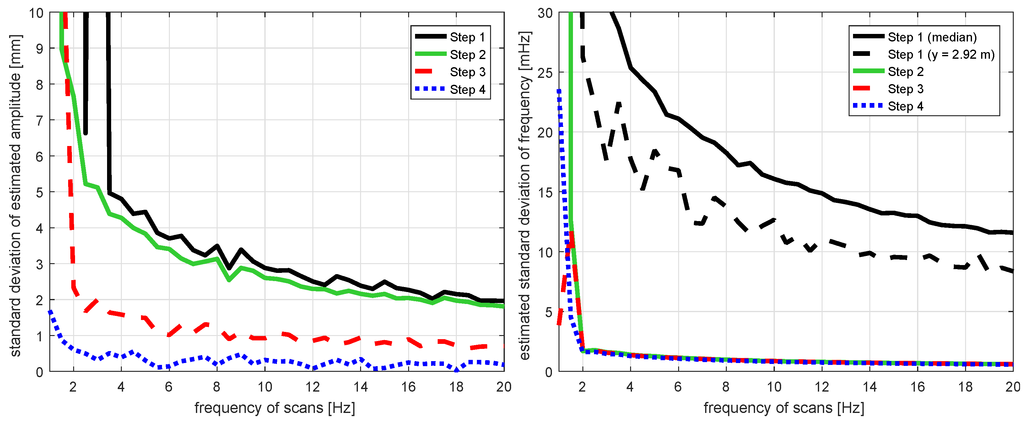
We compare the results of the different set-ups along the variation of the sampling rate of the measurements from 1 Hz to 20 Hz leading to 3 to 59 measured profiles with a fixed observation length of 3 s (Table 2). In all previous simulations, the sampling rate equaled 4 Hz. For the analysis, we use the same quantities as in the previous subsection.
Figure 8 depicts the results. In general, high agreements with the results for varying observations lengths are visible. On the one hand, this is not surprising, as in this case, the number of observations is increased again, but by higher sampling rates. On the other hand, differences occur to the previous subsection as the higher sampling rates increase the number of measurements per oscillation period. Apart from the already made statements, the following results can be observed:
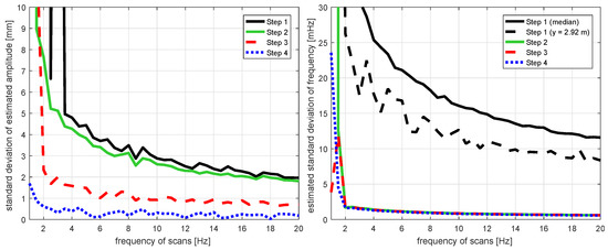
Figure 8.
Results of set-up “sampling rate”: standard deviation of amplitude (left) and frequency (right). For reasons of clarity, the vertical axes are limited to 10 mm or 30 mHz, respectively, although larger values exist.
- In step 4, a sampling rate of about 3 Hz is already sufficient for estimating a precise amplitude. Higher frequencies do not improve the estimation significantly. For step 3, this is the case at about 6 Hz. For steps 1 and 2, the uncertainty decreases up to 20 Hz.
- The amplitudes’ standard deviations of steps 1 and 2 are similar for all frequencies. The one of step 3 is about 60% smaller, the one of step 4 is about 85% smaller at a sampling rate of 20 Hz.
- The uncertainty in the estimated frequency decreases for all steps with the increase of the sampling rate of the laser scanner, but the benefit is small for steps 2, 3 and 4 starting from about 10 Hz.
- The improvements of using the spatio-temporal models with steps 2, 3 and 4 compared to the standard procedure with step 1 are minimally 90% for the frequency.
The first statement can also be related numerically to the previous subsection and the variation of the observation length—for step 3, an equilibrium state for the standard deviation of the estimated amplitude is reached with a minimal number of about 20 profiles; for step 4, this is the case for about 10 profiles. Regarding the variation of the sampling rate, those equilibrium states are reached for minimal sampling rates of 6 Hz (step 3) or 3 Hz (step 4), respectively. These conclusions resemble each other in the fact that equilibrium states are reached at a minimal number of about 6400 … 7000 measurements for step 3 or a minimal number of about 3200 … 3500 measurements for step 4.
Disregarding these general trends, small oscillations in the standard deviations are also visible in Figure 8. These are due to the simulation environment and the inevitable interference of sampling frequency, oscillation frequency and the pseudo-random process of the generated measurement noise.
5.4. Variation of Spatial Point Distance
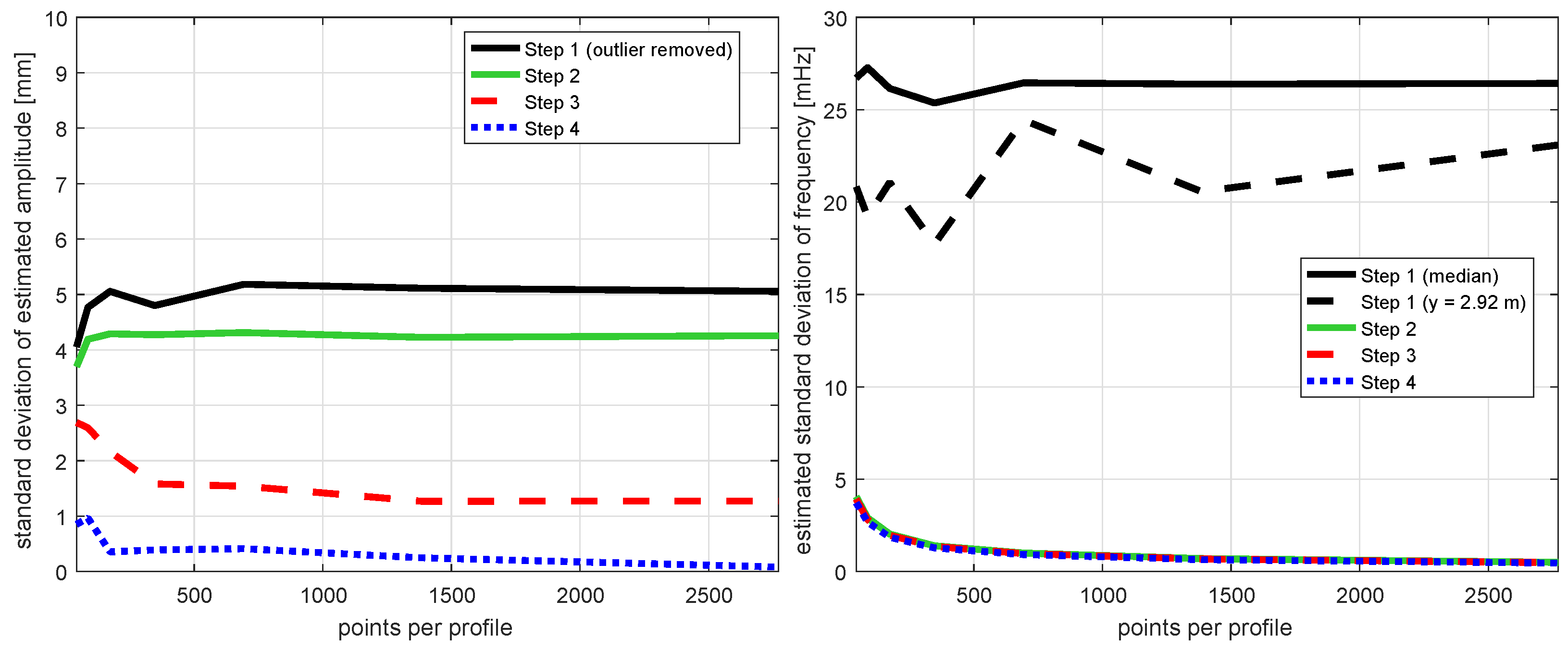
As last set-up, the spatial point distance is varied within the simulation starting from 43 points per profile—leading to a spatial point distance of 227 mm—and ending at 2771 points per profile—leading to a spatial point distance of 4 mm. The observation length remains at 3 s, the sampling rate at 4 Hz (Table 2). In general, we can state the following based on Figure 9 left:
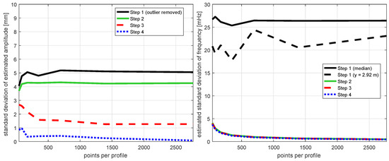
Figure 9.
Results of set-up “point distance”: standard deviation of amplitude (left) and frequency (right). For reasons of clarity, the vertical axes are limited to 10 mm or 30 mHz, respectively.
- The uncertainty of the estimated amplitude does rarely depend on the number of points on the profile.
- For step 1, this is straightforward since each measured position is processed individually and independent from the neighbored points. The fact that the shown standard deviations are not identical for step 1 is explainable by the fact that we deal with stochastic processes here. The fluctuation are not significant.
- For step 2, the variation is also insignificant since the spatial connection in this step is only related to the frequency, not the amplitude (Equation (4)).
- For steps 3 and 4, the uncertainty only slightly decreases with a larger amount of points on the profile. This decrease is—starting from about 4000 points on the profile—rather small compared to the effect of the observation length and the sampling rate.
The effect on the estimated frequency is shown in Figure 9 right: Again, the variation for step 1 can be assigned to the stochasticity of the underlying process. The variation is larger for the single position at m since only one single measurement position is used for its estimation. The standard deviations for the frequencies at steps 2, 3 and 4 are again—similarly to Figure 7 right and Figure 8 right—identical and by many factors smaller than the one of step 1.
6. Discussion of the Results
The results imply that a spatio-temporal modelling has a large impact on the results of the vibration monitoring. Before discussing the results, we evaluate the significance of the previous results:
- While the results have been analyzed here only for the estimated amplitude and the estimated frequency, the results can be transferred to the other estimated parameters: the mean value and the phase.
- The analysis is also limited here to one oscillation scenario with fixed geometry and only slightly varying conditions realized by different set-ups. Thus, the concrete numeric values shown in the figures before are not of highest relevance; but the conclusion drawn can also be transferred to different scenarios.
- Finally, the performed analysis is bounded by the four steps of spatio-temporal models that are developed. Other models could have been also realized, for example, using B-splines or other curves for modelling the spatial trend [15,56]. However, the purpose of this study is to introduce new strategies for connecting spatially distributed measurements in vibration monitoring. The general benefit—as shown here—is independent from the detailed realization of individual functional and stochastic models. In reality, these have to be applied to the specific structure, anyway.
Based on the results of Section 4 and Section 5, we highlight several aspects concerning the general applicability of spatio-temporal models:
- By including spatial connections between the oscillations measured at different positions on a structure, the redundancy and the reliability, that is, the ability to estimate unbiased parameters, increases.
- Spatial connections can be introduced in the modelling using solely the functional model—as has been done in steps 2 and 4 with different complexity—or also the stochastic model—as has been done in step 3—by using, for example, pseudo observations.
- Spatial connections for individual parameters decrease mostly only the uncertainty of these individual parameters in the parameter estimation. Thus, firstly, step 2 (spatial connection for frequency and phase) does not overall improve the estimation of the amplitude on the complete beam of the structure, just at some parts (Figure 5). Secondly, the results for the estimated frequency are similar for steps 2, 3 and 4 after a certain convergence since all steps model the frequency identically (Figure 6, Figure 7 right, Figure 8 right, Figure 9 right). Regarding the amplitude, larger differences are visible (Figure 5, Figure 7 left, Figure 8 left, Figure 9 left).
The general conclusion that a higher redundancy improves a least-squares estimate might be apparent. Anyway, the relevance of this study rests upon the fact that we reveal the individual benefit of different strategies for obtaining higher redundancy in the parameter identification process.
Concerning the four main questions of this present study (see Section 1), we provide the following answers:
- 1.
- Spatio-temporal models can be formulated using functional or stochastic connections between the dynamic behavior of spatially neighbored parts of the oscillating structure.
- 2.
- The observation length can be reduced noticeably if using spatio-temporal models, still maintaining an uncertainty that is by many factors lower compared to not connecting neighbored measurement positions. Thus, changes in the vibration parameters, for example, due to changing ambient influences, are faster visible in the results if using spatio-temporal models.
- 3.
- The sampling rate can be reduced noticeably if using spatio-temporal models where the level of uncertainty is generally by many factors lower for these spatio-temporal models, independent from the sampling rate within a certain range.
- 4.
- The effect of a high spatial point density is rather small compared to the one of the sampling rate and the observation length. Thus, the spatial distance between the measured positions on the structure does not need to be small to achieve results that are improved compared to using no spatio-temporal models. This holds, of course, under the assumption of homogeneous material and mechanical properties of the structure.
These results have an impact on the rules of vibration monitoring or time series analysis in general. Firstly, the Nyquist frequency
determines the maximal frequency that can be reconstructed based upon a given measurement frequency or sampling rate , respectively [12]. Consequently, since the true oscillation frequency equals Hz here, the measurement frequency—at each individual measurement position—has to be at least Hz. Figure 8 indeed implies that, for the estimated frequencies, sampling rates of minimally 2 Hz should be used for all steps of the spatio-temporal models. However, for the estimated amplitudes, step 4 would also work properly with the minimal frequency of 1 Hz that was implemented.
Apparently, the spatio-temporal connection of the measurements reduces the demand for a high sampling rate at each individual measurement position. Instead, thee need for a high temporal sampling rate fulfilling the requirement of the Nyquist frequency can be substituted by a high spatial sampling rate. Consequently, the Nyquist frequency condition cannot be automatically linked only with the sampling frequency of one sensor but also needs to account for the spatial sampling rate as well if using spatio-temporal models. Already [57] interpreted the Nyquist frequency spatially.
Secondly, the observation length should usually be minimally about five times longer than the period of the oscillation is for sharply estimating the included frequencies following the leakage effect [12,13]. In vibration monitoring, this is always fulfilled since the vibrations are high-frequent oscillations so that observation lengths do not need to be longer than several seconds. However, from methodological site and also regarding the oscillation of slowly deforming structures due to sun exposure, for instance, this is highly relevant.
Considering an oscillation frequency of Hz, the period of one oscillation equals 1.4 s so that 5 periods have a length of 7 s equaling a number of about 25 measured profiles in this simulation. Figure 7 implies that the spatio-temporal model of step 4 is already able to estimate precise parameters with about 10 profiles (amplitude and frequency). Thus, analogous to the Nyquist frequency, the minimal number of five observed oscillation periods is also not only linked to the observation length but also to the spatial sampling rate if using spatio-temporal models.
7. Conclusions and Outlook
Vibration monitoring is a frequent task within the general topic of Structural Health Monitoring. For this monitoring, usually accelerometers, strain gauges, fibre optic sensors or GNSS receivers are placed on pre-selected positions on the structure and the point-wise measurements are individually processed to estimate the relevant modal parameters, for example, oscillating amplitudes and natural frequencies. In this study, we present a concept to model the vibrations spatio-temporally using different steps of complexity. While those models are indispensable if using profile laser scanners for vibration monitoring considering their measurement properties (temporally varying measurement positions, no pre-selection of measurement positions, no simultaneous measurements at different measurement positions), they can also be used for vibration monitoring based on the other mentioned sensors.
The evaluation of the introduced spatio-temporal models reveals that they allow an improved parameter estimation compared to the usually used strategies—even at lower measurement frequencies and shorter observation lengths. This is because the spatial sampling of the structures includes further information into the parameter estimation. To consider the Nyquist frequency and potential leakage effects at vibration monitoring, the spatial sampling has, thus, also to be involved additionally to the temporal sampling.
Up to now, this study rests upon simulations and the vibration monitoring of elongated structures along one single extent. We will apply these methods to real world examples and also expand it to the vibration monitoring of structures with an extent in two dimensions using 3D laser scanning.
Author Contributions
Conceptualization, C.H. and H.N.; methodology, C.H. and H.N.; implementation and analysis, C.H.; writing—original draft preparation, C.H.; writing—review and editing, C.H. and H.N. All authors have read and agreed to the published version of the manuscript.
Funding
This research received no external funding.
Conflicts of Interest
The authors declare no conflict of interest.
References
- Brownjohn, J.M.W.; Stefano, A.D.; Xu, Y.L.; Wenzel, H.; Aktan, A.E. Vibration-based monitoring of civil infrastructure: Challenges and successes. J. Civ. Struct. Health Monit. 2011, 1, 79–95. [Google Scholar] [CrossRef]
- Marcheggiani, L.; Clement, F.; Formisano, A. Static and dynamic testing of highway bridges: A best practice example. J. Civ. Struct. Health Monit. 2020, 10, 43–56. [Google Scholar]
- Sabato, A.; Niezreck, C.; Fortino, G. Wireless MEMS-Based Accelerometer Sensor Boards for Structural Vibration Monitoring: A Review. IEEE Sens. J. 2016, 17, 226–235. [Google Scholar] [CrossRef]
- Whelan, M.J.; Gangone, M.V.; Janoyan, K.D.; Jha, R. Wireless Vibration Monitoring for Damage Detection of Highway Bridges. In Proceedings of the SPIE—The International Society for Optical Engineering, San Diego, CA, USA, 9–13 March 2008. [Google Scholar]
- Abir, J.; Longo, S.; Morantz, P.; Shore, P. Optimized estimator for real-time dynamic displacement measurement using accelerometers. Mechatronics 2016, 39, 1–11. [Google Scholar] [CrossRef]
- Hale, J.M.; Chapman, M.M. Design, installation and calibration of a strain gauge structural monitoring system for a timber windmill. Exp. Tech. 2014, 38, 45–53. [Google Scholar] [CrossRef]
- Zhang, B.; Benmokrane, B.; Nicole, J.; Masmoudi, R. Evaluation of fibre optic sensors for structural condition monitoring. Mater. Struct. 2002, 35, 357–364. [Google Scholar] [CrossRef]
- De Oliveira, J.V.M.; Larocca, A.P.C.; de Araujo Neto, J.O.; Cunha, A.L.; dos Santos, M.C.; Schaal, R.E. Vibration monitoring of a small concrete bridge using wavelet transforms on GPS data. J. Civ. Struct. Health Monit. 2019, 9, 397–409. [Google Scholar] [CrossRef]
- Yu, J.; Meng, X.; Yan, B.; Xu, B.; Fan, Q.; Xie, Y. Global Navigation Satellite System-based positioning technology for structural health monitoring: A review. Struct. Control Health Monit. 2020, 27, e2467. [Google Scholar] [CrossRef]
- Carden, E.P.; Fanning, P. Vibration Based Condition Monitoring: A Review. Struct. Health Monit. 2004, 3, 355–377. [Google Scholar] [CrossRef]
- Venglar, M.; Sokol, M.; Aroch, R. Ambient vibration measurements of steel truss bridges. J. Meas. Eng. 2018, 6, 234–239. [Google Scholar] [CrossRef]
- Priestley, M. Spectral Analysis and Time Series: 1 (Probability and Mathematical Statistics); Academic Press Inc.: San Diego, CA, USA, 1981. [Google Scholar]
- Heunecke, O.; Kuhlmann, H.; Welsch, W.; Eichhorn, A.; Neuner, H. Hanbuch Ingenieurgeodäsie. Auswertung Geodätischer Überwachungsmessungen, 2nd ed.; Wichmann: Heidelberg, Germany, 2013.
- Kutterer, H.; Paffenholz, J.A.; Vennegeerts, H. Kinematisches terrestrisches Laserscanning. Z. Vermesungswesen 2009, 134, 79–87. [Google Scholar]
- Schill, F.; Eichhorn, A. Deformation Monitoring of Railway Bridges with a Profile Laser Scanner. Z. Vermessungswesen 2019, 2, 109–118. [Google Scholar]
- Doebling, S.W.; Farrar, C.R.; Prime, M.B.; Shevitz, D.W. Damage Identification and Health Monitoring of Structural and Mechanical Systems from Changes in Their Vibration Characteristics: A Literature Review; LA-13070-MS, UC-900; Los Alamos National Laboratory: Los Alamos, NM, USA, 1996. [Google Scholar]
- Catbas, F.N.; Aktan, A.E.; Kijewski-Correa, T. Structural Identification of Constructed Facilities. Approaches, Methods and Technologies for Effective Practice of St-id; American Society of Civil Engineers (ASCE): Reston, VA, USA, 2013. [Google Scholar]
- Boscato, G.; Fragonara, L.Z.; Cecchi, A.; Reccia, E.; Baraldi, D. Structural Health Monitoring through Vibration-Based Approaches. Shock Vib. 2019, 2019, 2380616. [Google Scholar] [CrossRef]
- Brownjohn, J.M.W.; Pan, T.C. Response of tall buildings to weak long distance earthquakes. Earthq. Eng. Struct. Dyn. 2001, 30, 709–729. [Google Scholar] [CrossRef]
- Paziewski, J.; Wielgosz, P.; Elgosz, P.; Sieradzki, R.; Baryla, R. Detection of structural vibration with high-rate GNSS Precise Point Positioning methodology and case study results. In Proceedings of the 4th Joint International Symposium on Deformation Monitoring (JISDM), Athens, Greece, 15–17 May 2019. [Google Scholar]
- Yigit, C.O.; Dindar, A.A.; El-Mowafy, A.; Bezcioglu, M.; Gikas, V. Investigating the ability of high-rate GNSS-PPP for determining the vibration modes of engineering structures: Small scale model experiment. In Proceedings of the 4th Joint International Symposium on Deformation Monitoring (JISDM), Athens, Greece, 15–17 May 2019. [Google Scholar]
- Roberts, G.W.; Brown, C.J.; Tang, X.; Meng, X.; Ogundipe, O. A Tale of Five Bridges; the use of GNSS for Monitoring the Deflections of Bridges. J. Appl. Geod. 2014, 8, 241–263. [Google Scholar] [CrossRef]
- Gikas, V.; Mpimis, T.; Piniotis, G.; Perakis, H.; Papadimitriou, F.; Drimeris, K.; Sotiriou, P. Long-term monitoring of the Tall Piers of a Multi-span Beam Bridge Using a Network of Digital Inclinometers: First Results and Perspectives. In Proceedings of the 4th Joint International Symposium on Deformation Monitoring (JISDM), Athens, Greece, 15–17 May 2019. [Google Scholar]
- Holst, C.; Burghof, M.; Kuhlmann, H. Modeling the beam deflection of a gantry crane under load. J. Surv. Eng. 2014, 140, 52–59. [Google Scholar] [CrossRef]
- Neitzel, F.; Niemeier, W.; Weisbrich, S.; Lehmann, M. Investigation of low-cost accelerometer, terrestrial laser scanner and ground-based radar interferometer for vibration monitoring of bridges. In Proceedings of the 6th European Workshop on Structural Health Monitoring, Dresden, Germany, 3–6 July 2012. [Google Scholar]
- Lienhart, W.; Erhart, M.; Grick, M. High frequent total station measurements for the monitoring of bridge vibrations. J. Appl. Geod. 2017, 11, 1–8. [Google Scholar] [CrossRef]
- Paar, R.; Marendić, A.; Wagner, A.; Wiedemann, W.; Wunderlich, T.; Roic, M.; Damjanovic, D. Using IATS and digital levelling staffs for the determination of dynamic displacements and natural oscillation frequencies of civil engineering structures. In Proceedings of the Conference Proceedings INGEO 2017 7th International Conference on Engineering Surveying, Lisbon, Portuga, 18–20 October 2017. [Google Scholar]
- Rytter, A. Vibration Based Inspection of Civil Engineering Structures. Ph.D. Thesis, Department of Building Technology, Aalborg University, Aalborg, Denmark, 1993. [Google Scholar]
- Deraemaeker, A.; Reynders, E.; De Roeck, G.; Kullaa, J. Vibration-based structural health monitoring using output-only measurements under changing environment. Mech. Syst. Signal Process. 2008, 22, 34–56. [Google Scholar] [CrossRef]
- Peeters, B.; Maeck, J.; Roeck, G.D. Vibration-based damage detection in civil engineering: Excitation sources and temperature effects. Smart Mater. Struct. 2001, 10, 518–527. [Google Scholar] [CrossRef]
- Ogundare, J.O. Precision Surveying. The Principles and Geomatics Practice; John Wiley & Sones: Hoboken, NJ, USA, 2015. [Google Scholar]
- Liu, W.; Chen, S.E. Reliability analysis of bridge evaluations based on 3D Light Detection and Ranging data. Struct. Control Health Monit. 2013, 20, 1397–1409. [Google Scholar] [CrossRef]
- Mosalam, K.M.; Takhirov, S.M.; Park, S. Applications of laser scanning to structures in laboratory tests and field surveys. Struct. Control Health Monit. 2014, 21, 115–134. [Google Scholar] [CrossRef]
- Sanchez-Rodriguez, A.; Riveiro, B.; Conde, B.; Soilan, M. Detection of structural faults in piers of masonry arch bridges through automated processing of laser scanning data. Struct. Control Health Monit. 2018, 25, e2126. [Google Scholar] [CrossRef]
- Cabaleiro, M.; Riveiro, B.; Arias, P.; Caamano, J.C. Algorithm for the analysis of deformations and stresses due to torsion in a metal beam from LIDAR data. Struct. Control Health Monit. 2016, 23, 1032–1046. [Google Scholar] [CrossRef]
- Holst, C.; Schunck, D.; Nothnagel, A.; Haas, R.; Wennerbäck, L.; Olofsson, H.; Hammargren, R.; Kuhlmann, H. Terrestrial laser scanner two-face measurements for analyzing the elevation dependent deformation of the Onsala Space Observatory 20-m radio telescope’s main reflector in a bundle adjustment. Sensors 2017, 17, 1833. [Google Scholar] [CrossRef] [PubMed]
- Holst, C.; Nothnagel, A.; Haas, R.; Kuhlmann, H. Investigating the gravitational stability of a radio telescope’s reference point using a terrestrial laser scanner: Case study at the Onsala Space Observatory 20-m radio telescope. ISPRS J. Photogramm. 2019, 149, 67–76. [Google Scholar] [CrossRef]
- Jaafar, H.A.; Meng, X.; Sowter, A.; Bryan, P. New approach for monitoring historic and heritage buildings: Using terrestrial laser scanning and generalised Procrustes analysis. Struct. Control Health Monit. 2017, 24, e1987. [Google Scholar] [CrossRef]
- Bassoli, E.; Vincenzi, L.; D’Altri, A.M.; de Miranda, S.; Forghieri, M.; Castellazzi, G. Ambient vibration-based finite element model updating of an earthquake-damaged masonry tower. Struct. Control Health Monit. 2018, 25, e2150. [Google Scholar] [CrossRef]
- Dai, K.; Li, A.; Zhang, H.; Chen, S.E.; Pan, Y. Surface damage quantification of postearthquake building based on terrestrial laser scan data. Struct. Control Health Monit. 2018, 25, e2210. [Google Scholar] [CrossRef]
- Neuner, H.; Holst, C.; Kuhlmann, H. Overview on Current Modelling Strategies of Point Clouds for Deformation Analysis. Allg. Vermess. Nachrichten 2016, 2016, 328–339. [Google Scholar]
- Law, D.W.; Silcock, D.; Holden, L. Terrestrial laser scanner assessment of deteriorating concrete structures. Struct. Control Health Monit. 2018, 25, e2156. [Google Scholar] [CrossRef]
- Lee, J.; Lee, K.C.; Lee, S.; Lee, Y.J.; Sim, S.H. Long-term displacement measurement of bridges using a LiDAR system. Struct. Control Health Monit. 2019, 26, e2428. [Google Scholar] [CrossRef]
- Hesse, C.; Neuner, H.; Kutterer, H. Statistical Analysis of Kinematic Laser Scans. In Proceedings of the Optical 3-D Measurements Techniques VII, Vienna, Austria, 3–5 October 2005. [Google Scholar]
- Chen, D.M.; Zhu, W.D. Rotating Machinery, Vibro-Acoustics & Laser Vibrometry. In Volume 7, Conference Proceedings of the Society for Experimental Mechanics Series; Chapter Rapid and Dense 3D Vibration Measurement by Three Continuously Scanning Laser Doppler Vibrometers; Springer: Cham, Switzerland, 2019. [Google Scholar]
- Stanbridge, A.; Ewins, D. Modal testing using a scanning laser doppler vibrometer. Mech. Syst. Signal Process. 1999, 13, 255–270. [Google Scholar] [CrossRef]
- Gentile, C.; Bernardini, G. Output-only modal identification of a reinforced concrete bridge from radar-based measurements. Ndt E Int. 2008, 41, 544–553. [Google Scholar] [CrossRef]
- Aryan, P.; Kotousov, A.; Ng, C.T.; Cazzolato, B.S. A baseline-free and non-contact method for detection and imaging of structural damage using 3D laser vibrometry. Struct. Control Health Monit. 2017, 24, e1894. [Google Scholar] [CrossRef]
- Rana, S.; Nagayama, T.; Hisazumi, K.; Tominaga, T. Damage identification of a belt conveyor support structure based on cross-sectional vibration characteristics. Struct. Control Health Monit. 2019, 26, e2349. [Google Scholar] [CrossRef]
- Chen, D.; Xu, Y.; Zhu, W.D. Damage Identification of Beams Using a Continuous Scanning Laser Doppler Vibrometer System. J. Vib. Acoust. 2016, 138. [Google Scholar] [CrossRef]
- Ubertini, F.; Gentile, C.; Materazzi, A.L. Automated modal identification in operational conditions and its application to bridges. Eng. Struct. 2013, 46, 264–278. [Google Scholar] [CrossRef]
- Aloisio, A.; Pasca, D.P.; Alaggio, R.; Fragiacomo, M. Bayesian estimate of the elastic modulus of concrete box girders from dynamic identification: A statistical framework for the A24 motorway in Italy. Struct. Infrastruct. Eng. 2020, 1–13. [Google Scholar] [CrossRef]
- Zoller+Froehlich. Zoller + Froehlich Imager 9012 Data Sheet. Available online: www.zf-laser.com (accessed on 4 February 2020).
- Heinz, E.; Mettenleiter, M.; Kuhlmann, H.; Holst, C. Strategy for determining the stochastic distance characteristics of the 2D laser scanner Z+F Profiler 9012A with special focus on the close range. Sensors 2018, 18, 2253. [Google Scholar] [CrossRef]
- Mikhail, E.; Ackermann, F. Observations and Least Squares; Dun-Donelly: New York, NY, USA, 1976. [Google Scholar]
- Förstner, W.; Wrobel, B. Photogrammetric Computer Vision: Statistics, Geometry, Orientation and Reconstruction; Springer International Publishing: Cham, Switzerland, 2016. [Google Scholar]
- Holst, C.; Eling, C.; Kuhlmann, H. Automatic optimization of height network configurations for detection of surface deformations. J. Appl. Geod. 2013, 7, 103–113. [Google Scholar] [CrossRef]
Publisher’s Note: MDPI stays neutral with regard to jurisdictional claims in published maps and institutional affiliations. |
© 2021 by the authors. Licensee MDPI, Basel, Switzerland. This article is an open access article distributed under the terms and conditions of the Creative Commons Attribution (CC BY) license (https://creativecommons.org/licenses/by/4.0/).

