Sea Ice Thickness Estimation Based on Regression Neural Networks Using L-Band Microwave Radiometry Data from the FSSCat Mission

Abstract

Several methods have been developed to provide polar maps of sea ice thickness (SIT) from L-band brightness temperature (T${}_B$) and altimetry data. Current process-based inversion methods to yield SIT fail to address the complex surface characteristics because sea ice is subject to strong seasonal dynamics and ice-physical properties are often non-linearly related. Neural networks can be trained to find hidden links among large datasets and often perform better on convoluted problems for which traditional approaches miss out important relationships between the observations. The FSSCat mission launched on 3 September 2020, carries the Flexible Microwave Payload-2 (FMPL-2), which contains the first Reflected Global Navigation Satellite System (GNSS-R) and L-band radiometer on board a CubeSat—designed to provide T${}_B$ data on global coverage for soil moisture retrieval, and sea ice applications. This work investigates a predictive regression neural network approach with the goal to infer SIT using FMPL-2 T${}_B$ and ancillary data (sea ice concentration, surface temperature, and sea ice freeboard). Two models—covering thin ice up to 0.6 m and full-range thickness—were separately trained on Arctic data in a two-month period from mid-October to the beginning of December 2020, while using ground truth data derived from the Soil Moisture and Ocean Salinity (SMOS) and Cryosat-2 missions. The thin ice and the full-range models resulted in a mean absolute error of 6.5 cm and 23 cm, respectively. Both of the models allowed for one to produce weekly composites of Arctic maps, and monthly composites of Antarctic SIT were predicted based on the Arctic full-range model. This work presents the first results of the FSSCat mission over the polar regions. It reveals the benefits of neural networks for sea ice retrievals and demonstrates that moderate-cost CubeSat missions can provide valuable data for applications in Earth observation.

1. Introduction

Arctic sea ice reached its annual minimum extent in mid-September 2020, being the second lowest on record [1]. Continuous knowledge regarding the distribution of sea ice is particularly important for polar and mid-latitude climate monitoring [2]. Sea ice volume is an essential climate indicator that is required to understand the balances of mass and surface energy, which can be estimated through observations of sea ice thickness (SIT) and sea ice concentration (SIC). Multi-source data records of annual mean SIT—acquired from on-ice measurements, airborne and satellite-based observations—have proved that both SIT and the amount of multi-year ice in the Arctic have been decreasing by about one-third during the last 40 years [3]. Space-borne microwave radiometry observations over polar areas have been available since 1979, and data at low microwave frequencies can be collected independently of daylight and are widely unaffected by atmospheric conditions. Brightness temperature (T${}_B$) observations at L-band (∼1.4 GHz) are sensitive to thin sea ice up to ∼0.6 m [4,5]. SIT retrievals above 1 m have been successfully derived based on sea ice freeboard (Fb) estimates from satellite altimeters [6,7].

The European Space Agency’s (ESA) Soil Moisture and Ocean Salinity (SMOS) mission was launched in 2009 carrying on board the Microwave Imaging Radiometer with Aperture Synthesis (MIRAS), the first spaceborne L-band interferometric radiometer [8,9]. MIRAS provides T${}_B$ data at global coverage with a revisit time at the equator of 1–3 days and a spatial resolution of ∼40 km. Several methods have been developed to estimate the distribution of thin SIT at Arctic scale while using SMOS T${}_B$ data at multiple incidence angles and polarizations [10,11]. A combined thermodynamic and radiative transfer model has been used to evaluate the variations of ice-physical properties, including temperature and salinity [12,13]. T${}_B$ polarization differences were combined in growth models, along with empirical assumptions on sea ice properties [14]. A thin SIT product was developed on the basis of retrievals from the SMOS and the Soil Moisture Active Passive (SMAP) missions (also operating at L-band) [15]. ESA’s CryoSat-2 mission was launched in 2010 and it provides ice-sheet elevation and Fb estimates from radar altimetry [16]. Since then, several approaches have been implemented to provide maps of Arctic SIT from CryoSat-2 altimetry data [17,18,19]. SMOS and CryoSat-2 observations were merged according to their sensitivity ranges and uncertainties in a combined method to generate weekly Arctic full-range SIT [20,21].

Process-based retrieval algorithms to infer SIT rely on strong model assumptions and empirically determined sea ice properties. These simplifications are required due to sparsely available validation data and limited knowledge on the distribution of sea ice, exhibiting large spatio-temporal variability. Passive microwave sensors often do not capture all of the necessary information about SIT, but they also require ancillary data. The main uncertainties originate from long revisit times and large spatial resolution of satellites. Current SIT products show sufficient accuracy during the Arctic freeze-up period from mid-October to mid-March, but they do not perform well during the Arctic melting season.

Machine learning algorithms can often perform better on complex problems for which traditional approaches miss out hidden links between the model parameters among large amounts of data. They have been successfully applied to segment sea ice based on the distribution of surface signatures of satellite observations to recognize patterns of sea ice properties among different scales [22,23,24]. Data-driven approaches, such as neural networks (NN), were developed decades ago, and they can adapt to new ice conditions such as changing sea ice types and intermittent periods of freeze up and melting. Before Arctic-wide L-band observations from SMOS were available, NNs were used to infer SIT based on SIC maps from satellite radiometry observations at higher bands, and ancillary geophysical parameters, such as surface air temperature and ice drift velocity [25]. The time series of SIC maps were analyzed on the basis of NNs to forecast SIC by assessing the time-varying characteristics of previous observations [26,27]. Snow depth is an important factor with regard to the inference of SIT from both microwave radiometry and freeboard observations, and its estimation is particularly complicated due to the complexity of the radiation properties of the snow layer. Therefore, regression NN approaches have been developed to invert snow depth using data from multi-frequency satellite microwave radiometer measurements, including the Special Sensor Microwave Imager (SSM/I), the Scanning Multi-channel Microwave Radiometer (SMMR), the Advanced Microwave Scanning Radiometer 2 (AMSR2), and SMOS [28,29,30,31]. NNs are efficient and often easy to implement. They have the advantage to be capable of recognizing the principal forcing mechanisms contained in the non-linear relationships between geophysical parameters, and they can provide similar or better results when compared to those of conventional models.

There are only few satellite missions available that are suitable for providing sufficient coverage to retrieve SIT at polar scale. The new Copernicus Imaging Microwave Radiometer (CIMR) mission, which is expected to be launched after 2025, is planned to follow up the SMOS and SMAP missions providing data continuity with at least daily revisit in the polar regions [32,33].

Today, nanosatellite technology has reached the maturity to perform scientific missions, and the number of deployed instruments has grown steadily over the past decade [34,35]. CubeSats are miniature satellites that are composed of small unit cubes (U) of 10 × 10 × 10 cm${}^3$, with a maximum weight of 1.33 kg. Their payloads have an advantage over those carried by traditional missions (i.e., large passive optical and microwave payloads), due to their smaller dimensions in terms of size, mass, power consumption, and downlink capability. Markedly reduced expenses in development, construction, and satellite launch make them more accessible to universities and research institutes, and their use is on the rise to expand the field of applications in Earth observation. Commercial companies, such as ‘Planet’ and ‘Spire’, operate constellations of hundreds of 3-U CubeSats (∼30 × 10 × 10 cm${}^3$), carrying optical imagers or GNSS-Radio Occultation payloads [36,37].

The FSSCat mission, launched on 3 September 2020, is formed by two federated CubeSats, with one of them (${}^3$Cat-5/A) carrying the Flexible Microwave Payload-2 (FMPL-2) on board, a combined Reflected Global Navigation Satellite System (GNSS-R) radiometer and the first radiometer operating at L-band ever deployed on a CubeSat [38]. It is designed to provide maps of sea ice extent (SIE) and SIT over both poles on a five-day basis and soil moisture over land at low-moderate resolution, and it is the first CubeSat mission contributing to the Copernicus system (Land and Marine Environment Monitoring Services). Both of the FMPL-2 instruments have been successfully validated in orbit and the first set of nominal acquisitions are available from 1–13 October 2020 [39].

This work investigates predictive regression NN frameworks to infer SIT based on the first FMPL-2 T${}_B$ acquisitions provided by the FSSCat mission. To do so, two separate NNs were implemented to generate Arctic and Antarctic SIT maps by combining FMPL-2 T${}_B$ data from the FSSCat mission with ancillary maps of SIC from the European Organisation for the Exploitation of Meteorological Satellites (EUMETSAT), and skin temperature provided by the European Centre for Medium-Range Weather Forecasts (ECMWF). The first model is devoted to model thin SIT up to 0.6 m while using a thin sea ice product derived from SMOS (SIT${}_{SMOS}$) as ground truth. The second network is designed to model full-range SIT. Input data are further complemented by CryoSat-2 Fb estimates to extend the previous model, using a merged product derived from CryoSat-2 and SMOS (SIT${}_{CS2SMOS}$) as ground truth. Both of the SIT models are trained during the period from 15 October to 4 December 2020, and allowed to generate weekly composite maps of Arctic thin and full-range SIT. The Arctic dataset that was used to train the full-range model was compared to the same set of observations collected over Antarctic sea ice in terms of its variable ranges and densities. Because the Arctic training data encompasses most parts of the Antarctic dataset, the prediction of Antarctic sea ice based on the Arctic model was considered to be reasonable in statistical terms. The full-range model was applied to Antarctic data in an initial attempt to provide monthly composite maps of Antarctic SIT.

2. Data and Methods

This section describes the satellite input features, and the implementation of the predictive regression NN models. In Section 2.1, the FSSCat mission and the Flexible Microwave PayLoad (FMPL-2) T${}_B$ data are presented. The selected set of ancillary data comprising SIC, surface temperature (T${}_S$), sea ice Fb, and the ground truth SIT datasets are described in Section 2.2. Section 2.3 explains the processing of the input features and the architecture of the NNs, which are separately trained under the optimization of the model hyperparameters to predict both thin SIT over the Arctic, and full-range SIT over the Arctic and Antarctic.

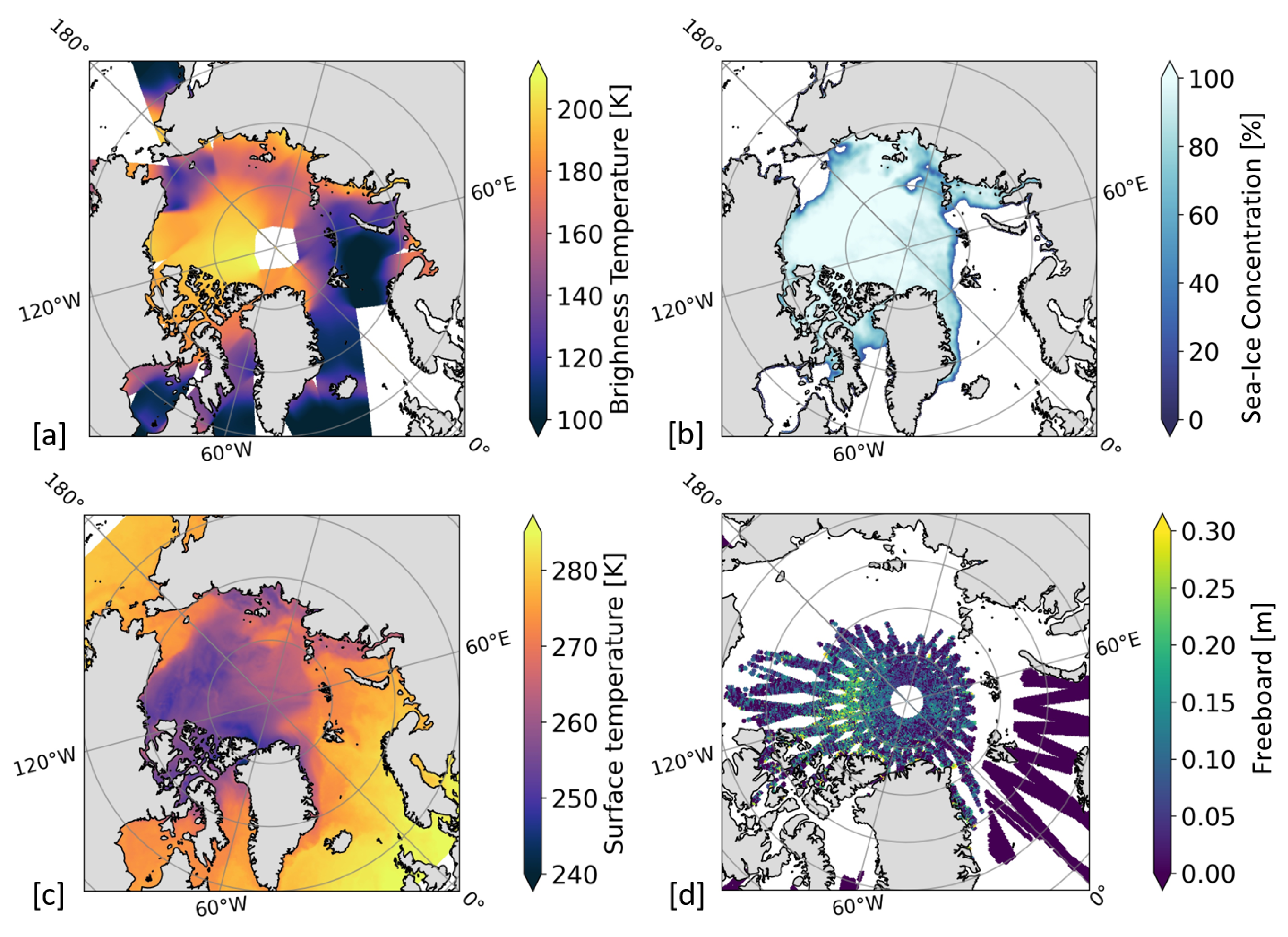
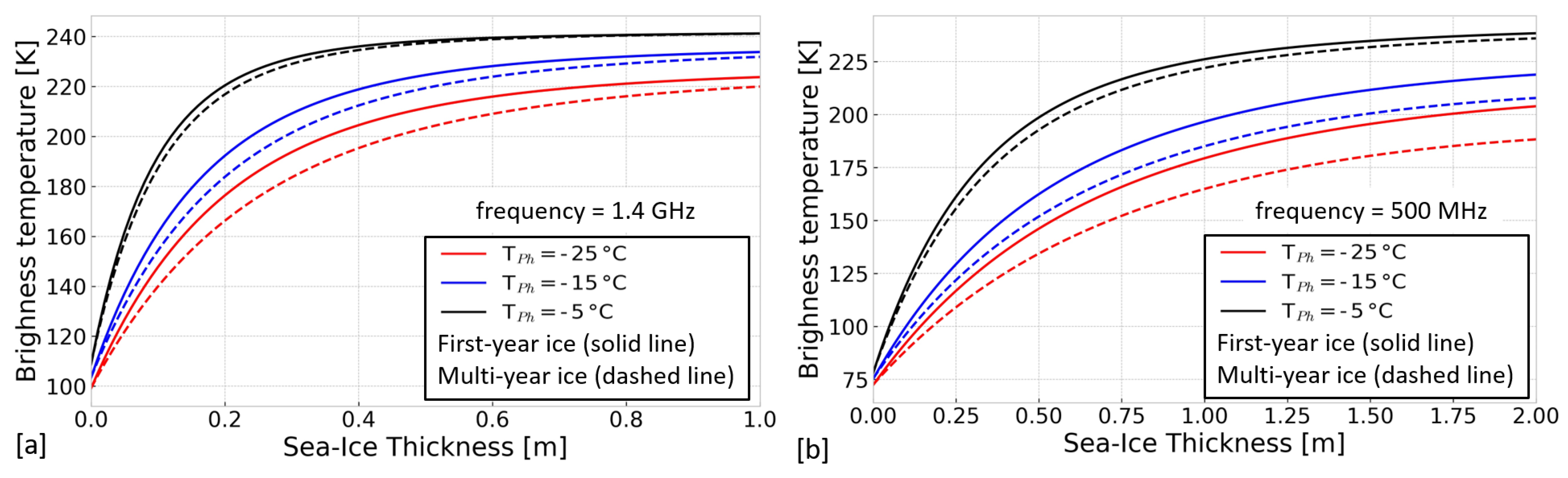
2.1. FMPL-2 Brightness Temperature Data from FSSCat

FSSCat is a tandem mission of two federated 6U CubeSats (${}^3$Cat-5/A and ${}^3$Cat-5/B) that was proposed by the Polytechnic University of Catalonia (UPC), and designed to retrieve geophysical data on SIE and SIT over polar areas, and low-resolution soil moisture content over land [38]. It was the winner of the 2017 ESA Small Sentinel Satellite Challenge and the overall Copernicus Masters Competition [40]. The two CubeSats were successfully launched on the VEGA Small Spacecraft Mission Service (SSMS) Proof of Concept (PoC) flight on 3 September 2020. Both of them comprise an Radio-Frequency (RF)/optical inter-satellite link payload and the ${}^3$Cat-5/A CubeSat carries the FMPL-2, a dual passive microwave remote sensing instrument that encompasses a Software-Defined Radio (SDR)-based GNSS-Reflectometer and an L-band radiometer with a nadir-pointing antenna and a footprint of ∼350 × 500 km${}^2$.

The radiometer acquires the antenna temperature, which represents the apparent T${}_B$ at almost global coverage at latitudes that range from ∼86° S to 86° N. All of the mission characteristics and the instrument and processing specifications are described in detail in [38,39]. T${}_B$ maps are constructed from single tracks under evaluation of the antenna pattern, and swath data were projected and regridded onto a 12.5 km Equal-Area Scalable Earth Grid (EASE-Grid 2.0) for both hemispheres using k-d-tree sampling—a fast nearest neighbor interpolation method to resample remote sensing images [41].

The major part of sea ice in the Northern Ocean occurs at 65° N northwards, whereas, in the Southern Ocean, excluding the Antarctic continent, it roughly extends between 60° S and 70° S, with fluctuating sea ice margins. Because ${}^3$Cat-5/A is a polar orbit satellite, its passes become denser towards the poles and produce more frequent overlaps. T${}_B$ maps can be acquired with sufficient coverage (>80$\%$ after filtering usable tracks) in less than five days and two complete consecutive maps can be obtained within three weeks. This allows for the production of weekly Arctic and monthly Antarctic SIT composite maps of the ice-covered areas, respectively. It is noteworthy that the revisit time could be further decreased if the satellite was able to operate with a larger duty cycle, or in the case more ${}^3$Cat-5/A-like CubeSats were added to the existing constellation. After the commissioning phase, data are available from 1 October to 4 December 2020. The observed period falls into the beginning of the Arctic freeze up, after sea ice having reached its annual minimum extent on 15 September 2020. Hereby, sea ice mainly consists of the remaining multi-year ice with an increasing amount of thin first-year ice. In contrast to the Arctic, the Southern Ocean melts and re-freezes almost completely on a yearly basis and it consists mainly of first-year ice. Sea ice around Antarctica had passed its maximum extent in September 2020, and it is declining during the observation period [42].

2.2. Ancillary Data

Ancillary data are included to assist the network in capturing useful information on the sea ice conditions at higher resolution. This enables the model to better address local SIT variability, which is supposed to be contained in the relationship between the input features. The availability of maps with sufficient temporal resolution with polar coverage and from both hemispheres was one requirement. Figure 1 visualizes maps of T${}_B$ and ancillary data as an example from 11 November 2020.

2.2.1. Sea Ice Concentration (SIC)

FMPL-2 T${}_B$ observations at the ocean-ice boundaries can be ambiguous, because their values partially consist of open water and sea ice. This often leads to an underestimation of thin ice, especially at low-concentrated areas around sea ice margins. The Ocean and Sea Ice Satellite Application Facility (OSI-SAF) OSI-401-b product by EUMETSAT provides SIC maps using a dynamic tie-point algorithm applied to T${}_B$ data from the Special Sensor Microwave Imager/Sounder (SSMIS) at 19 GHz and 37 GHz vertical, and at 37 GHz horizontal polarization [43]. The SIC maps are available on a daily basis at a 10 km Polar Stereographic grid projection true at 70° N/S for both hemispheres, respectively, and images can be downloaded from http://osisaf.met.no/p/ice/, (accessed on 07 February 2021). These maps were regridded to a 12.5 km EASE-Grid 2 to build a sea ice coverage mask. Only input data with a SIC > 15$\%$ were considered for training the network.

2.2.2. Surface Temperature (T${}_S$)

At microwave frequencies below 117 GHz, Planck’s law of electromagnetic radiation can be simplified using the Rayleigh–Jeans approximation, resulting in T${}_B$ being the product of the physical temperature (T${}_{Ph}$) and the ice emissivity with an error of <1$\%$ [44]. Hereby, the emissivity contains the actual information about the sea ice composition—including SIT—of the radiating layer. Figure 2 shows the relationship between T${}_B$ and SIT as a function of T${}_{Ph}$ and sea ice types that are based on a radiative transfer model considering two nadir-pointing observations at frequencies corresponding to L-band (1.4 GHz) and P-band (500 MHz), respectively. The model assumes a horizontally-layered column of sea ice above water (without snow on top) using empirically determined values for sea ice properties, such as salinity and surface roughness [45]. While the L-band signal already saturates around 0.6 m, the model reveals that observations at P-band contain information on SIT beyond 1.5 m and, in principle, they can be used to extent the sensitivity range of current retrieval algorithms. T${}_{Ph}$ can strongly vary among the pole areas and it has a gradient along the ice profile, which influences the penetration depth of the emitted signal at L-band. Additional physical properties, such as density and ice type, can further depend on the distribution of temperature, which makes a direct correction of T${}_{Ph}$ based on T${}_B$ complicated. The skin temperature (T${}_S$) product provided by the ECMWF represents the temperature value of the uppermost surface layer that satisfies the surface energy balance equation [46]. Daily T${}_S$ maps were considered to be relevant input features for model training. They were linearly interpolated to a 12.5 km EASE-Grid 2.0 for Northern and Southern hemispheres.

2.2.3. Sea Ice Freeboard (Fb)

The CryoSat-2 mission, which was launched by ESA in 2010, carries the Synthetic Aperture Radar (SAR) Interferometric Radar Altimeter (SIRAL) operating at Ku-band (∼13.6 GHz) to detect and monitor topograhical fluctuations and trends over land and sea ice [6,16]. A combination of elevation data with ancillary data, including sea ice type and snow depth and density, enables the estimation of sea ice Fb, i.e., the height of sea ice above sea level [47]. Cryosat-2 altimetry data have shown to be sensitive to SIT above 1 m, with increasing uncertainty for thinner ice [6]. Because Fb data contain information on the sea ice variability, predominantly thicker ice, it was considered to be a relevant input parameter to complement the L-band observations. Time series of the CryoSat-2 Level-2 SIRAL Geophysical Data Record 2 (GDR) full-orbit segments were projected onto a 12.5 km EASE-Grid 2.0 to generate daily Fb maps. The data are available for both hemispheres and they can be downloaded from https://science-pds.cryosat.esa.int/ (accessed on 7 February 2021) [48].

2.2.4. Sea Ice Thickness (SIT)

Two separate SIT products are selected as ground truth data in the neural network, covering the respective ranges of thin sea ice up to 0.6 m, and full-range SIT. Hereby, daily SMOS Level-3 SIT maps (SIT${}_{SMOS}$) are used for thin SIT retrieval [12], and weekly composites of the merged SMOS and CryoSat-2 Level-4 SIT maps (SIT${}_{CS2SMOS}$) were used to yield full-range SIT [21]. Both of the maps are obtained from SMOS L-band T${}_B$ measurements on the basis of a thermodynamic and a radiative transfer model considering the variations of ice-physical properties [10]. In the latter product, daily SMOS-derived SIT is combined in an optimal interpolation scheme with the weekly CryoSat-2 SIT. The SIT${}_{CS2SMOS}$ product contains information on surface height and sea ice Fb included in the different modes of the SIRAL Level-1b data. Both of the datasets are available from 2010 onwards at Arctic scale from mid-October to mid-April on a 25 km EASE-Grid 2.0 and they are provided by the Alfred Wegener Institute (AWI) for Polar and Marine Research. The data can be downloaded from https://smos-diss.eo.esa.int/socat/L3_SIT_Open, (accessed on 7 February 2021) and https://smos-diss.eo.esa.int/socat/L4_SIT_Open, (accessed on 7 February 2021).

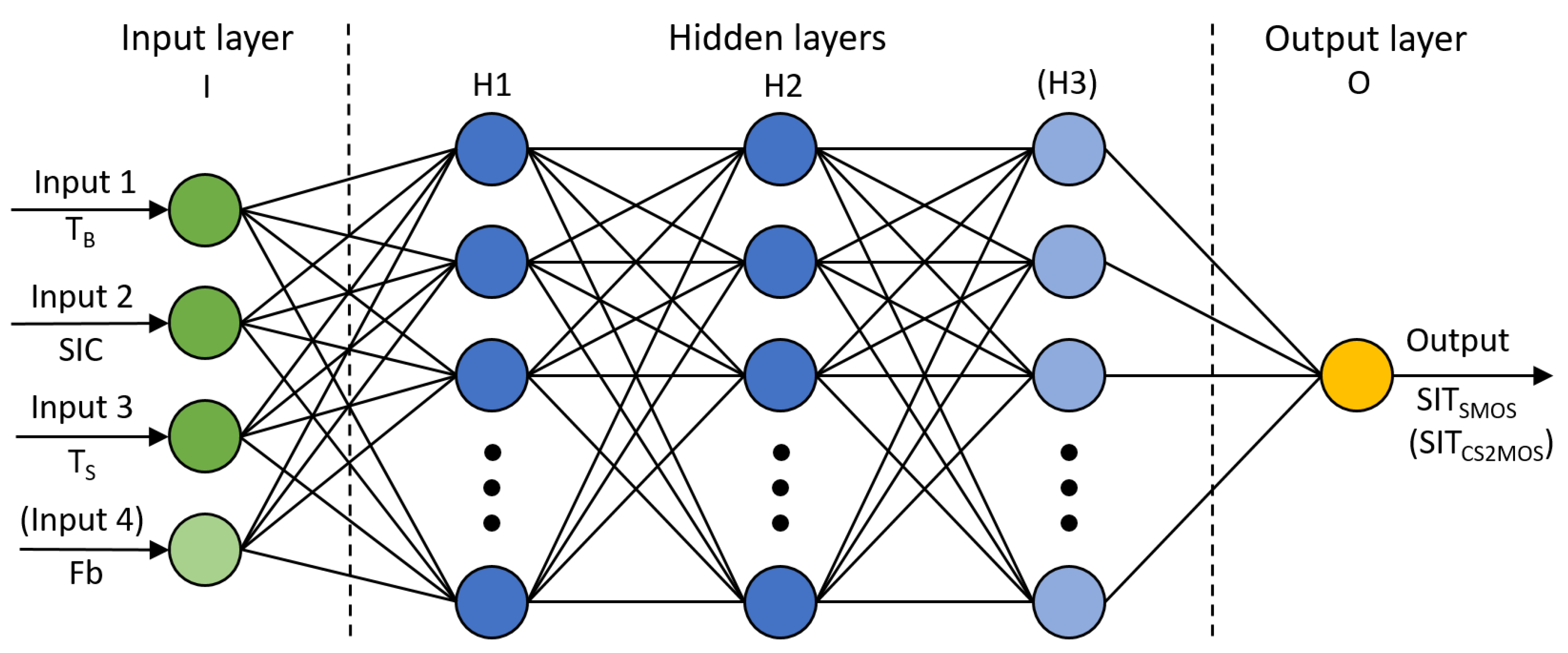
2.3. Implementation of the Regression NN

The goal of this study is to estimate Arctic and Antarctic SIT from the selected set of input features. Targeting continuous values of SIT based on the relationship between the input features represents a regression task. Linear regression models typically adjust a number of model parameters to a set of training data in an iterative process by minimizing a cost function, which eventually converges to an optimal fit. The Gradient Descent method is a common technique to find the optimum solution. It computes the local gradient with respect to the model parameters and a cost function, following the direction of descending gradient until reaching convergence [49]. In a first attempt, a simple regression model without hidden layers was selected, but the model did neither converge nor generalize well on the test set. This implied that the input features are not linearly separable, but rather non-linearly related.

Neural networks (NN) can manage complex regression tasks and they are more adequate than traditional approaches when dealing with non-linear relationships between the variables. In its basic structure, a NN consists of an input layer, an output layer, and interposed hidden layers, with each layer consisting of a number of neurons [50]. The observations for training are assigned to the input layer with the number of neurons being the number of input features. The output layer of a regression task has a single neuron that represents the retrieved continuous target parameter. At least one hidden layer between the input and output layer makes the model different from a simple regression framework by enabling the network to learn the relationships that are contained in the dataset. In this work, the networks were built as sequentially dense layers, i.e., each neuron of the previous layer is fully connected to all neurons of the following layer. The specific model set-up was adjusted during the training and Figure 3 illustrates the final network architecture for the thin and full-range model. Similar to the coefficients in a linear regression, each connection (lines) between neurons represents the weight of the output of the neuron in the previous layer. The output value Y of each neuron is determined by forward propagating the weighted sum of the inputs coming from the neurons i of the previous layer with the weights $\omega$ and an additive bias b

$$Y=f\left(\sum _i({\omega }_i\ast inpu{t}_i)+b\right)\mathrm{with}f\left(x\right)=max(0,x).$$

(1)

The activation function f of each hidden layer introduces the non-linearity between the input features and the target variable, without which the regression network would be entirely linear. ReLU (Rectified Linear Unit), representing the activation function defined above, is a commonly used function in regression tasks, and it has the advantage of being computationally efficient and it does not saturate for positive values [51]. The weights and biases of the neurons are updated according to the final error of the cost function via back-propagation. The number of hidden layers and neurons per layer can be increased to capture more feature interactions, depending on the complexity of the problem.

The specific model set-up was adjusted during the training. Adaptive Moment (Adam) estimation was selected as an optimizer [52]. Model parameters ($\omega$, b) were randomly initialized and a small learning rate of 0.001 was chosen to obtain smooth convergence. The entire feature set was split into a training set (80%) and a test set (20%). The training set was further split into a reduced training set (80%) and validation set (20%). The performance of the different models was quantified using the Mean Absolute Error (MAE) as a cost function, being defined as the average sum of absolute differences between ground truth and predicted SIT. The MAE value indicates the training and validation loss at each epoch of the training. The best performing model with the lowest MAE on the validation set was trained on the entire training set, and the resulting model was evaluated with the remaining test set.

Although preliminary results of an unconstrained network revealed low MAE for the known training data, the validation and training loss were not converging in the same way and the network resulted in different performances on training and validation set. Therefore, several constraints on the model hyperparameters were introduced to prevent the model from overfitting and overgeneralization. Regularization is used to prevent the model from overfitting by constraining the model complexity by keeping many model parameters close to zero (L2-regularization) or zero (L1-regularization) [53]. Hereby, the terms L1 and L2 refer to the norm, i.e., the L1-norm being the sum of the absolute values and the L2-norm being the square root of the squared distances. Weak L1 and L2 regularization was applied to all of the hidden layers in the regression network and the penalty terms were added to the cost function. Secondly, an Early Stopping technique prevents the model from overfitting by interrupting the training at the respective epoch, at which the validation loss reaches a minimum or stops to improve, i.e., no progress is obtained within a predefined number of epochs (patience interval). To train the model more efficiently, a relatively high number of neurons per layer (64) was selected in combination with Early Stopping regularization [54,55]. A sufficient amount of training data (∼350,000 samples for thin ice and 60,000 samples for the full-range SIT) allowed to set the batch size up to 1024 to restrain the amplitude of fluctuations of the validation loss and to reduce the total training time.

The two predictive neural networks were first trained in the Arctic. Subsequently, the network to estimate thin SIT was applied to the Arctic sea, and the network to estimate full-range SIT was applied to both Arctic and Antarctic seas. Prior to the training, the input features were processed to be treatable by the NN. Because the NN was trained using Gradient Descent method, it was required to scale and normalize the input features. This included normalization after filtering outliers to keep the variables within the reasonable ranges of values. Figure 4 shows the Kernel Density Estimation (KDE) charts of input features after defining their ranges of values, which were eventually used to train the thin and full-range SIT model, respectively.

An ocean-land mask was applied to all maps to exclude land areas. Additionally, an ocean-ice mask was applied to preserve data points over areas with a SIC > 15$\%$, being the minimum value for which the OSI-401-b SIC product is defined. T${}_B$ increases monotonically as a function of SIT and the interval of suitable values is defined between 100 K and 210 K, which is in agreement with the expected dynamic range of T${}_B$ when considering a SIT up to 0.6 m in Figure 2a (also under cold conditions). Only a small amount of larger values was filtered (<0.1$\%$ after applying the ocean-land and ocean-ice masks), which could be attributed to areas of possible land-sea contamination. For thin SIT prediction, a cutoff thickness (SIT${}_{max}$ = 0.6 m) was defined as the limit beyond which the sensitivity of T${}_B$ to SIT is assumed to be negligible. Regarding sea ice Fb, a threshold of 0.4 m is used as the upper limit for training the full-range model. As aforementioned, selective scaling and normalization of the input features were considered in the input layer of the network, according to the individual distribution of the input features.

Table 1. Summary statistics of the NN training set used to predict thin ice (top) and full-range thickness (bottom). The description includes the Mean, Standard Deviation (StDev), Minimum, and Maximum values of the observations.

Model	Input Feature	Mean	StDev	Min	Max
Thin ice	T${}_B$ [K]	166.8	21.3	100.0	209.7
	SIC [%]	80.4	20.1	18.8	100.0
	T${}_S$ [K]	264.1	5.1	236.4	281.4
	SIT${}_{SMOS}$ [m]	0.239	0.165	0.020	0.600
Full-range	T${}_B$ [K]	173.8	24.7	100.4	207.8
	SIC [%]	95.3	7.5	19.9	100.0
	T${}_S$ [K]	260.2	4.6	239.6	272.5
	Fb [m]	0.108	0.070	0.000	0.399
	SIT${}_{CS2SMOS}$ [m]	1.248	0.639	0.045	2.853

provides the summary statistics representing the final distribution and dispersion of the input features. After processing the data, a total of 348,009 and 63,330 instances were suitable for training the thin and full-range SIT models, respectively. Ground truth SIT${}_{SMOS}$ and SIT${}_{CS2SMOS}$ are only available from mid-October onwards and Fb data have a delayed delivery time of about one month. Therefore, the thin SIT model was trained with data from 15 October to 4 December, and the full-range SIT model was trained from 15 October to 21 November 2020, respectively. The thin and the full-range NN models were both trained based on Arctic T${}_B$ and ancillary data, and the model with the best fit was stored.

Unlike in simple regression or process-based models, the results of a NN cannot be extrapolated, since its input features are non-linearly related. NNs are based on the underlying statistics of the observations and a trained model can only be applied to new data in case the corresponding range of values is covered by that of the original training set. Thus, a reliable model prediction requires the variable space of the available training data to include the predicted data as an already learned subset. This can be assessed by comparing the training and prediction datasets regarding its variable ranges and the density of values. In case the values of the new dataset are located within the multi-dimensional convex hull of the original training dataset, the model output can be considered to be reliable. The convex hulls around the points clouds of all combinations of input features are presented in a two-dimensional sub-feature space in Figure 5, for the Arctic data (blue markers and black solid line) and for the Antarctic data (orange markers and red dashed line).

Both of the datasets are of the same quality and processed identically. The total number of valid observations for Arctic ice is higher because both the Fb and the T${}_B$ observations are less dense at higher latitudes, which reduces the amount of data for Antarctic sea ice. Regarding the distributions of T${}_B$, Fb and SIC, the ranges and densities of the observations in the Antarctic, are entirely covered within the hull of observations in the Arctic. Therefore, the full-range model, which was trained with Arctic data, is considered to be reliable for an application to the Antarctic data. It is important to mention that a small amount of T${}_S$ values in the Antarctic dataset is close to the sea ice melting point (>270 K). This is because the Antarctic summer had already started and the temperatures are high enough, so that sea ice located at lower latitudes begins to melt. The corresponding subset is not located within the convex hull of Arctic training data, which limits the reliability of the model predictions for these particular values.

3. Results

This section presents the results of the thin and full-range NN models. Section 3.1 describes the training procedure and indicates the model architectures of the best model fits. In Section 3.2, the corresponding models are applied to predict maps of Arctic thin SIT, and Arctic and Antarctic full-range SIT.

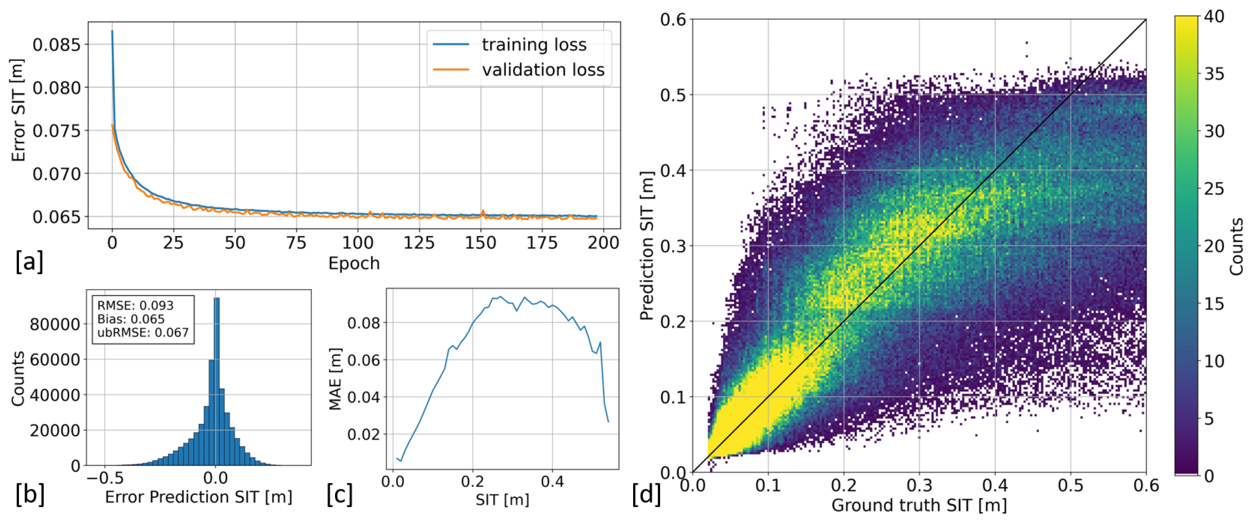
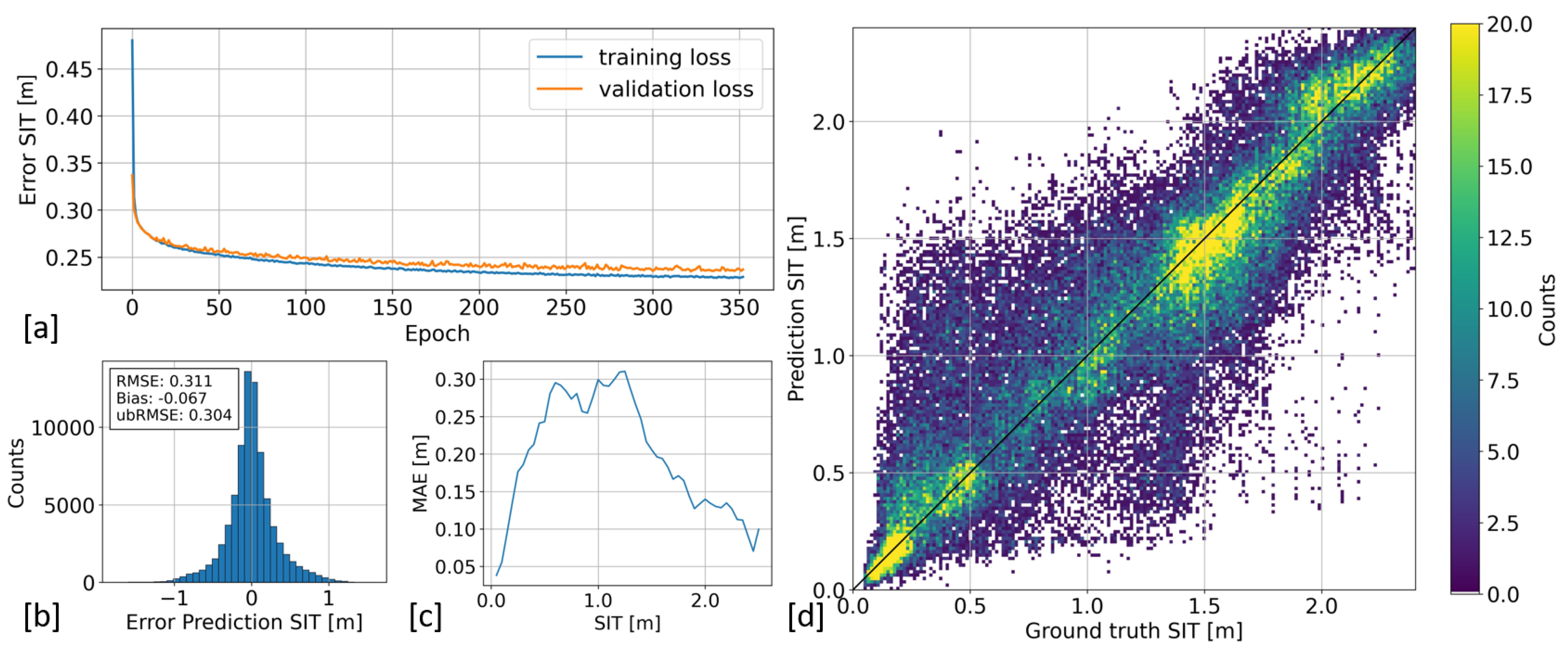
3.1. Training of the NN Models

During the training, various model architectures were adjusted and evaluated to minimize the generalization error (MAE) in order to obtain the model that fits the training data best. The hyperparameters were tuned to find a trade-off between training efficiency and convergence of the validation and training losses. The objective was to maintain the resemblance between the learning curves throughout the training to prevent overfitting and overgeneralization. Each model was trained with a maximum number of 1000 epochs, and both the training and validation losses were evaluated after each epoch, with a constant learning rate of 0.001. This rate turned out to be large enough to obtain a fast improvement of the learning curve at the beginning of the training (short burn-in phase) and small enough to lead to smooth convergence without bouncing around the optimum towards the end. In both NN (thin SIT and full-range SIT), the batch size, the number of hidden layers, and the patience interval of Early Stopping regularization were tuned, where the number of neurons per layer was kept constant to 64. An increase of the batch size up to a value of 1024 did not significantly influence the converging trend, but it considerably decreased the amplitude of the fluctuations in the validation loss and speeded up the training time. A higher number of hidden layers usually allows a network a fast build-up of sufficient complexity. In this case, more hidden layers (>3) led to a notable reduction of the training loss, whereas the validation loss was only slightly improving. This implied that, although the obtained model complexity apparently represented the reduced training set, it did not generalize well on the validation set. The validation loss fluctuated, but it showed a decreasing trend until it stagnated, when the model started to overfit the training data. Early Stopping with a patience interval eventually prevented the model from this overfitting. The fit was stopped after the validation loss did not show improvement anymore during the corresponding patience interval and the best fit was called-back and saved.

Table 2. A summary of training (top) and prediction (bottom) characteristics corresponding to the thin and full-range SIT models. The training characteristics comprise the model architecture and the adjusted hyperparameters for the optimal fit, including the total trained instances, the number of hidden layers and neurons per layer, batch size, patience interval for Early Stopping, and the number of trained epochs. Regarding the predictions, the obtained Mean Absolute Error (MAE) values are indicated for specific SIT ranges.

Training	Instances	Layers	Neurons	Batch Size	Patience	Epochs
Thin ice model	348,009	2	64	1024	30 epochs	198
Full-range model	63,330	3	64	1024	40 epochs	353
Prediction	Thin Ice Model		Full-Range Model
SIT range [m]	0–0.6		0–0.5	0.5–1.5	1.5–2.5	0–2.5
MAE [m]	0.065		0.160	0.275	0.149	0.237

provides a summary of the final architecture and the optimal training hyperparameters of the NNs and the SIT-range-specific MAE obtained from the prediction for the thin and full-range SIT models. The learning curves for the thin and full-range model are presented in Figure 6a and Figure 8a, respectively. Regarding both of the models, training and validation loss converged well, and no overfitting of the training data could be observed. Validation and training curves of the thin SIT model both match well throughout the training, whereas a small mismatch remained between those of the full-range SIT model towards the end of the training. The evaluation of the test set resulted in a final MAE of 0.065 m for the thin and 0.237 m for the full-range model, respectively.

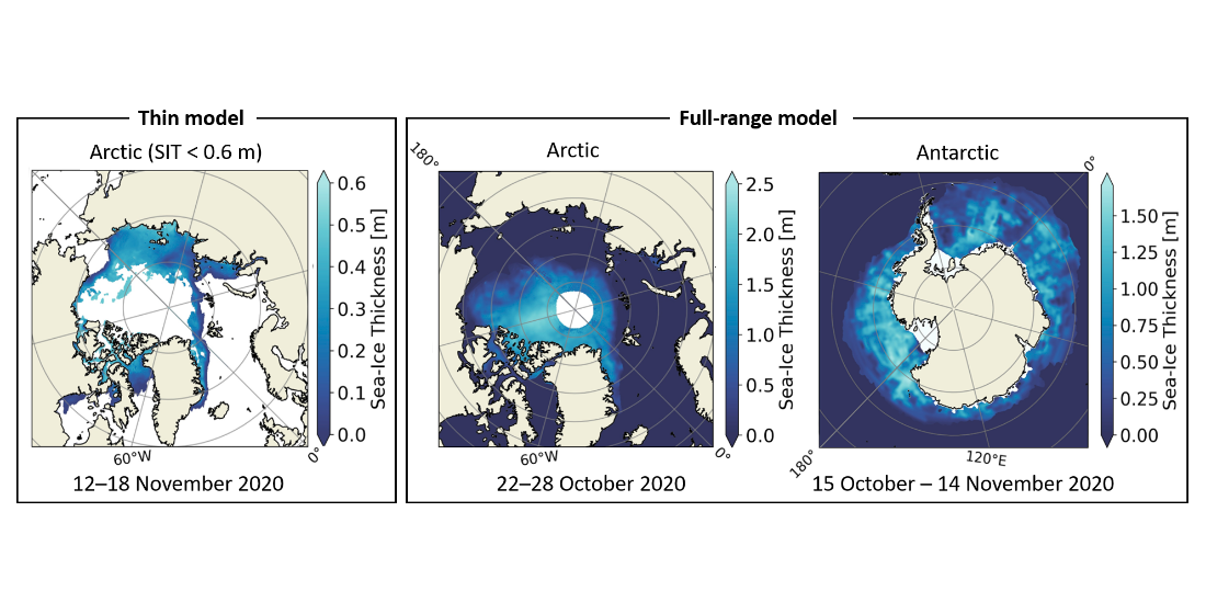
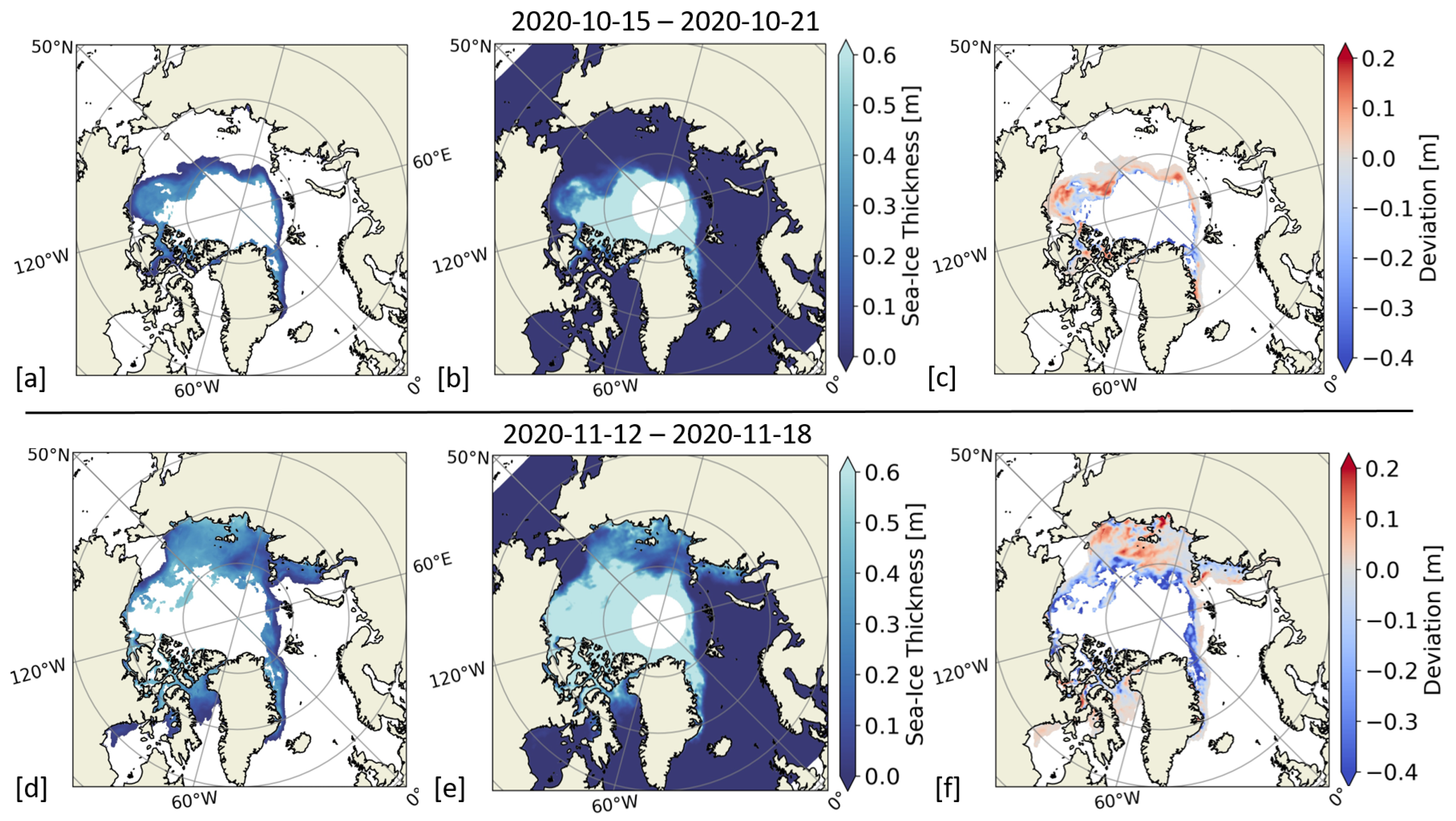
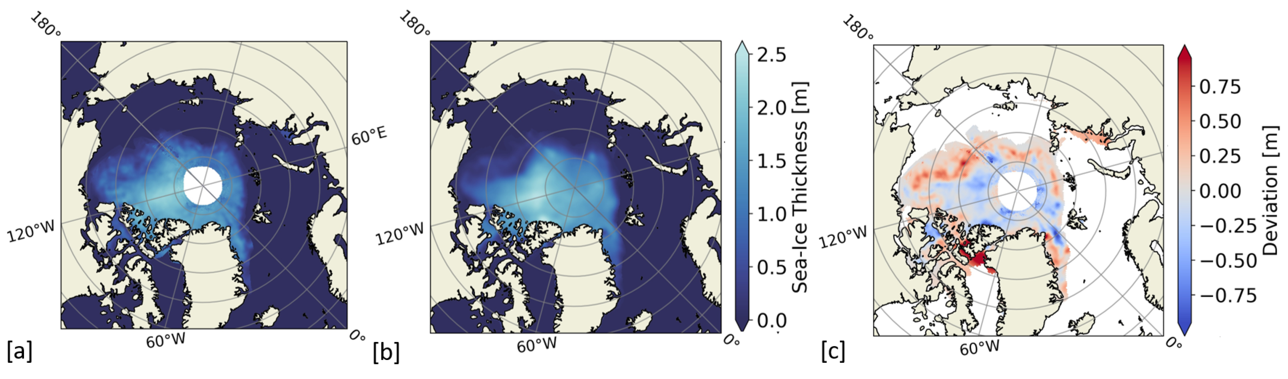
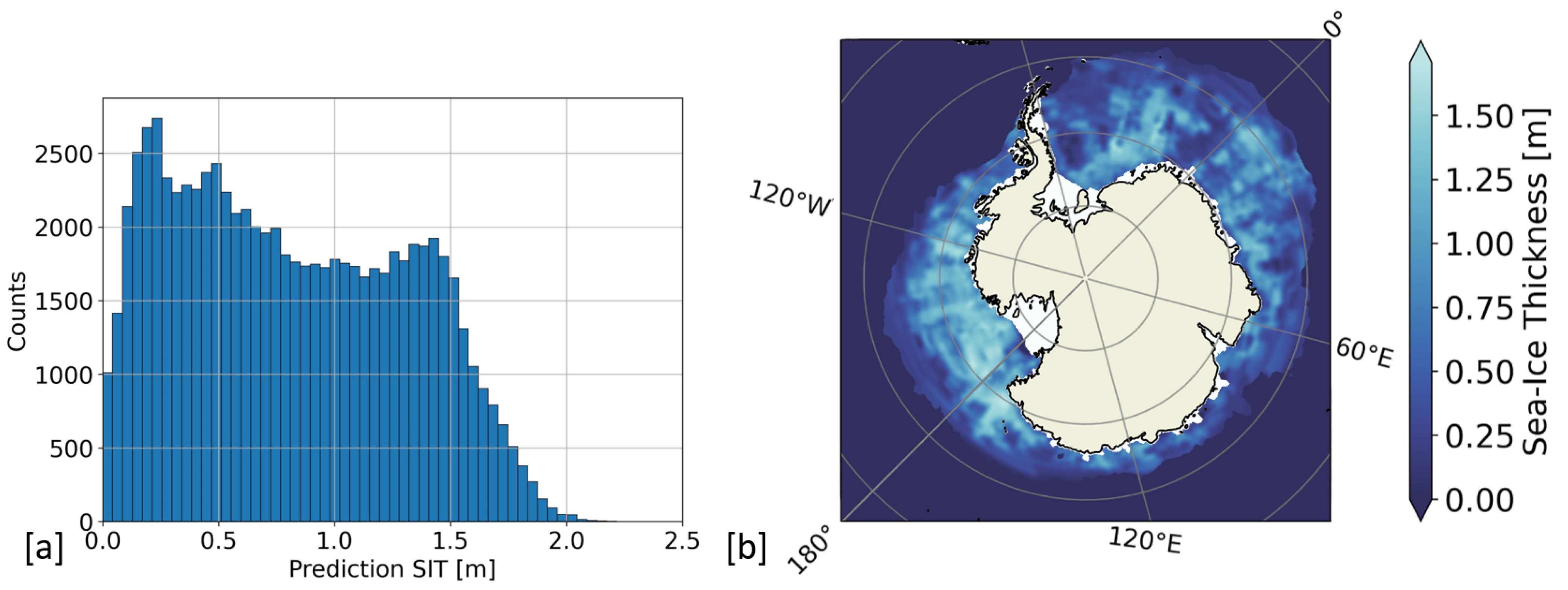
3.2. Prediction of Arctic and Antarctic SIT

The performance of the optimal fits was evaluated after applying the NN models to the unknown Arctic test set. The prediction error, the distribution of the MAE with SIT, and the relation between predicted and ground truth SIT are displayed in the Figure 6b–d for thin SIT. This model performs well with the error being widely unbiased up to a SIT of 0.4 m, but it underestimates the values for higher SIT. Predicted values deviate more from ground truth values with increasing SIT, until reaching a maximum error of around 9.5 cm at a SIT of approximately 30 cm. For predictions larger than 0.5 m, the MAE again shows lower values. This could be explained, because the model generally contains a small bias towards higher values and ground truth values beyond 0.6 m were filtered beforehand.

In Figure 7, two estimated weekly composite maps that are based on the thin SIT model are compared to the corresponding SIT${}_{SMOS}$ maps in the periods from 15–21 October and from 12–18 November 2020. In mid-October, sea ice mainly consisted of the remaining thick multi-year ice and regions of newly-formed thin ice were observed around the Beaufort Sea. In this period, only a small amount of under- and overestimated values are present. Positive deviations can be attributed to most-recently formed thin ice. Until mid-November, freeze-up had already advanced in the Arctic ocean, and thin sea ice below 0.6 m became more abundant. The increasing amount of newly-formed thin ice in the East Siberian Sea and the Laptev Sea, which is visible in the SIT${}_{SMOS}$ product, is in agreement with the values that were obtained from the NN model. In this period, the number of underestimated values increases as sea ice gets thicker. The deviations between the ground truth and the predicted values reveal that underestimated values are located around the 0.6 m threshold, where the model range is limited. They can be related to areas in the Beaufort Sea and the Greenland Sea, where sea ice started to thicken beyond the sensitivity range of T${}_B$ observations.

Figure 8b–d show the evaluation of the full-range SIT model. The model performs well for thin (<0.5 m) and for thicker ice (>1.5 m), in which a substantial amount of values is given. These include the individual sub-ranges, where T${}_B$ and altimetry observations are known to be more sensitive to SIT, and where uncertainties of the SIT${}_{SMOS}$ and the SIT${}_{CS2SMOS}$ products are expected to be lower. Most part of the elevated value of the total MAE (0.237 m) is made up by the high deviations of for SIT between 0.5 m and 1.5 m (∼0.25–0.30 m, with a MAE of 0.275 m in Table 2). This may occur due to the fact that, after summer melt and at the beginning of the freeze-up period, mainly thick multi-year ice remained together with thin newly-formed ice. Instead, only a few values of sea ice in the intermediate thickness range can be provided for model training during the observed period. Therefore, the intermediate range may be underrepresented in the resulting predictions. In addition, the ground truth values are based on T${}_B$ and altimetry observations using an optimal interpolation scheme. This may introduce some artifacts at intermediate SIT ranges, resulting in distortions in the training that cannot be adequately conceptualized by the NN model.

In Figure 9, the predicted weekly composite based on the full-range SIT model is compared to the corresponding SIT${}_{CS2SMOS}$ map in the period from 22–28 October 2020. The over- and underestimations may be due to the large footprint of the antenna, which smoothes out the observations, reducing the small-scale variability. Underestimations (indicated in blue) can be attributed to areas of more heterogeneous multi-year ice. Most of the overestimated values (indicated in red) are located in the Beaufort Sea and in areas with high contrasts between newly-formed thin ice and thicker ice. Hereby, predicted values are within the intermediate SIT range, in which the model performance is also less accurate. Highly overestimated values are located to the north of the Baffin Bay around North-Western Greenland. This anomaly may also be due to land-sea contamination or to most recently formed ice, which is not yet captured in the predicted weekly composite.

Figure 10 shows the predicted SIT map over the Antarctic sea from 15 October to 14 November 2020 (monthly composite), obtained after applying the full-range SIT model to Antarctic data. The massive ice shelves (e.g., Ronne and Ross) located in the Ross and Weddell sea were excluded from the predictions. It is important to note that a disseminated product of SIT at the Antarctic scale was at the time of the study not available for comparison. Therefore, the model cannot be validated in the same way as for the Arctic. SIT has an important impact on the melting trend of sea ice and it can be a good proxy of the upcoming SIE distribution. Antarctic SIE is already decreasing after having passed its annual sea ice maximum around mid-September. Thus, the spatial patterns of the distribution of SIT can be compared to those of future SIE, assuming that areas consisting of mainly thin ice are supposed to melt first. Because Antarctic sea ice melts and refreezes almost completely during a course of a year, it is mainly composed by thinner first-year ice. This is in agreement with the model predictions, which result in an average SIT of 0.67 m for the Antarctic, in comparison with 1.25 m obtained for the Arctic. Additionally, the maximum estimated SIT of 2 m in the Antarctic is lower than in the Arctic, where values up to 2.5 m were predicted.

4. Discussion

This work has presented the first results over polar areas using the FMPL-2 T${}_B$ observations of the FSSCat mission to predict SIT based on NN approaches. The thin SIT model performs well for sea ice up to ∼0.5 m. Above 0.5 m—where T${}_B$ is less sensitive to SIT—the values are notably underestimated, and the network is not capable of inferring SIT at higher range from the input feature interactions [5]. The retrieval algorithm of the corresponding SIT${}_{SMOS}$ product used as ground truth depends on the distribution of the physical temperature of sea ice and performs better for cold conditions [12]. This may contribute to the observed deviations between the model prediction and ground truth data for higher SIT. To extend the sensitivity range of the thin model, the input features are complemented with sea ice Fb observations from the Cryosat-2 mission to yield full-range SIT, using the SIT${}_{CS2SMOS}$ product as ground truth data. The full-range model performs well for values above 1.5 m and for thin SIT. However, between 0.5 m and 1.5 m, a gap of higher errors of magnitudes around 0.25 m to 0.3 m remains. The uncertainty of the merged SIT${}_{CS2SMOS}$ product is a combination of those of the original SIT maps that are derived from SMOS (SIT${}_{SMOS}$) and CryoSat-2 (SIT${}_{CS2}$) [21]. The observed errors of the model predictions in the intermediate SIT range between 0.5 m and 1.5 m are in agreement with those of the SIT${}_{SMOS}$ and SIT${}_{CS2}$ products, revealing high relative uncertainties between 25% and 75% in the same SIT range. Thus, the higher uncertainty of the SIT${}_{CS2SMOS}$ product at the mostly interpolated intermediate SIT range may affect the learning process during model training and it limits the prediction accuracy of the network at that particular range.

Instead of using the interpolated SIT${}_{CS2SMOS}$ product as a single target variable in the output layer of the network, more consistent predictions may be obtained by using SIT${}_{SMOS}$ and SIT${}_{CS2}$ data as two separate variables. The two predicted outputs could be interpolated a posteriori according to their individual error distributions. A conceivable solution to generally overcome the challenge of the remaining sensitivity gap—which is not covered by the altimetry measurements and the radiometry observations at L-band—will be to introduce another feature to the training set. Radiometry observations at P-band (∼500 MHz), as indicated in Figure 2b in Section ‘Data and Methods’, can complement the lack of sensitivity in the intermediate range. It can provide the necessary information content to the network to overcome the limitations of both the saturation of T${}_B$ for higher SIT and the predominantly high uncertainties of sea ice Fb corresponding to small SIT values.

Although ancillary data at higher resolution are added to reveal information of sea ice at smaller scale, the large radiometer footprint of ∼350 × 500 km${}^2$ smoothes out the observations and limits the detectable small-scale features of the SIT. Large-scale averaging overall reduces the standard deviation and the dynamic range of the T${}_B$ observations. Predictions of the full-range model are currently underestimated at areas of predominately thicker and more heterogeneous multi-year ice, where T${}_B$ observations at L-band are already saturated. Overestimated values are mostly located at the transitions between first-year and multi-year ice, and where high contrasts in SIT due to local variability are given. Therefore, the accuracy of SIT estimations while considering smaller scales is limited by the local heterogeneity of sea ice. The actual resolution of the FMPL-2 observations also depends on the orientation between the flight direction relative to the contrasts in surface structures of sea ice. Thus, it would be feasible to deploy a network of FMPL-2 like sensors in a constellation of CubeSats to shorten the revisit time.

The T${}_B$ discontinuities between land and sea ice close to coastal areas can lead to oscillations in the image reconstruction process (Gibbs phenomenon). T${}_B$ observations over land are sensitive to the soil moisture content, and values at L-band for circular-polarized near-nadir observations can range between around 175 K to 275 K [56]. This often results in higher T${}_B$ and an overestimation of SIT in land-sea contaminated areas. The accompanied artifacts can be corrected using a Gibbs algorithm similar to that which is used to derive T${}_B$ maps from SMOS data, but has not yet been implemented in the FMPL-2 T${}_B$ retrievals [57].

Regarding the range and density of values of Arctic training data and Antarctic prediction data, the application of the full-range model to predict Antarctic SIT was considered to be reliable during the study period. Because the Arctic and Antarctic regions represent different environments, accurate models require greater understanding on the temporal variability, sensitivity, and uncertainty contributions of the selected input features with respect to SIT estimations. So far, there is no validated product of Antarctic-wide SIT available using a process-based approach, mainly because these models require information on the physical properties, including snow cover. The signatures of radiometry measurements at L-band are sensitive to the intrinsic ice-physical properties, which change over the course of a year, and the conversion of satellite altimeter observations of Fb to SIT requires accurate knowledge of snow cover. Snow depth has been successfully estimated using approaches that are based on both emission models and NNs [29,30]. The uncertainty of SIT retrievals is largely determined by the uncertainty of current snow products, and the development of statistics-based models based on a appropriate set of features is promising, but it still remains challenging.

Because the seasons of freeze up and melting in the Northern Hemisphere are the opposite of those in the Southern Hemisphere and sea ice is located towards lower latitudes in the Antarctic, it largely consists of first-year ice throughout the year, which is generally shallower than in the Arctic. This is in agreement with the predictions of the full-range model, which result in an average SIT of 1.25 m for the Arctic and 0.67 m for the Antarctic, respectively. In the beginning of the Arctic freeze up, sea ice mainly consists of newly-formed thin ice and thick multi-year ice, agreeing with the range of thicker ice between 2 m and 2.5 m, which was only predicted over the Arctic. Unlike in the Arctic, parts of Antarctic sea ice surface temperatures reach the melting point during the observed period, which limits the reliability of the full-range model predictions for these particular values. In case the period of available training data was longer than the observed two months, the model training set should be periodically updated with new data, once any of the input features of the Antarctic prediction dataset reaches the limits of the training set.

5. Conclusions

Polar regions are environments with strong seasonal dynamics and spatial heterogeneity, which are difficult to be adequately addressed using process-based or simple regression models. This work has presented a new approach focusing on the retrieval of SIT maps based on predictive regression neural networks. Two independent models have been implemented and trained with Arctic data to yield maps of Arctic thin SIT and full-range SIT. Information regarding non-linearly related sea ice parameters is contained in hidden relationships between a selected number of observations. These relationships were considered in an additional number of hidden layers of a NN model. The model input features comprise of the FMPL-2 T${}_B$ observations that were provided by the FSSCat mission launched on 3 September 2020, which carries the FMPL-2 payload with the first GNSS-Reflectometer and L-band microwave radiometer on board a CubeSat, and ancillary data, including SIC and surface temperature maps. A thin SIT model was implemented using the SIT${}_{SMOS}$ product as ground truth data and targets SIT values up to 0.6 m, being limited by the sensitivity of L-band T${}_B$ observations. Adding complementary information of CryoSat-2 sea ice Fb data to the existing input features allowed us to extend the sensitivity range to values that are larger than those covered by the thin SIT model. This enabled implementing a second model yielding full-range SIT, which was evaluated using maps of the merged SIT${}_{CS2SMOS}$ product as ground truth data.

The input features were processed and both models were trained on Arctic data during early Arctic freeze up from 15 October to 4 December 2020. A number of hyperparameters was adjusted to prevent the models from data overfitting to obtain the optimal fit through the minimization of the MAE cost function. The thin ice model shows good performance with an overall MAE of 0.065 m and it generalizes well up to a SIT of 0.5 m, while underestimating for higher SIT values. The best fit of the full-range model results in a MAE of 0.237 m, and the predictions match well for thin ice and SIT above 1.5 m. Hereby, the main error contribution originates from predicted values in the intermediate SIT range. Major losses may be attributed to an existing sensitivity gap of the sensors or to the limited availability of sufficient values for training during the observed period.

The predictive models allowed for producing weekly composite maps of thin and full-range SIT at the Arctic scale. In a first attempt, the full-range model that was obtained from Arctic observations was also applied to Antarctic data to produce monthly composites of Antarctic SIT. It is important to note that a disseminated product of full-range SIT maps at Antarctic scale was not available for comparison during the observed period.

Neural networks have the advantage to be adaptive to new datasets and models are able to capture variable sea ice conditions and changing the relationships of the input variables when considering longer learning periods. Future tasks encompass the application of the methodology to additional data to better pinpoint limitations and evaluate model performance on regional scale. This work verified the success of the FSSCat mission and the potential of applying FMPL-2 T${}_B$ to estimate SIT over polar areas using data from a single CubeSat. Using a constellation of CubeSats of the same kind effectively increases the satellite revisit and the spatial resolution of T${}_B$ maps, and has the potential to improve model accuracy. These constellations would demonstrate a feasible moderate-cost alternative to complement large satellite mission or to substitute them during gaps of non-existent data, in order to guarantee the continuous monitoring of polar sea ice at both hemispheres.

References

1. NSIDC. Arctic Sea Ice at Minimum Extent for 2020. September 2020. Available online: https://nsidc.org/news/newsroom/arctic-sea-ice-minimum-extent-2020 (accessed on 13 January 2021).
2. Francis, J.A.; Vavrus, S.J. Evidence linking Arctic amplification to extreme weather in mid-latitudes. Geophys. Res. Lett. 2012, 39. [Google Scholar] [CrossRef]
3. Lindsay, R.; Schweiger, A. Arctic sea ice thickness loss determined using subsurface, aircraft, and satellite observations. Cryosphere 2015, 9, 269–283. [Google Scholar] [CrossRef] [Green Version]
4. Steffen, K. Considerations for microwave remote sensing of thin sea ice. Microw. Remote Sens. Sea Ice 1992, 68, 291–301. [Google Scholar] [CrossRef]
5. Naoki, K.; Ukita, J.; Nishio, F.; Nakayama, M.; Comiso, J.C.; Gasiewski, A. Thin sea ice thickness as inferred from passive microwave and in situ observations. J. Geophys. Res. Ocean. 2008, 113. [Google Scholar] [CrossRef] [Green Version]
6. Laxon, S.W.; Giles, K.A.; Ridout, A.L.; Wingham, D.J.; Willatt, R.; Cullen, R.; Kwok, R.; Schweiger, A.; Zhang, J.; Haas, C.; et al. CryoSat-2 estimates of Arctic sea ice thickness and volume. Geophys. Res. Lett. 2013, 40, 732–737. [Google Scholar] [CrossRef] [Green Version]
7. Guerreiro, K.; Fleury, S.; Zakharova, E.; Kouraev, A.; Rémy, F.; Maisongrande, P. Comparison of CryoSat-2 and ENVISAT radar freeboard over Arctic sea ice: Toward an improved Envisat freeboard retrieval. Cryosphere 2017, 11, 2059. [Google Scholar] [CrossRef] [Green Version]
8. Font, J.; Camps, A.; Borges, A.; Martín-Neira, M.; Boutin, J.; Reul, N.; Kerr, Y.H.; Hahne, A.; Mecklenburg, S. SMOS: The challenging sea surface salinity measurement from space. Proc. IEEE 2009, 98, 649–665. [Google Scholar] [CrossRef] [Green Version]
9. Kerr, Y.H.; Waldteufel, P.; Wigneron, J.P.; Delwart, S.; Cabot, F.; Boutin, J.; Escorihuela, M.J.; Font, J.; Reul, N.; Gruhier, C.; et al. The SMOS mission: New tool for monitoring key elements ofthe global water cycle. Proc. IEEE 2010, 98, 666–687. [Google Scholar] [CrossRef] [Green Version]
10. Kaleschke, L.; Tian-Kunze, X.; Maaß, N.; Mäkynen, M.; Drusch, M. Sea ice thickness retrieval from SMOS brightness temperatures during the Arctic freeze-up period. Geophys. Res. Lett. 2012, 39. [Google Scholar] [CrossRef]
11. Gupta, M.; Gabarro, C.; Turiel, A.; Portabella, M.; Martinez, J. On the retrieval of sea-ice thickness using SMOS polarization differences. J. Glaciol. 2019, 65, 481–493. [Google Scholar] [CrossRef] [Green Version]
12. Tian-Kunze, X.; Kaleschke, L.; Maaß, N.; Mäkynen, M.; Serra, N.; Drusch, M.; Krumpen, T. SMOS-derived thin sea ice thickness: Algorithm baseline, product specifications and initial verification. Cryosphere 2014, 8, 997–1018. [Google Scholar] [CrossRef] [Green Version]
13. Kaleschke, L.; Tian-Kunze, X.; Maaß, N.; Beitsch, A.; Wernecke, A.; Miernecki, M.; Müller, G.; Fock, B.H.; Gierisch, A.M.; Schlünzen, K.H.; et al. SMOS sea ice product: Operational application and validation in the Barents Sea marginal ice zone. Remote Sens. Environ. 2016, 180, 264–273. [Google Scholar] [CrossRef]
14. Huntemann, M.; Heygster, G.; Kaleschke, L.; Krumpen, T.; Mäkynen, M.; Drusch, M. Empirical sea ice thickness retrieval during the freeze up period from SMOS high incident angle observations. Cryosphere 2014, 8, 439–451. [Google Scholar] [CrossRef] [Green Version]
15. Paţilea, C.; Heygster, G.; Huntemann, M.; Spreen, G. Combined SMAP-SMOS thin sea ice thickness retrieval. Cryosphere 2019, 13, 675–691. [Google Scholar] [CrossRef] [Green Version]
16. Wingham, D.; Francis, C.; Baker, S.; Bouzinac, C.; Brockley, D.; Cullen, R.; de Chateau-Thierry, P.; Laxon, S.; Mallow, U.; Mavrocordatos, C.; et al. CryoSat: A mission to determine the fluctuations in Earth’s land and marine ice fields. Adv. Space Res. 2006, 37, 841–871. [Google Scholar] [CrossRef]
17. Ricker, R.; Hendricks, S.; Helm, V.; Skourup, H.; Davidson, M. Sensitivity of CryoSat-2 Arctic sea-ice freeboard and thickness on radar-waveform interpretation. Cryosphere 2014, 8, 1607–1622. [Google Scholar] [CrossRef] [Green Version]
18. Kurtz, N.; Harbeck, J. CryoSat-2 Level 4 Sea Ice Elevation. In Freeboard, and Thickness, Version 1; NASA National Snow and Ice Data Center Distributed Active Archive Center: Boulder, CO, USA, 2017. [Google Scholar]
19. Tilling, R.L.; Ridout, A.; Shepherd, A. Estimating Arctic sea ice thickness and volume using CryoSat-2 radar altimeter data. Adv. Space Res. 2018, 62, 1203–1225. [Google Scholar] [CrossRef]
20. Kaleschke, L.; Tian-Kunze, X.; Maaß, N.; Ricker, R.; Hendricks, S.; Drusch, M. Improved retrieval of sea ice thickness from SMOS and CryoSat-2. In Proceedings of the 2015 IEEE International Geoscience and Remote Sensing Symposium (IGARSS), Milan, Italy, 26–31 July 2015; pp. 5232–5235. [Google Scholar]
21. Ricker, R.; Hendricks, S.; Kaleschke, L.; Tian-Kunze, X.; King, J.; Haas, C. A weekly Arctic sea-ice thickness data record from merged CryoSat-2 and SMOS satellite data. Cryosphere 2017, 11, 1607–1623. [Google Scholar] [CrossRef] [Green Version]
22. Lee, S.; Im, J.; Kim, J.; Kim, M.; Shin, M.; Kim, H.C.; Quackenbush, L.J. Arctic sea ice thickness estimation from CryoSat-2 satellite data using machine learning-based lead detection. Remote Sens. 2016, 8, 698. [Google Scholar] [CrossRef] [Green Version]
23. Shen, X.Y.; Zhang, J.; Meng, J.M.; Ke, C.Q. Sea ice type classification based on random forest machine learning with Cryosat-2 altimeter data. In Proceedings of the 2017 International Workshop on Remote Sensing with Intelligent Processing (RSIP), Shanghai, China, 18–21 May 2017; pp. 1–5. [Google Scholar]
24. Herbert, C.; Camps, A.; Wellmann, F.; Vall-Llossera, M. Bayesian unsupervised machine learning approach to segment Arctic sea ice using SMOS data. Geophys. Res. Lett. 2021, 48. [Google Scholar] [CrossRef]
25. Belchansky, G.; Douglas, D.C.; Platonov, N.G. Fluctuating Arctic sea ice thickness changes estimated by an in situ learned and empirically forced neural network model. J. Clim. 2008, 21, 716–729. [Google Scholar] [CrossRef]
26. Lin, H.; Yang, L. A hybrid neural network model for sea ice thickness forecasting. In Proceedings of the 2012 8th International Conference on Natural Computation, Chongqing, China, 29–31 May 2012; pp. 358–361. [Google Scholar]
27. Chi, J.; Kim, H.C. Prediction of arctic sea ice concentration using a fully data driven deep neural network. Remote Sens. 2017, 9, 1305. [Google Scholar]
28. Tedesco, M.; Pulliainen, J.; Takala, M.; Hallikainen, M.; Pampaloni, P. Artificial neural network-based techniques for the retrieval of SWE and snow depth from SSM/I data. Remote Sens. Environ. 2004, 90, 76–85. [Google Scholar] [CrossRef]
29. Maaß, N.; Kaleschke, L.; Tian-Kunze, X.; Drusch, M. Snow thickness retrieval over thick Arctic sea ice using SMOS satellite data. Cryosphere 2013, 7, 1971–1989. [Google Scholar] [CrossRef] [Green Version]
30. Liu, J.; Zhang, Y.; Cheng, X.; Hu, Y. Retrieval of snow depth over arctic sea ice using a deep neural network. Remote Sens. 2019, 11, 2864. [Google Scholar] [CrossRef] [Green Version]
31. Braakmann-Folgmann, A.; Donlon, C. Estimating snow depth on Arctic sea ice using satellite microwave radiometry and a neural network. Cryosphere 2019, 13, 2421–2438. [Google Scholar] [CrossRef] [Green Version]
32. Kilic, L.; Prigent, C.; Aires, F.; Boutin, J.; Heygster, G.; Tonboe, R.T.; Roquet, H.; Jimenez, C.; Donlon, C. Expected performances of the Copernicus Imaging Microwave Radiometer (CIMR) for an all-weather and high spatial resolution estimation of ocean and sea ice parameters. J. Geophys. Res. Ocean. 2018, 123, 7564–7580. [Google Scholar] [CrossRef] [Green Version]
33. Donlon, C. Copernicus Imaging Microwave Radiometer (CIMR) Mission Requirements Document, Version 2.0; European Space Agency, ESTEC: Noordwijk, The Netherlands, 2019. [Google Scholar]
34. Kulu, E. World’s Largest Database of Nanosatellites, Over 2700 Nanosats and CubeSats (2014–2020). Available online: https://www.nanosats.eu/ (accessed on 30 December 2020).
35. Camps, A. Nanosatellites and Applications to Commercial and Scientific Missions. In Satellites and Innovative Technology; IntechOpen: London, UK, 2019. [Google Scholar]
36. Kramer, H. Flock 1 Imaging Constellation Built by Planet Labs Inc. Available online: https://earth.esa.int/web/eoportal/satellite-missions/f/flock-1 (accessed on 21 January 2021).
37. SpaceNews. Spire Adding Cross Links to Cubesat Constellation. September 2020. Available online: https://spacenews.com/spire-adding-cross-links-to-cubesat-constellation/ (accessed on 21 January 2021).
38. Munoz-Martin, J.F.; Capon, L.F.; Ruiz-de Azua, J.A.; Camps, A. The Flexible Microwave Payload-2: A SDR-Based GNSS-Reflectometer and L-Band Radiometer for CubeSats. IEEE J. Sel. Top. Appl. Earth Obs. Remote Sens. 2020, 13, 1298–1311. [Google Scholar] [CrossRef]
39. Munoz-Martin, J.F.; Fernandez, L.; Perez, A.; Ruiz-de Azua, J.A.; Park, H.; Camps, A.; Domínguez, B.C.; Pastena, M. In-Orbit Validation of the FMPL-2 Instrument—The GNSS-R and L-Band Microwave Radiometer Payload of the FSSCat Mission. Remote Sens. 2021, 13, 121. [Google Scholar] [CrossRef]
40. Camps, A.; Golkar, A.; Gutierrez, A.; de Azua, J.R.; Munoz-Martin, J.F.; Fernandez, L.; Diez, C.; Aguilella, A.; Briatore, S.; Akhtyamov, R.; et al. FSSCAT, the 2017 Copernicus Masters’ “ESA Sentinel Small Satellite Challenge” Winner: A Federated Polar and Soil Moisture Tandem Mission Based on 6U Cubesats. In Proceedings of the IGARSS 2018-2018 IEEE International Geoscience and Remote Sensing Symposium, Valencia, Spain, 22–27 July 2018; pp. 8285–8287. [Google Scholar]
41. Bentley, J.L. Multidimensional binary search trees used for associative searching. Commun. ACM 1975, 18, 509–517. [Google Scholar] [CrossRef]
42. Comiso, J.C.; Parkinson, C.L.; Markus, T.; Cavalieri, D.J.; Gersten, R. Current State of Sea Ice Cover. Available online: https://earth.gsfc.nasa.gov/cryo/data/current-state-sea-ice-cover (accessed on 30 December 2020).
43. Comiso, J.C.; Cavalieri, D.J.; Parkinson, C.L.; Gloersen, P. Passive microwave algorithms for sea ice concentration: A comparison of two techniques. Remote Sens. Environ. 1997, 60, 357–384. [Google Scholar] [CrossRef]
44. Ulaby, F.T.; Moore, R.; Fung, A. Microwave Remote Sensing: Active and Passive. Volume 3-From Theory to Applications; Artech House Inc.: Dedham, MA, USA, 1986. [Google Scholar]
45. Menashi, J.D.; St. Germain, K.M.; Swift, C.T.; Comiso, J.C.; Lohanick, A.W. Low-frequency passive-microwave observations of sea ice in the Weddell Sea. J. Geophys. Res. Ocean. 1993, 98, 22569–22577. [Google Scholar] [CrossRef]
46. Zeng, X.; Beljaars, A. A prognostic scheme of sea surface skin temperature for modeling and data assimilation. Geophys. Res. Lett. 2005, 32. [Google Scholar] [CrossRef] [Green Version]
47. Warren, S.G.; Rigor, I.G.; Untersteiner, N.; Radionov, V.F.; Bryazgin, N.N.; Aleksandrov, Y.I.; Colony, R. Snow depth on Arctic sea ice. J. Clim. 1999, 12, 1814–1829. [Google Scholar] [CrossRef]
48. No, D. CRYOSAT Ground Segment. 2009. Available online: https://earth.esa.int/documents/10174/125273/CryoSat-L2-Products-Format-Specification-v4.5.pdf (accessed on 17 March 2021).
49. Chong, E.K.; Zak, S.H. An Introduction to Optimization; John Wiley & Sons: Hoboken, NJ, USA, 2004. [Google Scholar]
50. LeCun, Y.; Bengio, Y.; Hinton, G. Deep learning. Nature 2015, 521, 436–444. [Google Scholar] [CrossRef]
51. Géron, A. Hands-on Machine Learning with Scikit-Learn, Keras, and TensorFlow: Concepts, Tools, and Techniques to Build Intelligent Systems; O’Reilly Media: Newton, MA, USA, 2019. [Google Scholar]
52. Kingma, D.P.; Ba, J. Adam: A method for stochastic optimization. arXiv 2014, arXiv:1412.6980. [Google Scholar]
53. Kuhn, M.; Johnson, K. Applied Predictive Modeling; Springer: New York, NY, USA, 2013; Volume 26. [Google Scholar]
54. Jaderberg, M.; Dalibard, V.; Osindero, S.; Czarnecki, W.M.; Donahue, J.; Razavi, A.; Vinyals, O.; Green, T.; Dunning, I.; Simonyan, K.; et al. Population based training of neural networks. arXiv 2017, arXiv:1711.09846. [Google Scholar]
55. Smith, L.N. A disciplined approach to neural network hyper-parameters: Part 1—Learning rate, batch size, momentum, and weight decay. arXiv 2018, arXiv:1803.09820. [Google Scholar]
56. De Roo, R.D.; England, A.W.; Munn, J. Circular polarization for L-band radiometric soil moisture retrieval. In Proceedings of the 2004 IEEE Aerospace Conference Proceedings (IEEE Cat. No. 04TH8720), Big Sky, MT, USA, 6–13 March 2004; Volume 2, pp. 1015–1023. [Google Scholar]
57. Oliva, R.; Martín-Neira, M.; Corbella, I.; Closa, J.; Zurita, A.; Cabot, F.; Khazaal, A.; Richaume, P.; Kainulainen, J.; Barbosa, J.; et al. SMOS Third Mission Reprocessing after 10 Years in Orbit. Remote Sens. 2020, 12, 1645. [Google Scholar] [CrossRef]
Figure 1. Maps of the input features for 11 November 2020, comprising (a) FMPL-2 T B , (b) OSI-SAF OSI-401-b SIC, (c) ECMWF Skin temperature, and (d) CryoSat-2 sea ice Fb (weekly composite).
Remotesensing 13 01366 g001
Figure 2. Relationship between T B and sea ice thickness (SIT) as a function of T P h of sea ice and sea ice types. Estimations are obtained using a radiative transfer model based on empirically determined values for salinity, density, and surface roughness. The curves represent circular-polarized emissions obtained with a nadir-pointing antenna at two frequencies, (a) at L-band (1.4 GHz, similar to T B observations of the FMPL-2 radiometer) and (b) at P-band (500 MHz).
Remotesensing 13 01366 g002
Figure 3. Principle architecture of the implemented neural networks (NN) consisting of a multiple-input normalization layer adapted to the number of input features, i.e., T B , SIC, T S , and Fb (in case of the full-range model), a number of non-linear hidden layers with a number of neurons per layer, and a linear single-output layer yielding continuous values of SIT. The final network architecture contains 2 or 3 hidden layers with 64 neurons per layer regarding the thin or full-range model, respectively.
Remotesensing 13 01366 g003
Figure 4. Kernel Density Estimation (KDE) charts of the NN training sets used to train the thin sea ice (a) and the full-range model (b), including the marginal probability density functions of the filtered datasets. The thin model is based on T B , SIC, T S and ground truth thin SIT derived from Soil Moisture and Ocean Salinity (SMOS). The full-range SIT model is based on T B , SIC, T S , Fb, and ground truth SIT derived from CryoSat-2 and SMOS.
Remotesensing 13 01366 g004
Figure 5. Convex hulls around the point clouds in two-dimensional sub-feature space of Arctic data (black solid line around blue markers), and Antarctic data (red dashed line around yellow markers) (Feature pairs: (a) T B –T S , (b) T B –SIC, (c) T B –Fb, (d) Fb–SIC, (e) Fb–T S , and (f) SIC–T S ). The application of the full-range model to Antarctic data is considered to be reliable, since most of its values are located within the convex hull and at denser areas of Arctic training data.
Remotesensing 13 01366 g005
Figure 6. Evaluation of training and prediction of the thin SIT model. (a) Validation and training error determined after each epoch; early stopping occurred at 198 iterations and the model resulted in a MAE of 0.065 m; (b) prediction error after application of the model to the entire Arctic dataset; (c) distribution of the MAE with SIT; and, (d) relation between predicted and ground truth SIT S M O S .
Remotesensing 13 01366 g006
Figure 7. Weekly maps of predicted thin SIT (a,d), the corresponding ground truth SIT S M O S (b,e), and deviations with respect to SIT S M O S (c,f), over the Arctic sea from 15–21 October and from 12–18 November 2020, respectively. Areas with SIT S M O S > 0.6 m were filtered in the predictions.
Remotesensing 13 01366 g007
Figure 8. Evaluation of training and prediction of the full-range SIT model. (a) Validation and training error determined after each epoch converge close to each other; early stopping occurred around 353 iterations and the model resulted in a MAE of 0.237 m; (b) prediction error after application of the model to the entire Arctic dataset; (c) distribution of the MAE with SIT; (d) relation between predicted and ground truth SIT C S 2 S M O S ; Good generalization is obtained for thin ice (SIT < 0.5 m) and thicker ice (SIT > 1.5 m).
Remotesensing 13 01366 g008
Figure 9. Comparison between the weekly composites of predicted Arctic full-range SIT maps (a) and the corresponding ground truth SIT C S 2 S M O S product (b), including their deviations (c), from 22–28 October 2020.
Remotesensing 13 01366 g009
Figure 10. Application of the Arctic full-range SIT model to Antarctic data. (a) Distribution of the predicted SIT values; (b) Monthly composite of Antarctic full-range SIT from 15 October to 14 November 2020.
Remotesensing 13 01366 g010