Abstract
In this paper, land subsidence susceptibility was assessed for Shahryar County in Iran using the adaptive neuro-fuzzy inference system (ANFIS) machine learning algorithm. Another aim of the present paper was to assess if ensembles of ANFIS with two meta-heuristic algorithms (imperialist competitive algorithm (ICA) and gray wolf optimization (GWO)) would yield a better prediction performance. A remote sensing synthetic aperture radar (SAR) dataset from 2019 to 2020 and the persistent-scatterer SAR interferometry (PS-InSAR) technique were used to obtain a land subsidence inventory of the study area and use it for training and testing models. Resulting PS points were divided into two parts of 70% and 30% for training and testing the models, respectively. For susceptibility analysis, eleven conditioning factors were taken into account: the altitude, slope, aspect, plan curvature, profile curvature, topographic wetness index (TWI), distance to stream, distance to road, stream density, groundwater drawdown, and land use/land cover (LULC). A frequency ratio (FR) was applied to assess the correlation of factors to subsidence occurrence. The prediction power of the models and their generated land subsidence susceptibility maps (LSSMs) were validated using the root mean square error (RMSE) value and area under curve of receiver operating characteristic (AUC-ROC) analysis. The ROC results showed that ANFIS-ICA had the best accuracy (0.932) among the models (ANFIS-GWO (0.926), ANFIS (0.908)). The results of this work showed that optimizing ANFIS with meta-heuristics considerably improves LSSM accuracy although ANFIS alone had an acceptable result.
1. Introduction
Land subsidence (LS) is one of the most challenging catastrophic geohazards due to its potential consequences, including damage to infrastructures, power lines, and buildings, causing sinkholes, floods in coastal areas, and soil degradation [1,2,3]. Land subsidence is a gradual and slow deformation or sudden collapse of the Earth’s surface, which is caused by numerous natural and human-induced factors [4,5,6,7]. The ground subsiding movement can be the result of natural causes such as floods, ground lithology, dissolution of carbonated rocks (e.g., limestone), sediment compaction, and tectonic motions of faults [8,9,10,11]. Further, anthropogenic activities that alleviate these geological factors, including underground excavations (e.g., mining and tunneling), underground resource withdrawal (gas or oil), overloading of the land surface through road construction and extending the built environment [12,13,14], and most importantly, over-exploitation of underground aquifers [15,16,17].
In the last few decades, the land subsidence phenomenon has widely increased in Iran [18,19,20], and therefore, growing research interest has focused on studying this geological problem [2,13,17,21,22,23]. One of the most important causes of the LS in Iran with an arid and semi-arid environment is the excessive groundwater extraction for agricultural usage [13,24]. Therefore, modeling factors affecting land subsidence and land subsidence susceptibility mapping (LSSM) is vital for the environment, safety, economy, and human well-being.
Remote sensing (RS) and geographic information system (GIS) data and tools have been helpful in land subsidence susceptibility studies in terms of acquiring fine resolution data and analyzing various factors affecting this phenomenon [10,11,25]. Many statistical and probabilistic approaches have been applied in the literature to provide susceptibility maps and monitor subsidence. These methods include the frequency ratio (FR) [26], weight of evidence (WOE) [27], logistic regression (LR) [28], evidential belief function (EBF) models [11], artificial neural networks (ANNs) [29,30], analytical hierarchy processes (AHP) [31,32], multi-criteria decision making (MCDM) models [22], as well as fuzzy logic (FL) [27,30] and adaptive neuro-fuzzy inference systems (ANFIS) [33].
However, these methods are mainly based on human assumptions and need expert knowledge. Recently, GIS-based machine learning algorithms (MLAs) have become a favorite in modeling and analyzing environmental hazards, especially LS. They can cope with data peculiarities, reveal complex relationships between data, and produce high accuracy and close-to-real world results [10,23]. Lee and Park [12] conducted a comparative investigation between the decision tree (DT) algorithm and FR model in estimation of LS and its causing factors. Abdollahi et al. [34] applied a support vector machine (SVM) to predict LSS using water table drawdown and other influential factors. Taravatrooy et al. [35] used a hybrid clustering method based on k-means, genetic optimization, and several soft computing algorithms to examine subsided zones. Tien Bui et al. [10] compared four MLAs (Bayesian logistic regression (BLR), SVM, logistic model tree (LMT), and alternate decision tree (ADT)) in assessing LSS near abandoned mining areas in South Korea. In a study in Kerman, Iran, the random forest (RF) algorithm showed superior capability in LSS mapping [36]. Ebrahimy et al. [23] performed a comparative study using three tree-based MLAs, a boosted regression tree (BRT), RF, and classification and regression tree (CART), for studying land susceptibility in Tasuj plane, Iran. Evaluation results revealed that BRT had the best performance. In another study by Rahmati et al. [37], four tree-based MLAs, a rule-based decision tree (RDT), RF, CART, and BRT, were compared for generating LS hazard maps in Hamedan Province, Iran. The results indicated that RF had the best accuracy amongst the employed methods.
Despite the better performance and accuracy of MLAs, all the above-mentioned approaches are dependent on the availability and precision of the subsidence inventory data, which is a serious challenge in developing countries [2,11,37]. On the other hand, interferometric synthetic aperture radar (InSAR) has been utilized in land displacement measurement and demonstrated promising results with millimetric precision [38,39]. SAR is satellite data so there is no need for time-consuming field survey data acquisition; therefore, it is superior to other approaches such as leveling data and is denser than ground positioning system (GPS) station data. Furthermore, radar data are functional in all-time all-weather conditions, making this a cost-efficient method to obtain land subsidence measurements. Recently, InSAR methods were employed in LSS studies as reliable input data along with other data to achieve finer accuracies [6,40]. In this paper, we used the PS-InSAR method to obtain land subsidence inventory data and utilize them among other subsidence triggering factors for land subsidence susceptibility mapping in the study area. As a novel methodology in LSSM, we used ANFIS optimized with two meta-heuristic algorithms: (1) imperialist competitive algorithm (ICA) and (2) gray wolf optimization (GWO). ANFIS uses hybrid learning of ANN in adjusting its membership functions (MF) with output data [41,42]. Further, by taking advantage of meta-heuristic algorithms, the weight parameters of MFs were optimized. The results of the method were compared using the statistical approach of the root mean square error (RMSE) value. Furthermore, the accuracy of LSSMs was evaluated by the area under the receiver operating characteristic (ROC) curve.
2. Materials and Methods
The methodology applied in this research (summarized in Figure 1) is to generate an updated land subsidence inventory through the PSInSAR technique using a Sentinel-1 SAR dataset spanning the period from 2019 to 2020. Moreover, the aim of this paper is to develop and use an ensemble of ANFIS and meta-heuristic algorithms in modeling land subsidence susceptibility. The main steps of the study are as follows. First, a spatial database was created using generated land subsidence inventory and the layers of the conditioning factors. In the second step, PS-InSAR-derived subsidence inventory data were divided into training (70%) and testing (30%) data. Next, MF parameters were optimized in ANFIS using ICA and GWO meta-heuristic algorithms, and then LSSMs were produced using ANFIS, ANFIS-ICA, and ANFIS-GWO individually. Finally, the produced land susceptibility maps were compared and evaluated using the area under the ROC curves.
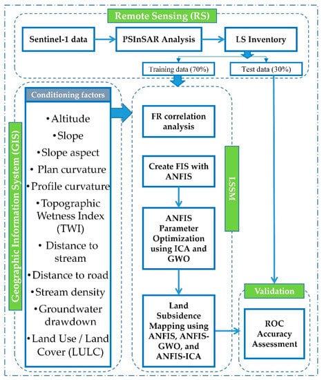
Figure 1.
Flowchart of the overall methodology.
2.1. Study Area
The region of interest in this paper is Shahryar, the central city of Shahryar County within 35°35′ to 35°42′ latitudes and 50°59′ to 51°6′ longitudes (Figure 2), with the elevation ranging from 1081 to 1222 m. This county is located west of Tehran, the capital of Iran. In recent years, there has been an increase in population migration to cities near Tehran, including Shahryar, for better jobs and income. According to Iran census data in 2016, the county is the 12th largest in the country with a population of more than 700,000 people. This has become a serious problem in urban environment management and food production. Shahryar County is known for its green and beautiful landscape and the major income of the people in the area originates from gardening and agriculture. Owing to population increase, the demand for food has grown dramatically. Therefore, more illegal wells are dug. As a result, the county has suffered from severe land subsidence (250 to 310 mm/year) due to exhaustion of underground water aquifers and water table dropdown.
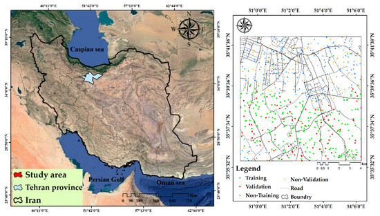
Figure 2.
The location of the study area along with the extracted land subsidence inventory.
The region of interest in this paper is Shahryar, the central city of Shahryar County within 35°35′ to 35°42′ latitudes and 50°59′ to 51°6′ longitudes (Figure 2), with the elevation ranging from 1081 to 1222 m. This county is located west of Tehran, the capital of Iran. In recent years, there has been an increase in population migration to cities near Tehran, including Shahryar, for better jobs and income. According to Iran census data in 2016, the county is the 12th largest in the country with a population of more than 700,000 people. This has become a serious problem in urban environment management and food production. Shahryar County is known for its green and beautiful landscape and the major income of the people in the area originates from gardening and agriculture. Owing to population increase, the demand for food has grown dramatically. Therefore, more illegal wells are dug. As a result, the county has suffered from severe land subsidence (250 to 310 mm/year) due to exhaustion of underground water aquifers and water table dropdown.
2.2. Date Used
As outlined earlier, the methodology has two main parts. One is the procedure of generating a land subsidence inventory using the PS-InSAR technique, which needs a satellite SAR dataset. The other is the conditioning factors that are taken into consideration for hazard modeling. In the following section, the process of acquiring and preparing these datasets is discussed.
2.2.1. SAR Data
To generate a land subsidence inventory in order to acquire the training and testing data necessary for LSSM, sentinel-1A single look complex (SLC) SAR data provided by European Space Agency (ESA) were used. In total, 31 SAR images were obtained from January 2019 to January 2020 in ascending track with dual polarization (vertical–vertical and vertical–horizontal) (Table 1).

Table 1.
The details of the SAR data used.
2.2.2. Factors Affecting Land Subsidence
To date, there is no single guideline unanimously applied for selecting subsidence-affecting factors. However, based on the literature of LSSM studies carried out in Iran [13,23,33,37], data that were directly and indirectly related to the subsidence-inducing factors are gathered and used for mapping LSS in the study area. These input data include the altitude, slope, aspect, plan curvature, profile curvature, topographic wetness index (TWI), distance to stream, distance to road, stream density, groundwater drawdown, and land use/land cover (LULC) (Table 2). Altitude (Figure 3a) and its derivative factors such as slope (Figure 3b), aspect (Figure 3c), TWI (Figure 3d), plan (Figure 3e), and profile (Figure 3f) are among crucial topo-hydrological criteria of ground subsidence [2]. An advanced space borne thermal emission and reflection radiometer (ASTER) digital elevation model (DEM) was obtained (1 arc second or approximately 30 m resolution) and processed in the GIS environment to produce topography-related factor layers. Land subsidence can cause deformations in the Earth’s surface slope and topography [43]. Therefore, altitude and its derivatives were considered because they can directly affect LS. The slope can have a potential impact on runoff infiltration since steep slopes bring about less recharge due to limited infiltration of rainfall [2,37]. As mentioned above, the main cause of land subsidence in Iran is excessive underground water extraction. Undue groundwater extraction results in pore water pressure (PWP) decrease and aquifer compaction increase [44]. Therefore, the well inventory of the study area was acquired from the Iranian department of water resource management (IDWRM) to generate groundwater drawdown (Figure 3k). Further, distance to stream (Figure 3i) and stream density (Figure 3j) were used, as these factors can impact the groundwater level by recharging the groundwater tables [45]. The network of streams was extracted from the ASTER DEM. Another geomorphological influential factor is the ground lithology of the area. However, we could not take the lithological layer into account since this factor did not have substantial variation in the region of interest. Road data were obtained from the open street map (OSM) at the scale of 1:100,000, and distance to a road was calculated in the GIS environment (Figure 3h). Google Earth Engine (GEE) cloud computing, gathering massive volumes of various satellite imagery alongside popular machine learning algorithms, is a suitable platform for analyzing geo big data and monitoring the environment [46,47]. The available 10-m Iran-wide LULC map was used. The map was generated in the GEE platform using Sentinel-1 and Sentinel-2 images and object-based random forest classifier with 95% overall accuracy [48]. All the data were generated or resampled to a 30 m pixel size.
Table 2.
The details of the input conditioning factors.
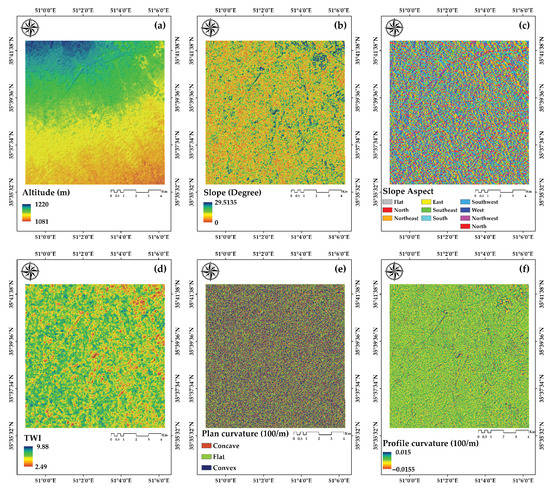
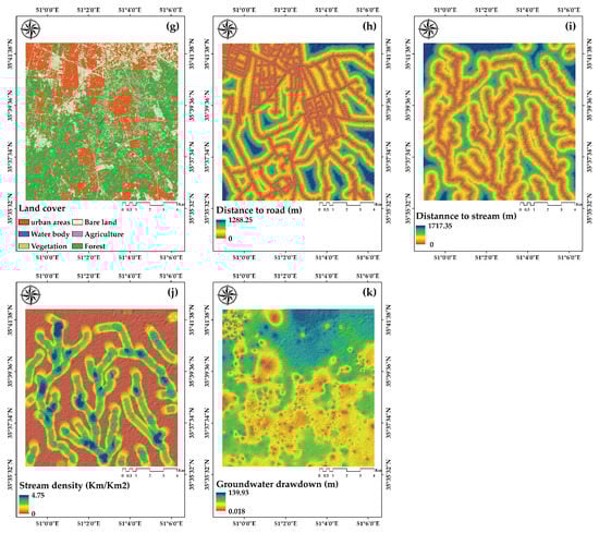
Figure 3.
Land subsidence conditioning factors: (a) altitude; (b) slope; (c) slope aspect; (d) topographic wetness index (TWI); (e) plan curvature; (f) profile curvature; (g) land cover; (h) distance to road; (i) distance to stream; (j) stream density and (k) groundwater drawdown.
3. Methodology
In this section, the methods and models used in different parts of the approach are presented in detail. First, the PS-InSAR technique used for generating land subsidence map of the study area and the LS inventory are discussed. Then, the ANFIS model and evolutionary algorithms, GWO and ICA, are stated. Moreover, FR analysis and the approach to optimize ANFIS using meta-heuristics are presented. Finally, the validation methodology of this paper is outlined.
3.1. PS-InSAR Technique
SAR Interferometry (InSAR) is a well-established technique for measuring and monitoring ground deformation with millimetric accuracy. This is mainly based on the phase difference between SAR images acquired at different times and slightly different sensor positions. Time-series InSAR analysis aims to identify coherent image pixels (persistent scatterers (PSs)), which have high phase stability and reflect strong backscatter to the satellite over a long time period. A baseline configuration can determine the set of interferometric image pairs, which is used in the time series analysis. The baseline shows the distance between two images, in terms of antenna position (spatial baseline), acquisition time (temporal baseline), or Doppler centroid (Doppler baseline). The single-master configuration, where each image is co-registered to a unique master image, is the most common one for PSI analysis [49,50]. The master image is chosen in the middle of the 2D spatio-temporal space so that the high coherence of all formed interferometric pairs (interferograms) is guaranteed. The interferogram contains the ground deformation phase component as well as some other distinct contributions, such as atmospheric disturbance, topographic, and flat-Earth terms. These components are removed in the next step from the interferometric phase using an external DEM.
A spatial network is formed using a primary set of points as PS candidates (PSCs) to estimate the Atmospheric Phase Screen (APS) and further densification of PS points. Since the original interferometric phase is wrapped (i.e., phase observations in the [)), and it is composed of a large number of phase contributions, the PSCs cannot be selected based on the phase. Thus, the amplitude dispersion index (ADI) based on Equation (1) is used as an approximation of phase stability. A point can be selected as a PSC if it always has a higher amplitude value than a suitable threshold. It was proved that assuming sufficient data images, the phase behavior with the standard deviation () lower than a threshold of 0.25 is similar to the trend of ADI. Hence, this index, which represents the phase stability of points, can be used for PSCs selection.
where is the standard deviation and is the average amplitude value of each pixel over time. Next, the spatial network is used to estimate the unknown parameters, DEM error (residual topographic phase component), and the deformation rate, along with each connection between two adjacent PSCs through the maximization of a periodogram (Equation (2)) [51]. All PSI methods are based on assumptions regarding the spatial and temporal smoothness of the deformation signal, expressed by a model. Here, the model is considered as a linear deformation trend in time.
where demonstrates the connection between adjacent PSCs and . N is the number of interferograms. The term is the double difference interferometric phase in image pairs s and k, while and are the temporal and interferometric normal baselines, respectively. refers to the incidence angle of the SAR signal.
For each PSC, the average residual phase after correction for the modeled parameters is taken to obtain an estimate for the atmospheric signal in the master image. Then, the atmospheric signal of the slave images as well as phase noise is separated from un-modeled deformation based on high-pass filtering. After APS removal, to increase point density, the second set of PSs is selected using a higher threshold for the ADI criterion. The unknown parameters are re-estimated for all pixels based on another maximization of the periodogram [49]. Eventually, temporal coherence, which is a function of residual phase noise, is used to determine the final PSs which build the land deformation map.
3.2. Adaptive Neuro-Fuzzy Inference System (ANFIS)
Fuzzy inference systems (FIS) are capable of depicting multifaceted processes using the concepts and if-then rules. However, they are incapable of learning [52]. Furthermore, if the number of input variables is too large, then selecting the membership functions and setting the fuzzy rules will become challenging [53]. On the other hand, learning algorithms automatically choose the suitable set of parameters for fuzzy membership functions despite their inability to explain the system under study. Thus, the ANFIS model [54] is a mixture of ANN and FL benefiting from both ANN’s computation capability and FL’s decision making. The structure of the ANFIS model contains five layers, called adaptive and fixed [55]. The ANFIS model employs the Takagi–Sugeno–Kang fuzzy algorithm in two rules of ‘if-then’ with two inputs, and , and one output for both as follows [56]:
Each node contains adaptive nodes, and input variables are fuzzified in first layer (Equations (5) and (6)):
where, x and y are the input nodes, A and B are the linguistic variables, and and are membership functions for that node. The second layer contains fixed nodes denoted as ᴫ to compute the strength of the rules. The output of each node is the product of all input signals to that node (Equation (7)):
where is the output for each node.
The third layer encompasses fixed nodes denoted as N. The nodes in this layer are the normalized outputs of the second layer, which are referred to as the normal firepower (Equation (8)):
All nodes in the fourth layer are adaptive and associated with a node function described by the following equation:
where is the normalized firepower of third layer and , , and are node parameters. The parameters of this layer are can be interpreted as the result parameters.
The final layer has only one node denoted as Ʃ, which represents the summation of all the input signals:
3.3. Imperialist Competitive Algorithm
The imperialist competitive algorithm (ICA) is a novel evolutionary algorithm based on human social evolution, developed by Atashpaz-Gargari and Lucas [57]. The ICA belongs to the group of swarm intelligence, which provides a powerful algorithm for solving NP-hard problems through its capability of dealing with continuous optimization. In this algorithm, the primary population is composed of several countries, and they interact with each other to form empires. Assuming the value of the objective function, colonialist and colonial groups are formed based on the existing countries. After ascertaining a colonialist, other countries are randomly allocated to one of the colonizers [57,58]. Every colonialist and its associated colony is called an empire. The algorithm then simulates the competition among imperialists in order to acquire more colonies. The best colonialist typically has more chance to occupy more colonies.
Another way of allocating the colonies to each colonialist is based on their normalized cost, which is calculated via Equation (11):
where is the empire’s total cost n, and is the total normalized cost value of that empire. Possession eventuality of the colonization competition by each empire is calculated by Equation (12):
The next phase is to attempt to approach a colonial country to analyze the colonies’ cultural and social structures in different political and social layers. The colonies then move to the colonialist country. The colonialist and colony will change their positions; the new colonialist position will continue with the algorithm. The new colonialist country will start applying adjustment to its colonies this time. To calculate the cost function, the total empire cost is given by Equation (13) as follows:
where f(imp) is the value of the cost function for the colonialist, f(colony) represents the mean values of the cost function for the colonies, and the constant ᵹ is considered a value between 0 and 1.
Finally, the cost of each empire is calculated, and the colonies of weak empires are abolished and join to stronger empires. This process of recruitment or competition between colonialists is continued. In the next stage, empires that have lost all their colonies will be eliminated and will join other colonies. The process is repeated until a single universal empire in the globe is built that is very close to the empire with colonial nations [59].
3.4. Grey Wolf Optimization
The novel grey wolf optimization (GWO) algorithm, presented by Mirjalili et al. [60], is an inspiration from the hunting behavior of grey wolves and the social hierarchy in nature. Wolves are social animals that live in packs, and they have a hierarchy consisting of four groups. The leader of each group, the alpha wolf (α), makes decisions about hunting, sleeping, and walking time, and all the other group members must follow its directives. In terms of hierarchy, the other wolves fall into three levels, called beta (β), delta (δ), and omega (ω). The beta wolves at the second level assist the alpha in making decisions and devise them. They are the best candidates for alpha replacement. Another notable characteristic is their group hunting, which can be summarized in four stages: (1) encircling prey, (2) hunting, (3) attacking prey (exploitation), and (4) searching for prey (exploring) [61]. The hunting process (optimization) is led by α, β, and δ wolves, and ω wolves have to abide by these three groups.
- 1.
- Encircling prey
In the first stage, the grey wolves encircle and surround the prey during hunting. To define this phase mathematically, the following Equations (14) and (15) are proposed. The parameter measures the distance between the grey wolf and the prey, and represents the location of the prey:
where denotes the current iteration, and and denote the position vectors of the prey and the grey wolves, respectively. The and coefficient vectors are defined as follows:
where components of are linearly decreased from 2 to 0 over the course of iterations, and r1 and r2 are random vectors between [0,1].
- 2.
- Hunting
After the encircling of the prey, the hunting phase is guided by α, β, and δ since they are supposed to have compressive knowledge about the prey’s position. This can be computed using following formulas:
where , , denote the position of α, β and δ, wolves respectively. , , and , , are the respective coefficient vectors. The position of a grey wolf in the search space can be updated as follows:
The other wolves update their positions randomly according to the position of the prey.
- 3.
- Attacking prey
The process of hunting ends when the prey stops moving and gray wolves attack the prey. It is important to note that the fluctuation range of is [−2a, 2a], where a is linearly decreased from 2 to 0. The exploration trend happens when < 1 and < 1. At this moment, the wolves attack the prey.
- 4.
- Search for prey
The grey wolves track and chase the prey. The pursuing of the prey is known as the exploration phase in the GWO algorithm [62]. The parameters α, β, and δ have guidance responsibility in this process. If > 1, it means the grey wolves are split and distributed in diverse ways for searching of the prey. After finding it, they congregate to attack. The coefficient provides a random weight for the prey while > 1 and promotes the exploration phase. In addition, models the natural hindrances in hunting for the grey wolves.
3.5. Frequency Ratio
One of the statistical bivariate models is FR, which is widely used in modeling environmental hazards as a geospatial assessment tool for quantifying the potential relationship between dependent and independent variables [63]. The FR value for a certain class from a given factor can be calculated using:
where is the number of pixels in each class of each factor with land subsidence locations. is the number of pixels of factor, m is the number of classes in the factor, and n is the number of factors in the study area [64].
3.6. ANFIS with Meta-Heuristic Algorithms
In ANFIS, parameter adjustment and the creation of a basic fuzzy system are done by combining traditional methods and then back error propagation. In this research, ICA and GWO were used as meta-heuristic algorithms to enhance the results of the ANFIS system and also to tweak the parameters of membership functions [52,65]. First, using input and target data, the FIS is created by the ANFIS model. Next, the membership functions are optimized and adjusted by meta-heuristic algorithms, and the output for the ANFIS (y) model is computed by [66]:
where is the target data, is a function of input data and optimized FIS, and is the error function that should be minimized. When the final conditions are met with the best output, the optimization process stops; otherwise, the membership function optimization is repeated.
3.7. Validation
In this research, the ROC curves were used for the accuracy assessment of the LSS models employed [6,10,39]. The ROC curve analysis is a common method to evaluate the goodness-of-fit and prediction power of models regarding the area under the curve (AUC) [2,67]. Ranging from 0 to 1, higher AUC values represent more reliable and accurate model performance. According to Yesilnacar [53], the qualitative relationship between AUC and the prediction accuracy of a model can be classified into the following categories: 0.5–0.6 (poor), 0.6–0.7 (average), 0.7–0.8 (good), 0.8–0.9 (very good), and 0.9–1 (excellent).
4. Results
By utilizing the spatial data and subsidence inventory generated and the methods discussed above, the mapping and assessment of land subsidence susceptibility for Shahryar County were conducted. In the following sub-sections, the results of the various parts of the methodology are thoroughly discussed.
4.1. Result of PS-InSAR
The ground deformation rate along the line of sight (LOS) direction during the acquisition time interval was obtained based on the PS-InSAR technique (see Section 3.1). SARPROZ (SAR PROcessing tool by periZ) [51] software was used to implement the PS-InSAR technique in the current research paper. The star configuration of the S-1A SLC time-series data stack is shown in Figure 4. The master image for the dataset was selected based on maximizing the stack coherence [68]. All slave images were co-registered with respect to the master image (2019/09/11). The shuttle radar topography mission (SRTM) DEM was used to remove topographic-related phase components from the interferometric phases. After the selection of 7881 PSCs, a spatial network was created by Delaunay Triangulation, connecting each point to the other. The unknown LOS velocity and DEM error were calculated along with the connections by maximizing a periodogram. All the obtained parameters were then integrated into the absolute values with respect to a reference point, which had no subsidence rate. The atmospheric phase for PSCs can be resampled on the uniform image grid as the APS. With having APS compensated for all slave images, the unknowns were estimated again for more PS points, selected by a lower threshold on ADI to obtain a more dense subsidence map. Figure 5a shows the LOS deformation map. According to Figure 5a, the maximum velocity was about −175 mm/year, which occurred in the southern agricultural part of the region of interest, where more ground-water extraction was observed.
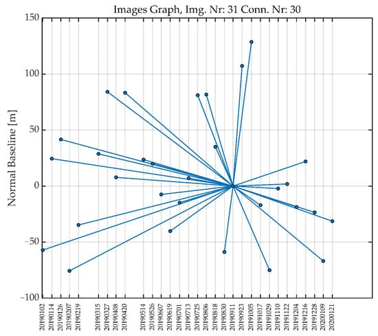
Figure 4.
The perpendicular baseline graph for the time-series data stack. The dots represents the images, and the edges denote the interferograms.
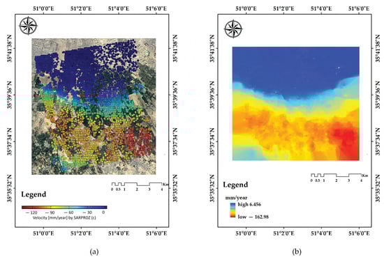
Figure 5.
(a) The annual velocity map based on the PSInSAR technique. The map is superimposed on the Google Earth (GE) imagery; (b) IDW interpolation raster of the velocity map.
Further, the LOS deformation rates should be decomposed into horizontal and vertical deformation components as it is the inherently vertical movement of the Earth’s surface with a slight horizontal displacement. It has been proved that the horizontal deformation is a very small portion of motion compared to the vertical deformation [67,69]. Hence, the LOS deformation could be assumed as negligible and converted simply into the vertical deformation rates using the cosine of the incidence angle of the radar signal. The interpolated land subsidence inventory map was designed based on the vertical velocity deformation map for Shahryar County, depicted in Figure 5b. ADI was more successful in identifying PS points in man-made areas with stable targets than agricultural areas [70]. Since vegetated regions are the main land cover in our case study, an interpolation was applied to the obtained vertical map to extend the deformation information for the whole study area. The inverse distance weighted (IDW) interpolation was used with a weighting power of 2 and neighboring radius of 12 for calculating the vertical velocity interpolation.
4.2. Result of FR
The results of the FR analysis in identifying the relationship of land subsidence occurrence with the conditioning factors are summarized in Table 3. Two out of five altitude classes had the highest probability (FR > 1.0), with 1119 to 1137 m being the most correlated class with land subsidence, followed by the altitude class lower than 1119 m. The results of the slope angle analysis showed that slopes ranging between 4.5 and 6.8 degrees had the highest FR (1.11). Further, a TWI class lower than 4.84, profile curvature higher than 0.0029, convex plan curvature class, and flat (F) slope aspect had the most influence on LSS for each corresponding factor. Land cover analysis results indicated that forest and urban classes had the highest probability of land subsidence occurrence, with FR values of 1.17 and 1.04, respectively. Distance to a stream of between 50 to 100 m had the highest FR, and the class of lower than 50 m had a considerable correlation; a stream density higher than 2.68 had the highest correlation with land subsidence and the 1.23 to 1.92 class, which also had a considerable FR value. For distance to road, the 0 to 100 m class had the highest FR followed by the 100 to 200 m classes. Finally, groundwater drawdown ranging from 55 to 83 m and from 28 to 55 m had higher impacts on land subsidence occurrence.
Table 3.
Relationship between land subsidence occurrence and conditioning factors using the FR model.
4.3. Result of Hybrid Models
In the course of implementation of the hybrid models, 70% of the land subsidence points (210 locations) were used for training with values 1, and the same number of randomly selected non-subsidence points were taken into account with 0 values in the training phase. For the test dataset, 30% of the subsidence inventory (90 locations) with a value of 1 was used, with 90 randomly assigned points with a value of 0. The training datasets were used to calibrate the weights of the membership functions. The testing dataset was used to evaluate the performance of the trained ANFIS ensemble models. Hybrid models were implemented in MATLAB 2017b software. The parameters used in meta-heuristic algorithms are presented in Table 4. The prediction power of ANFIS and the two hybrid models with the training dataset (target) along with the comparison of the output and target testing dataset is shown in Figure 6.
Table 4.
Parameters used in hybrid algorithms.
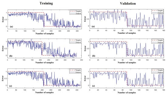
Figure 6.
The target and output values for training and validation datasets of (a) ANFIS, (b) ANFIS-GWO, and (c) ANFIS-ICA.
The RMSEs of the training and testing phases were calculated and are shown in Table 5. The two ensemble models enhanced the ANFIS model, and the ANFIS-ICA outperformed the ANFIS-GWO with an RMSE of 0.276 in the training phase and 0.3199 in the validation and testing phase. The ANFIS-GWO yielded an RMSE of 0.313 and 0.3217 in training and validation phases, respectively. Finally, the ANFIS model resulted in 0.323 in training and 0.34 in the validation phase.
Table 5.
The comparison of model performance.
The convergence results of the two ANFIS-ICA and ANFIS-GWO ensemble models up to 1000 iterations are shown in Figure 7. ANFIS-ICA had a better convergence value (0.276) than ANFIS-GWO (0.313). The lowest amount of the cost function (RMSE) indicates the best cost and thus the best performance in predicting the results.
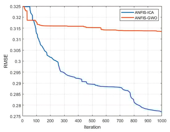
Figure 7.
The convergence graph of the objective functions.
4.4. LSSM Using ANFIS and Its Optimized Models
The original ANFIS and its optimized ensembles in this research were trained and used to estimate land subsidence susceptibility in the study area. Susceptibility modelling and estimation were all carried out in MATLAB 2017b and were then exported to ArcGIS 10.3 software to classify and generate the susceptibility maps. Land susceptibility index was classified into five classes, very high, high, moderate, low, and very low, based on a natural break classification scheme [22,41]. Figure 8 presents the generated classified subsidence susceptibility maps obtained from ANFIS, ANFIS-GWO, and ANFIS-ICA. As can be seen, all the output subsidence susceptibility maps are similar and consistent with each other, particularly the ones for ANFIS-ICA and ANFIS-GWO. Moreover, the map based on ANFIS-ICA is much smoother than the others.
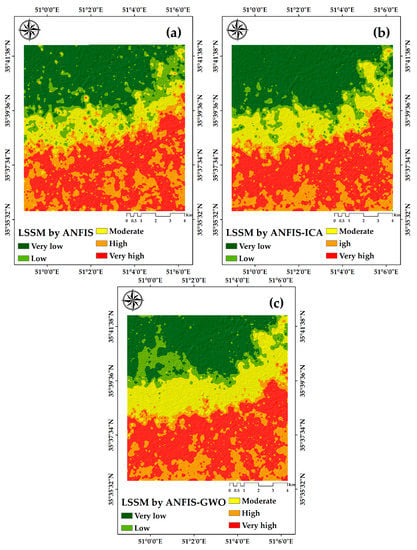
Figure 8.
The LSS maps of the study area using (a) ANFIS, (b) ANFIS-ICA, and (c) ANFIS-GWO.
4.5. Validation
The ROC curves were calculated for all LSS maps using the test data. Figure 9 demonstrates the comparison of AUC for all the models used. The results showed that the ANFIS-ICA had the highest prediction accuracy (0.932), followed by the ANFIS-GWO (0.926) and ANFIS (0.908). This proves that the combination of the ANFIS model with meta-heuristic algorithms such as GWO and ICA can significantly improve the output land subsidence susceptibility maps in comparison to ANFIS alone.
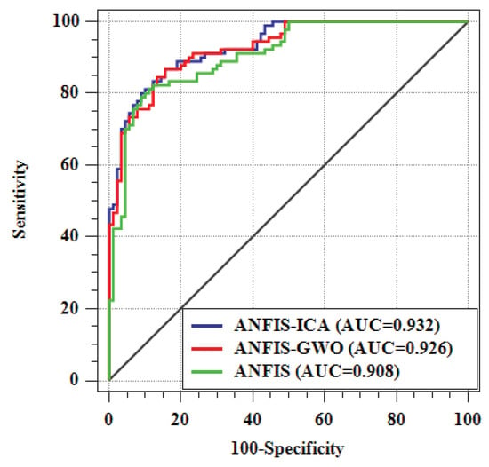
Figure 9.
The ROC curves for the LSSMs of the models and their AUC.
5. Discussion
Land subsidence is the slow vertical lowering of the Earth’s surface, posing a serious threat to both the environment and human life. Recently, there has been an increasing interest in land subsidence analysis and monitoring in Iran as it is one of the highest subsidence-prone countries [17,18,20,24]. Natural hazard vulnerability analysis using machine learning algorithms (i.e., ANFIS) has shown promising results. Therefore, in this research, the focus was to employ the ANFIS model in combination with meta-heuristics in land subsidence susceptibility mapping.
Land subsidence inventories are necessary for accurate subsidence susceptibility analysis. The use of remote sensing SAR data is suitable for providing subsidence inventories due to their wide availability, independence from fieldwork, time and cost efficiency, frequent repeatability over time, and, especially, high precision [6]. In this work, the PS-InSAR technique with its millimetric precision was employed to determine the subsided areas in the region of interest to form the inventory data used for training and testing the LSS models.
Important conditioning factors for determining land subsidence prone areas were identified and collected based on either the literature or availability of data. The FR model was used to evaluate the correlation and influence of the factors. The results showed that all the factors employed in this paper had a considerable effect on LSS in Shahryar County. Among all the factors, the flat (slope aspect) area had the highest FR value (3.7), indicating high subsidence susceptibility in flat areas. The slope angle is related to the hydro physiographic characteristics that can influence the water infiltration rate and the volume and velocity of the Earth’s surface flow [13]. Altitude and groundwater drawdown were the best predictors of land subsidence in this study, followed by stream density and distance to stream. Rahmati et al. and Arabameri et al. [2,37] also found that groundwater drawdown had a greater impact on land subsidence. Other topo-hydrographic factors, such as stream density and distance to stream are indirectly related to LS as they impact groundwater recharge and infiltration [2,40] and, as can be seen in the results, the land areas closer to streams and with a certain stream density were more susceptible to LS. In terms of altitude, the lower lands were more prone to subsidence as the class 1137 to 1119 m and those lower than 1119 m had the highest FR. TWI, plan curvature, and profile curvature are among secondary topographic derivatives indirectly influencing LS [2,40,71]. These factors were not among best predictors of subsidence in the study area, which may be due to smooth and low altitude changes in the study area. The FR analysis showed that a TWI lower than 4.84 was strongly correlated with LS. In a similar study [40], lower TWI values (i.e., 2.54 to 8) have been reported to be more prone to subsidence. Positive and convex plan and profile curvatures had the highest FR value, as reported in [40]. Cropland and urban land cover types exist in lower altitude and flat areas. The main water source of the area is groundwater; therefore, more extraction of water in recent years as a result of population increase has caused the subsidence rate to increase. Previous studies have stressed the impact of groundwater extraction on subsidence occurrence [72,73]. Regarding the distance to road factor, the closer to a road, the greater the land subsidence risk, which can be due to closeness to urban land cover and thus indirectly related to the subsidence phenomenon.
Two novel meta-heuristic algorithms, GWO and ICA, were used to optimize the rules and parameters of the ANFIS model. Both of these evolutionary algorithms belong to swarm intelligence. The results showed that ICA had a slower convergence rate than GWO; however, it had better performance. In order to evaluate the prediction power and accuracy of the models, RMSE and ROC criteria were used. The RMSE is simply based on error assessment, whereas ROC is based on true positive (TP), false positive (FP), true negative (TN), and false negative (FN), which is more appropriate for comparison [42]. ANFIS-ICA had the lowest RMSE in both the training (0.276) and testing (0.3199) phases, followed by ANFIS-GWO and ANFIS alone. According to the AUC-ROC results, the ANFIS-ICA model was more accurate (0.932), followed by the ANFIS-GWO model (0.926) and the ANFIS model (0.908). It can be seen that the use of machine learning algorithms resulted in higher prediction accuracy since ANFIS alone yielded a suitable performance compared to other statistical methods in other studies. It can also be concluded that optimization of the ANFIS algorithm by meta-heuristics improves its results considerably. This was also reported in cases of other applications [64,74]. The results showed that the ICA algorithm was more accurate than the GWO algorithm in optimization of the ANFIS model. The advantages of the ICA algorithm are high convergence speed and the ability to optimize functions with a large number of variables [75]. The GWO algorithm has a small number of disadvantages, including a low solving accuracy, poor local searching ability, and slow convergence rate [60].
The output land subsidence susceptibility maps of the three models were similar and in line with each other. However, the map produced by the ANFIS-ICA was smoother than that of the other two. As could be observed, the high-risk areas were predicted where the groundwater extraction was higher, elevation was lower, and agricultural land use was higher. This is because the main source of income in the study area is agriculture. Further, the population has increased; therefore, food production has stressed the groundwater, the main water source of the area, and thus the land subsidence risk has become higher in those areas. Further, it is evident that the subsidence trend is gradually reaching towards the urban part of the Shahryar County, posing a serious threat to settlements and human life. The generated LSSMs in this paper can benefit authorities and decision-makers to identify subsidence-prone areas regarding environmental and urban management.
6. Conclusions
Land subsidence is an important issue in Iran due to the semi-arid and arid climate and excessive groundwater extraction. Therefore, modeling, simulation, and risk mapping offer valuable knowledge of environmental geohazards. GIS-based predictions have proved to be essential for authorities in terms of planning and decision-making. In this work, we used remote sensing SAR data and the PSInSAR technique to create a land subsidence inventory of the study area as a high-precision tool with a low cost and frequent reproducibility. Since machine learning tools have shown appropriate performance in modeling and mapping hazard susceptibility, the ANFIS model was used in this research to map the land subsidence risk in Shahryar County, Tehran province, Iran. Another objective of this paper was to investigate the effect of optimization of the ANFIS model through meta-heuristics. Two novel evolutionary algorithms, namely, GWO and ICA, were used to create ensemble models. The results of the three models in both training and testing phases were assessed by RMSE. In both phases, ANFIS-ICA had the lowest RMSE, followed by ANFIS-GWO and ANFIS alone. AUC-ROC analysis was also used for model evaluation, and its results indicated that ANFIS-ICA had the best prediction performance (0.932), followed by ANFIS-GWO (0.926) and ANFIS (0.908). To conclude, the results overall showed the applicability of the ANFIS machine learning algorithm in land subsidence susceptibility mapping and the effectiveness of its ensembles with meta-heuristic algorithms. The methodology used is reproducible and can be applied to other regions with different environmental parameters to test the modelling performance. Further studies should be applied using other machine learning and deep learning algorithms to compare their prediction accuracy. In addition, future research can focus on developing risk monitoring and early-warning frameworks.
Author Contributions
Conceptualization, B.R. and S.V.R.-T.; Data curation, B.R. and S.V.R.-T.; methodology, S.V.R.-T., F.F. and B.R.; software, D.P., F.F. and S.V.R.-T.; validation, S.V.R.-T., F.F. and B.R.; formal analysis, B.R., S.V.R.-T., F.F., A.S.-N. and D.P.; investigation, B.R.; resources, F.F.; writing—original draft preparation, B.R.; writing—review and editing, B.R., S.V.R.-T. and F.F.; visualization, S.V.R.-T. and B.R.; supervision, A.S.-N. and D.P.; project administration, F.F., A.S.-N. and D.P. All authors have read and agreed to the published version of the manuscript.
Funding
This research received no external funding.
Acknowledgments
The authors would like to thank the European Space Agency (ESA) for freely providing Sentinel-1 satellite imagery.
Conflicts of Interest
The authors declare no conflict of interest.
References
- Holzer, T.L.; Galloway, D.L. Impacts of land subsidence caused by withdrawal of underground fluids in the United States. Hum. Geol. Agents 2005, 16, 87–99. [Google Scholar]
- Arabameri, A.; Saha, S.; Roy, J.; Tiefenbacher, J.P.; Cerda, A.; Biggs, T.; Pradhan, B.; Thi Ngo, P.T.; Collins, A.L. A novel ensemble computational intelligence approach for the spatial prediction of land subsidence susceptibility. Sci. Total Environ. 2020, 726, 138595. [Google Scholar] [CrossRef] [PubMed]
- Raspini, F.; Bianchini, S.; Moretti, S.; Loupasakis, C.; Rozos, D.; Duro, J.; Garcia, M. Advanced interpretation of interferometric SAR data to detect, monitor and model ground subsidence: Outcomes from the ESA-GMES Terrafirma project. Nat. Hazards 2016, 83, 155–181. [Google Scholar] [CrossRef]
- Galloway, D.L.; Burbey, T.J. Review: Regional land subsidence accompanying groundwater extraction. Hydrogeol. J. 2011, 19, 1459–1486. [Google Scholar] [CrossRef]
- Xue, Y.-Q.; Zhang, Y.; Ye, S.-J.; Wu, J.-C.; Li, Q.-F. Land subsidence in China. Environ. Geol. 2005, 48, 713–720. [Google Scholar] [CrossRef]
- Bianchini, S.; Solari, L.; Del Soldato, M.; Raspini, F.; Montalti, R.; Ciampalini, A.; Casagli, N. Ground Subsidence Susceptibility (GSS) Mapping in Grosseto Plain (Tuscany, Italy) Based on Satellite InSAR Data Using Frequency Ratio and Fuzzy Logic. Remote Sens. 2019, 11, 2015. [Google Scholar] [CrossRef]
- Shi, X.; Jiang, S.; Xu, H.; Jiang, F.; He, Z.; Wu, J. The effects of artificial recharge of groundwater on controlling land subsidence and its influence on groundwater quality and aquifer energy storage in Shanghai, China. Environ. Earth Sci. 2016, 75, 195. [Google Scholar] [CrossRef]
- Modoni, G.; Darini, G.; Spacagna, R.L.; Saroli, M.; Russo, G.; Croce, P. Spatial analysis of land subsidence induced by groundwater withdrawal. Eng. Geol. 2013, 167, 59–71. [Google Scholar] [CrossRef]
- Stanley, J.-D.; Corwin, K.A. Measuring Strata Thicknesses in Cores to Assess Recent Sediment Compaction and Subsidence of Egypt’s Nile Delta Coastal Margin. J. Coast. Res. 2012, 29, 657–670. [Google Scholar] [CrossRef]
- Tien Bui, D.; Shahabi, H.; Shirzadi, A.; Chapi, K.; Pradhan, B.; Chen, W.; Khosravi, K.; Panahi, M.; Bin Ahmad, B.; Saro, L. Land Subsidence Susceptibility Mapping in South Korea Using Machine Learning Algorithms. Sensors 2018, 18, 2464. [Google Scholar] [CrossRef]
- Pradhan, B.; Abokharima, M.H.; Jebur, M.N.; Tehrany, M.S. Land subsidence susceptibility mapping at Kinta Valley (Malaysia) using the evidential belief function model in GIS. Nat. Hazards 2014, 73, 1019–1042. [Google Scholar] [CrossRef]
- Lee, S.; Park, I. Application of decision tree model for the ground subsidence hazard mapping near abandoned underground coal mines. J. Environ. Manag. 2013, 127, 166–176. [Google Scholar] [CrossRef] [PubMed]
- Mohammady, M.; Pourghasemi, H.R.; Amiri, M. Land subsidence susceptibility assessment using random forest machine learning algorithm. Environ. Earth Sci. 2019, 78, 503. [Google Scholar] [CrossRef]
- Fiaschi, S.; Tessitore, S.; Bonì, R.; Di Martire, D.; Achilli, V.; Borgstrom, S.; Ibrahim, A.; Floris, M.; Meisina, C.; Ramondini, M.; et al. From ERS-1/2 to Sentinel-1: Two decades of subsidence monitored through A-DInSAR techniques in the Ravenna area (Italy). GIScience Remote Sens. 2017, 54, 305–328. [Google Scholar] [CrossRef]
- Galloway, D.L.; Jones, D.R.; Ingebritsen, S.E. Land Subsidence in the United States; US Geological Survey: Reston, VA, USA, 1999; Volume 1182.
- Conway, B.D. Land subsidence and earth fissures in south-central and southern Arizona, USA. Hydrogeol. J. 2016, 24, 649–655. [Google Scholar] [CrossRef]
- Mahmoudpour, M.; Khamehchiyan, M.; Nikudel, M.R.; Ghassemi, M.R. Numerical simulation and prediction of regional land subsidence caused by groundwater exploitation in the southwest plain of Tehran, Iran. Eng. Geol. 2016, 201, 6–28. [Google Scholar] [CrossRef]
- Motagh, M.; Walter, T.R.; Sharifi, M.A.; Fielding, E.; Schenk, A.; Anderssohn, J.; Zschau, J. Land subsidence in Iran caused by widespread water reservoir overexploitation. Geophys. Res. Lett. 2008, 35, L16403. [Google Scholar] [CrossRef]
- Dehghani, M.; Valadan Zoej, M.J.; Hooper, A.; Hanssen, R.F.; Entezam, I.; Saatchi, S. Hybrid conventional and Persistent Scatterer SAR interferometry for land subsidence monitoring in the Tehran Basin, Iran. ISPRS J. Photogramm. Remote Sens. 2013, 79, 157–170. [Google Scholar] [CrossRef]
- Tarighat, F.; Foroughnia, F.; Perissin, D. Monitoring of Power Towers’ Movement Using Persistent Scatterer SAR Interferometry in South West of Tehran. Remote Sens. 2021, 13, 407. [Google Scholar] [CrossRef]
- Rahmati, O.; Golkarian, A.; Biggs, T.; Keesstra, S.; Mohammadi, F.; Daliakopoulos, I.N. Land subsidence hazard modeling: Machine learning to identify predictors and the role of human activities. J. Environ. Manag. 2019, 236, 466–480. [Google Scholar] [CrossRef] [PubMed]
- Ghorbanzadeh, O.; Feizizadeh, B.; Blaschke, T. An interval matrix method used to optimize the decision matrix in AHP technique for land subsidence susceptibility mapping. Environ. Earth Sci. 2018, 77, 584. [Google Scholar] [CrossRef]
- Ebrahimy, H.; Feizizadeh, B.; Salmani, S.; Azadi, H. A comparative study of land subsidence susceptibility mapping of Tasuj plane, Iran, using boosted regression tree, random forest and classification and regression tree methods. Environ. Earth Sci. 2020, 79, 223. [Google Scholar] [CrossRef]
- Foroughnia, F.; Nemati, S.; Maghsoudi, Y.; Perissin, D. An iterative PS-InSAR method for the analysis of large spatio-temporal baseline data stacks for land subsidence estimation. Int. J. Appl. Earth Obs. Geoinf. 2019, 74, 248–258. [Google Scholar] [CrossRef]
- Chaussard, E.; Wdowinski, S.; Cabral-Cano, E.; Amelung, F. Land subsidence in central Mexico detected by ALOS InSAR time-series. Remote Sens. Environ. 2014, 140, 94–106. [Google Scholar] [CrossRef]
- Wang, Q.; Li, W. A GIS-based comparative evaluation of analytical hierarchy process and frequency ratio models for landslide susceptibility mapping. Phys. Geogr. 2017, 38, 318–337. [Google Scholar] [CrossRef]
- Choi, J.-K.; Kim, K.-D.; Lee, S.; Won, J.-S. Application of a fuzzy operator to susceptibility estimations of coal mine subsidence in Taebaek City, Korea. Environ. Earth Sci. 2010, 59, 1009–1022. [Google Scholar] [CrossRef]
- Zhou, G.; Yan, H.; Chen, K.; Zhang, R. Spatial analysis for susceptibility of second-time karst sinkholes: A case study of Jili Village in Guangxi, China. Comput. Geosci. 2016, 89, 144–160. [Google Scholar] [CrossRef]
- Lee, S.; Park, I.; Choi, J.-K. Spatial prediction of ground subsidence susceptibility using an artificial neural network. Environ. Manag. 2012, 49, 347–358. [Google Scholar] [CrossRef]
- Rafie, M.; Samimi Namin, F. Prediction of subsidence risk by FMEA using artificial neural network and fuzzy inference system. Int. J. Min. Sci. Technol. 2015, 25, 655–663. [Google Scholar] [CrossRef]
- Hu, B.; Zhou, J.; Wang, J.; Chen, Z.; Wang, D.; Xu, S. Risk assessment of land subsidence at Tianjin coastal area in China. Environ. Earth Sci. 2009, 59, 269. [Google Scholar] [CrossRef]
- Rezaei, M.; Yazdani Noori, Z.; Dashti Barmaki, M. Land subsidence susceptibility mapping using Analytical Hierarchy Process (AHP) and Certain Factor (CF) models at Neyshabur plain, Iran. Geocarto Int. 2020, 1–17. [Google Scholar] [CrossRef]
- Ghorbanzadeh, O.; Blaschke, T.; Aryal, J.; Gholaminia, K. A new GIS-based technique using an adaptive neuro-fuzzy inference system for land subsidence susceptibility mapping. J. Spat. Sci. 2020, 65, 401–418. [Google Scholar] [CrossRef]
- Abdollahi, S.; Pourghasemi, H.R.; Ghanbarian, G.A.; Safaeian, R. Prioritization of effective factors in the occurrence of land subsidence and its susceptibility mapping using an SVM model and their different kernel functions. Bull. Eng. Geol. Environ. 2019, 78, 4017–4034. [Google Scholar] [CrossRef]
- Taravatrooy, N.; Nikoo, M.R.; Sadegh, M.; Parvinnia, M. A hybrid clustering-fusion methodology for land subsidence estimation. Nat. Hazards 2018, 94, 905–926. [Google Scholar] [CrossRef]
- Pourghasemi, H.R.; Mohseni Saravi, M. Land-Subsidence Spatial Modeling Using the Random Forest Data-Mining Technique. In Spatial Modeling in GIS and R for Earth and Environmental Sciences; Elsevier: Amsterdam, The Netherlands, 2019; pp. 147–159. [Google Scholar]
- Rahmati, O.; Falah, F.; Naghibi, S.A.; Biggs, T.; Soltani, M.; Deo, R.C.; Cerdà, A.; Mohammadi, F.; Tien Bui, D. Land subsidence modelling using tree-based machine learning algorithms. Sci. Total Environ. 2019, 672, 239–252. [Google Scholar] [CrossRef]
- Tomás, R.; Romero, R.; Mulas, J.; Marturià, J.J.; Mallorquí, J.J.; Lopez-Sanchez, J.M.; Herrera, G.; Gutiérrez, F.; González, P.J.; Fernández, J.; et al. Radar interferometry techniques for the study of ground subsidence phenomena: A review of practical issues through cases in Spain. Environ. Earth Sci. 2014, 71, 163–181. [Google Scholar] [CrossRef]
- Del Soldato, M.; Farolfi, G.; Rosi, A.; Raspini, F.; Casagli, N. Subsidence Evolution of the Firenze–Prato–Pistoia Plain (Central Italy) Combining PSI and GNSS Data. Remote Sens. 2018, 10, 1146. [Google Scholar] [CrossRef]
- Hakim, W.; Achmad, A.; Lee, C.-W. Land Subsidence Susceptibility Mapping in Jakarta Using Functional and Meta-Ensemble Machine Learning Algorithm Based on Time-Series InSAR Data. Remote Sens. 2020, 12, 3627. [Google Scholar] [CrossRef]
- Polykretis, C.; Chalkias, C.; Ferentinou, M. Adaptive neuro-fuzzy inference system (ANFIS) modeling for landslide susceptibility assessment in a Mediterranean hilly area. Bull. Eng. Geol. Environ. 2019, 78, 1173–1187. [Google Scholar] [CrossRef]
- Termeh, S.V.R.; Khosravi, K.; Sartaj, M.; Keesstra, S.D.; Tsai, F.T.-C.; Dijksma, R.; Pham, B.T. Optimization of an adaptive neuro-fuzzy inference system for groundwater potential mapping. Hydrogeol. J. 2019, 27, 2511–2534. [Google Scholar] [CrossRef]
- Oh, H.-J.; Ahn, S.-C.; Choi, J.-K.; Lee, S. Sensitivity analysis for the GIS-based mapping of the ground subsidence hazard near abandoned underground coal mines. Environ. Earth Sci. 2011, 64, 347–358. [Google Scholar] [CrossRef]
- Pacheco-Martínez, J.; Cabral-Cano, E.; Wdowinski, S.; Hernández-Marín, M.; Ortiz-Lozano, J.; Zermeño-de-León, M. Application of InSAR and Gravimetry for Land Subsidence Hazard Zoning in Aguascalientes, Mexico. Remote Sens. 2015, 7, 17035–17050. [Google Scholar] [CrossRef]
- Arabameri, A.; Lee, S.; Tiefenbacher, J.P.; Ngo, P.T.T. Novel Ensemble of MCDM-Artificial Intelligence Techniques for Groundwater-Potential Mapping in Arid and Semi-Arid Regions (Iran). Remote Sens. 2020, 12, 490. [Google Scholar] [CrossRef]
- Amani, M.; Ghorbanian, A.; Ahmadi, S.A.; Kakooei, M.; Moghimi, A.; Mirmazloumi, S.M.; Alizadeh Moghaddam, S.H.; Mahdavi, S.; Ghahremanloo, M.; Parsian, S.; et al. Google Earth Engine Cloud Computing Platform for Remote Sensing Big Data Applications: A Comprehensive Review. IEEE J. Sel. Top. Appl. Earth Obs. Remote Sens. 2020, 13, 5326–5350. [Google Scholar] [CrossRef]
- Amani, M.; Kakooei, M.; Moghimi, A.; Ghorbanian, A.; Ranjgar, B.; Mahdavi, S.; Davidson, A.; Fisette, T.; Rollin, P.; Brisco, B.; et al. Application of Google Earth Engine Cloud Computing Platform, Sentinel Imagery, and Neural Networks for Crop Mapping in Canada. Remote Sens. 2020, 12, 3561. [Google Scholar] [CrossRef]
- Ghorbanian, A.; Kakooei, M.; Amani, M.; Mahdavi, S.; Mohammadzadeh, A.; Hasanlou, M. Improved land cover map of Iran using Sentinel imagery within Google Earth Engine and a novel automatic workflow for land cover classification using migrated training samples. ISPRS J. Photogramm. Remote Sens. 2020, 167, 276–288. [Google Scholar] [CrossRef]
- Ferretti, A.; Prati, C.; Rocca, F. Permanent scatterers in SAR interferometry. IEEE Trans. Geosci. Remote Sens. 2001, 39, 8–20. [Google Scholar] [CrossRef]
- Kampes, B.M. Radar Interferometry; Springer: Dordrecht, The Netherlands, 2006. [Google Scholar]
- Perissin, D.; Wang, Z.; Lin, H. Shanghai subway tunnels and highways monitoring through Cosmo-SkyMed Persistent Scatterers. ISPRS J. Photogramm. Remote Sens. 2012, 73, 58–67. [Google Scholar] [CrossRef]
- Razavi Termeh, S.V.; Kornejady, A.; Pourghasemi, H.R.; Keesstra, S. Flood susceptibility mapping using novel ensembles of adaptive neuro fuzzy inference system and metaheuristic algorithms. Sci. Total Environ. 2018, 615, 438–451. [Google Scholar] [CrossRef]
- Yesilnacar, E.; Topal, T. Landslide susceptibility mapping: A comparison of logistic regression and neural networks methods in a medium scale study, Hendek region (Turkey). Eng. Geol. 2005, 79, 251–266. [Google Scholar] [CrossRef]
- Jang, J.-S.R. ANFIS: Adaptive-network-based fuzzy inference system. IEEE Trans. Syst. Man. Cybern. 1993, 23, 665–685. [Google Scholar] [CrossRef]
- Tien Bui, D.; Pradhan, B.; Lofman, O.; Revhaug, I.; Dick, O.B. Landslide susceptibility mapping at Hoa Binh province (Vietnam) using an adaptive neuro-fuzzy inference system and GIS. Comput. Geosci. 2012, 45, 199–211. [Google Scholar] [CrossRef]
- Takagi, T.; Sugeno, M. Fuzzy identification of systems and its applications to modeling and control. IEEE Trans. Syst. Man. Cybern. 1985, SMC-15, 116–132. [Google Scholar] [CrossRef]
- Atashpaz-Gargari, E.; Lucas, C. Imperialist competitive algorithm: An algorithm for optimization inspired by imperialistic competition. In Proceedings of the 2007 IEEE Congress on Evolutionary Computation, Singapore, 25–28 September 2007; pp. 4661–4667. [Google Scholar]
- Razavi-Termeh, S.V.; Sadeghi-Niaraki, A.; Choi, S.-M. Gully erosion susceptibility mapping using artificial intelligence and statistical models. Geomat. Nat. Hazards Risk 2020, 11, 821–844. [Google Scholar] [CrossRef]
- Esmaeil, A.G.; Farzad, H.; Ramin, R.; Caro, L. Colonial competitive algorithm: A novel approach for PID controller design in MIMO distillation column process. Int. J. Intell. Comput. Cybern. 2008, 1, 337–355. [Google Scholar] [CrossRef]
- Mirjalili, S.; Mirjalili, S.M.; Lewis, A. Grey Wolf Optimizer. Adv. Eng. Softw. 2014, 69, 46–61. [Google Scholar] [CrossRef]
- Rahmati, O.; Darabi, H.; Panahi, M.; Kalantari, Z.; Naghibi, S.A.; Ferreira, C.S.S.; Kornejady, A.; Karimidastenaei, Z.; Mohammadi, F.; Stefanidis, S.; et al. Development of novel hybridized models for urban flood susceptibility mapping. Sci. Rep. 2020, 10, 12937. [Google Scholar] [CrossRef]
- Chen, W.; Hong, H.; Panahi, M.; Shahabi, H.; Wang, Y.; Shirzadi, A.; Pirasteh, S.; Alesheikh, A.A.; Khosravi, K.; Panahi, S.; et al. Spatial Prediction of Landslide Susceptibility Using GIS-Based Data Mining Techniques of ANFIS with Whale Optimization Algorithm (WOA) and Grey Wolf Optimizer (GWO). Appl. Sci. 2019, 9, 3755. [Google Scholar] [CrossRef]
- Rahmati, O.; Pourghasemi, H.R.; Zeinivand, H. Flood susceptibility mapping using frequency ratio and weights-of-evidence models in the Golastan Province, Iran. Geocarto Int. 2016, 31, 42–70. [Google Scholar] [CrossRef]
- Regmi, A.D.; Devkota, K.C.; Yoshida, K.; Pradhan, B.; Pourghasemi, H.R.; Kumamoto, T.; Akgun, A. Application of frequency ratio, statistical index, and weights-of-evidence models and their comparison in landslide susceptibility mapping in Central Nepal Himalaya. Arab. J. Geosci. 2014, 7, 725–742. [Google Scholar] [CrossRef]
- Razavi-Termeh, S.V.; Khosravi, K.; Sadeghi-Niaraki, A.; Choi, S.-M.; Singh, V.P. Improving groundwater potential mapping using metaheuristic approaches. Hydrol. Sci. J. 2020, 65, 2729–2749. [Google Scholar] [CrossRef]
- Razavi-Termeh, S.V.; Sadeghi-Niaraki, A.; Choi, S.-M. Ubiquitous GIS-Based Forest Fire Susceptibility Mapping Using Artificial Intelligence Methods. Remote Sens. 2020, 12, 1689. [Google Scholar] [CrossRef]
- Pepe, A.; Bonano, M.; Zhao, Q.; Yang, T.; Wang, H. The Use of C-/X-Band Time-Gapped SAR Data and Geotechnical Models for the Study of Shanghai’s Ocean-Reclaimed Lands through the SBAS-DInSAR Technique. Remote Sens. 2016, 8, 911. [Google Scholar] [CrossRef]
- Kampes, B.M. Displacement Parameter Estimation Using Permanent Scatterer Interferometry. Ph.D. Thesis, Delft University of Technology, Delft, The Netherlands, September 2005. [Google Scholar]
- Ren, H.; Feng, X. Calculating vertical deformation using a single InSAR pair based on singular value decomposition in mining areas. Int. J. Appl. Earth Obs. Geoinf. 2020, 92, 102115. [Google Scholar] [CrossRef]
- Hooper, A.; Segall, P.; Zebker, H. Persistent scatterer interferometric synthetic aperture radar for crustal deformation analysis, with application to Volcán Alcedo, Galápagos. J. Geophys. Res. Solid Earth 2007, 112, B07407. [Google Scholar] [CrossRef]
- Pourghasemi, H.R.; Beheshtirad, M. Assessment of a data-driven evidential belief function model and GIS for groundwater potential mapping in the Koohrang Watershed, Iran. Geocarto Int. 2015, 30, 662–685. [Google Scholar] [CrossRef]
- Ye, S.; Xue, Y.; Wu, J.; Yan, X.; Yu, J. Progression and mitigation of land subsidence in China. Hydrogeol. J. 2016, 24, 685–693. [Google Scholar] [CrossRef]
- Suganthi, S.; Elango, L.; Subramanian, S.K. Microwave D-InSAR technique for assessment of land subsidence in Kolkata city, India. Arab. J. Geosci. 2017, 10, 458. [Google Scholar] [CrossRef]
- Moayedi, H.; Mehrabi, M.; Bui, D.T.; Pradhan, B.; Foong, L.K. Fuzzy-metaheuristic ensembles for spatial assessment of forest fire susceptibility. J. Environ. Manag. 2020, 260, 109867. [Google Scholar] [CrossRef]
- Pourghasemi, H.R.; Razavi-Termeh, S.V.; Kariminejad, N.; Hong, H.; Chen, W. An assessment of metaheuristic approaches for flood assessment. J. Hydrol. 2020, 582, 124536. [Google Scholar] [CrossRef]
Publisher’s Note: MDPI stays neutral with regard to jurisdictional claims in published maps and institutional affiliations. |
© 2021 by the authors. Licensee MDPI, Basel, Switzerland. This article is an open access article distributed under the terms and conditions of the Creative Commons Attribution (CC BY) license (https://creativecommons.org/licenses/by/4.0/).