Article

Predicting Skipjack Tuna Fishing Grounds in the Western and Central Pacific Ocean Based on High-Spatial-Temporal-Resolution Satellite Data

1
Institute of Ocean Technology and Marine Affairs, National Cheng Kung University, No. 1, University Road, Tainan City 70101, Taiwan
2
Graduate Institute of Marine Affairs, National Sun Yat-sen University, No. 70, Lienhai Rd., Kaohsiung City 80424, Taiwan
3
College of Ocean Science and Resources, National Taiwan Ocean University, No. 2, Pei-Ning Rd, Keelung City 20224, Taiwan
4
Information Division Overseas Fisheries Development Council, No. 19, Lane 113 Roosevelt Rd., Sec. 4, Taipei City 10673, Taiwan
5
Department of Hydraulic and Ocean Engineering, National Cheng Kung University, No. 1, University Road, Tainan City 70101, Taiwan
*
Author to whom correspondence should be addressed.
Remote Sens. 2021, 13(5), 861; https://doi.org/10.3390/rs13050861
Submission received: 17 January 2021 / Revised: 22 February 2021 / Accepted: 23 February 2021 / Published: 25 February 2021
(This article belongs to the Special Issue Optical Oceanographic Observation)

Abstract

:
Skipjack tuna are the most abundant commercial species in Taiwan’s pelagic purse seine fisheries. However, the rapidly changing marine environment increases the challenge of locating target fish in the vast ocean. The aim of this study was to identify the potential fishing grounds of skipjack tuna in the Western and Central Pacific Ocean (WCPO). The fishing grounds of skipjack tuna were simulated using the habitat suitability index (HSI) on the basis of global fishing activities and remote sensing data from 2012 to 2015. The selected environmental factors included sea surface temperature and front, sea surface height, sea surface salinity, mixed layer depth, chlorophyll a concentration, and finite-size Lyapunov exponents. The final input factors were selected according to their percentage contribution to the total efforts. Overall, 68.3% of global datasets and 35.7% of Taiwanese logbooks’ fishing spots were recorded within 5 km of suitable habitat in the daily field. Moreover, 94.9% and 79.6% of global and Taiwan data, respectively, were identified within 50 km of suitable habitat. Our results showed that the model performed well in fitting daily forecast and actual fishing position data. Further, results from this study could benefit habitat monitoring and contribute to managing sustainable fisheries for skipjack tuna by providing wide spatial coverage information on habitat variation.

1. Introduction

Skipjack tuna (Katsuwonus pelamis) is known for being highly migratory and is widely distributed in the Western and Central Pacific Ocean (WCPO) [1]. The lack of a swim bladder allows skipjack tuna to flexibly move near the surface of water [2], and they can be caught by industry fishing equipment, such as purse seine nets and pole and line [3,4]. As an economically harvested species, skipjack tuna are mainly sold to canneries [5]. This fishery harvest ranks third among the most fished species globally, and catches have more than doubled since the 1980s [6]. The increasing catches of skipjack tuna are evident due to the flourishing large-scale, international purse seine fisheries that predominate in the WCPO [3,7].
Several studies have noted that environmental parameters influence skipjack tuna distribution selection, resulting in apparent spatial shifts in the skipjack tuna [8]. The physiology of skipjack also plays a role: They avoid cooler water and inhabit warm water (upper 200 m) in the eastern tropical Pacific [9]. Sea surface temperature (SST) is used to elaborate on the main habitat characteristics of tuna-like species in oceans globally. For example, the suitable SST for skipjack tuna ranges from 20.5 to 26.0 °C in the Western North Pacific Ocean [2]. Mature individuals are usually found at SSTs over 24 °C in the Western Pacific Ocean [1]. In the Western Indian Ocean and Eastern Central Atlantic, the SST ranges from 21.6 to 30.0 °C the SST ranges from 21.6 to 30.0 °C [10,11], and it ranges from 29.5 to 31.5 °C in the gulf of the Bone-Flores Sea [12]. Generally, sea surface temperature is the primary metric that determines the occurrence and abundance of oceanic species. Other factors, such as sea surface salinity (SSS), sea surface height (SSH), mixed layer depth (MLD), chlorophyll a concentration (CHLA), and finite-size Lyapunov exponents (FSLE) also have direct or indirect effects on the habitats of apex predators. A higher SSH is suitable for skipjack tuna [2,13,14,15], and SSS is a good indicator of nutrient conditions and, hence, primary productivity [10,16,17]. CHLA impacts the forage distribution of tuna-like species [2,11,12], and MLD is associated with the oxygen level, which restricts vertical movement of tuna [9,11]. The new concept of FSLE envelops the foraging behavior and movement of top marine predators [18,19,20]. One single factor may not clearly indicate the location of a habitat; therefore, a multifactor model must be developed to study the skipjack tuna habitat.
As stated above, spatial variation of tuna were mainly related to environmental factors. Unlike traditional field survey by research vessels and buoys, variables obtained via satellite-onboard sensors that, quantified by empirical model and ground truth measurements, enable us to delimit tuna habitat in pelagic ocean [17,21]. Remote sensing data has the advantages of wide spatial coverage and continuous time period that allow us to make better inferences about habitat variation related to ocean surface/subsurface conditions based on large amount of integrated and reliable data [21,22]. However, to study fish habitat structure for highly migrated species in wide oceans, researchers usually use the satellite-derived data spatial resolution ranged from 10 km to 500 km and temporal resolution in seven days or monthly average because of the limitation of the catch data or modeling approach [15,21,23]. The broadly spatial and temporal resolution of satellite-derived data may omit the detail information of finer scale features of ocean environment that decline the ability of fishing ground prediction for the use of fishermen [22]. Therefore, this study aims to acquire high-spatial-temporal-resolution data from multiple satellites as oceanographic parameters for improving the accuracy and immediacy of fishing grounds prediction, which may benefit the operation of fishing fleet in finding fish schools and declining fuel consumption.
The application of the habitat suitability index (HSI) in models is influential in identifying the habitat quality for selected species. HSI distinguishes the habitat preference of species [24] and is widely adopted as an efficient tool in fishery management [21,25,26]. Numerous scientists have applied the HSI in modeling the habitat of apex predators. For example, Yen et al. (2012) established HSI models for yellowfin tuna in the WCPO and discovered that these models could be further applied to improve the efficiency of locating fishing grounds. A similar example was developed to identify albacore tuna habitats in the North Pacific Ocean, finding that HSI is an appropriate model to locate tuna-like habitats [25]. Logbook data collected from fisheries include subjective and precise directions of target fish populations, which are collected with standard equipment and protocols [27]. Nevertheless, fishing masters used to rely on word-of-mouth from other fishing vessels to locate fishing grounds. Since the fishery role is opportunistic, a non-random distribution of fishing vessels highly concentrated in an area indicates an abundance of target fish. Like skipjack tuna, fishers tend to remain in warmer waters where masters seek opportunities to cast their nets. Thus, fishery data may lack adequate temporal and spatial coverage over an entire study field due to the insufficient and one-sided survey research perspective. The catch per unit effort (CPUE) may not always be a dependable proxy of fish abundance [28]. Some analysts have attempted to show that fishing effort may be a more reliable indicator than CPUE [29,30]. Therefore, we used the location of fishing efforts as an indicator to establish our HSI model.
The objectives of this study were to investigate the connection of skipjack tuna habitat suitability with environmental factors in the WCPO using fishery data derived from automatic identification system (AIS) and satellite-derived oceanic variables. The results will allow us to better understand the fine scale dynamics of skipjack tuna. Furthermore, this study provides fundamental information on expressing relationships in ecological systems, which is essential in the sustainable development of fishery resources.

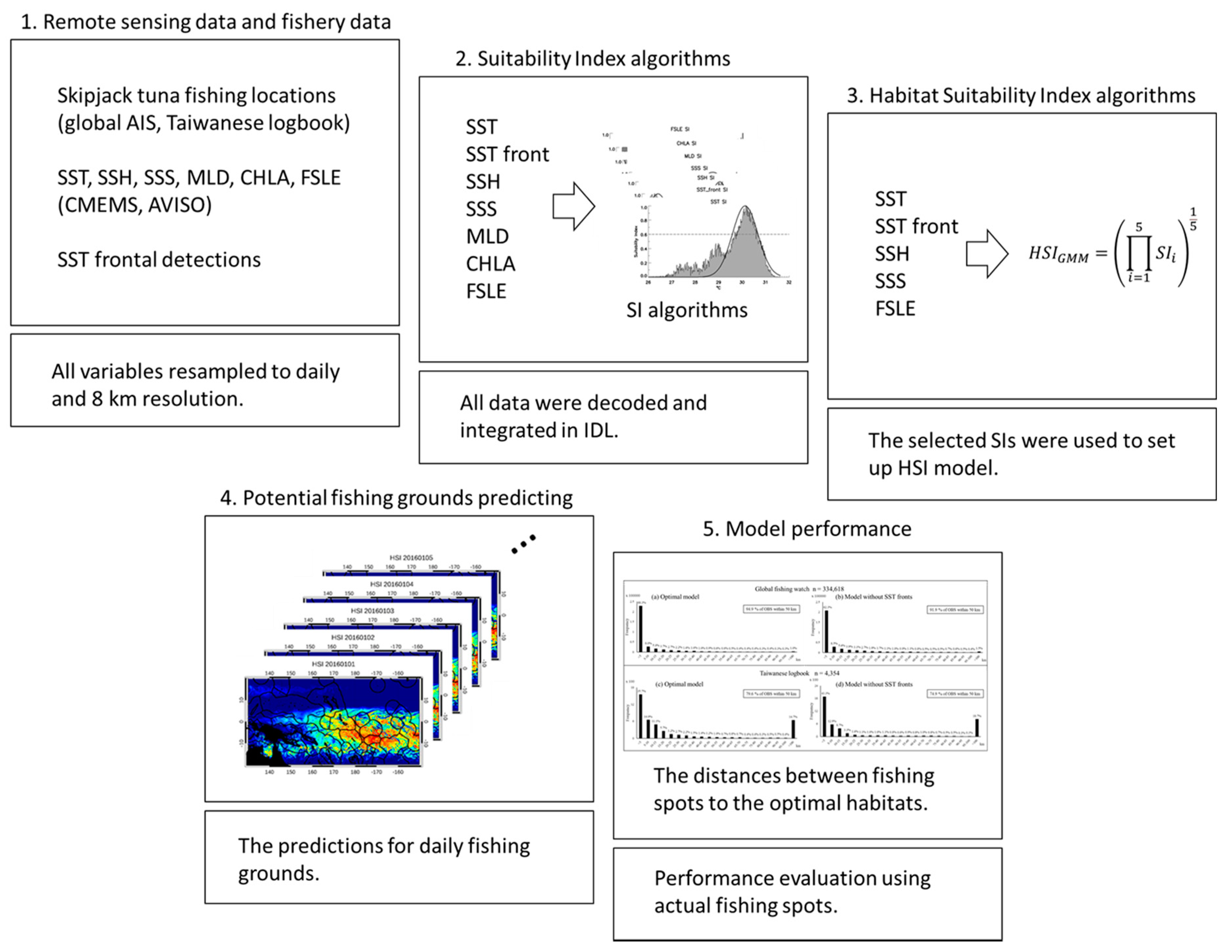
2. Materials and Methods

2.1. Skipjack Tuna Fishery Data

The traditional purse seine fishing areas of Taiwan are mainly distributed in the WCPO spanning from 130°E–150°W to 20°N–20°S, and all data were collected in this region (Figure 1). Two types of data were collected: Global datasets and Taiwan’s logbook data. Global datasets were obtained from Global Fishing Watch, which analyzed AIS data and identified fishing activities during the period from 2012 to 2016 [31]. The datasets contain fishing activities at 0.01° resolution, and vessel presence by flag state and fishing gear type Taiwanese data were gathered from the Overseas Fishery Development Council (OFDC) of Taiwan during the year of 2016. Logbook data comprised daily fishing positions (longitude and latitude in 0.01° spatial grid), the school type of fish, the set type of fishing, and the total catch (in tons). To facilitate the compilation of all data from inconsistent spatial scales, the original data were aggregated into the same grid resolution as environmental data.
Industrial tropical purse seiners deploy fish aggregating devices (FADs), which are known to provide geo-locations of objects to attract the target tuna [32,33]. Some FADs are powerful in not only locating valuable targets, but also highlight the signals of non-targets [34]. Hence, we used only free-swimming schools from Taiwan’s logbook data for further analysis.

2.2. Remotely-Sensed Environmental Data

The oceanographic variables (Table 1) used for modelling the habitat suitability index include sea surface temperature (SST) and its gradient (SST front; calculated as the peak and ridge temperature features in the same pixel) [35], sea surface salinity (SSS), sea surface height (SSH), mixed layer depth (MLD), chlorophyll a concentration (CHLA), and finite-size Lyapunov exponents (FSLE). Oceanic fronts are known for their characteristic of increased abundance and diversity of taxa ranging from phytoplankton to top predators [36]. The SST front detection algorithm is based on the gradient magnitude, which reveals the fine scale of boundaries between water masses (Figure 2). These operational variables were chosen because they are known to affect catches of tuna [2,19,37,38].
For the end user, the Copernicus Marine Environment Monitoring Service (CMEMS website provides level-4 products of daily mean SST, SSS, SSH, and MLD that were generated using a statistical model based on both satellite-derived data and in situ observations. CHLA concentration was derived as a weekly mean because of low coverage of cloud-free pixels in daily satellite-derived images (available at http://marine.copernicus.eu/ (accessed on 17 January 2021)). For the SST product, multiple satellites are integrated from the Advanced Very-High-Resolution Radiometer (AVHRR), Environmental Satellite (Envisat), Aqua, and the Tropical Rainfall Measuring Mission (TRMM). The SSS product is based on the data derived from the satellite Soil Moisture Ocean Salinity (SMOS) and in situ salinity measurements. SSH and MLD products are processed from all altimeter missions: Jason-3, Sentinel-3A, HaiYang-2A (HY-2A), Saral/AltiKa, Cryosat-2, Jason-2, Jason-1, TOPEX/Poseidon (T/P), ENVISAT, Geosat Follow-On (GFO), and European Remote Sensing Satellite 1/2 (ERS1/2). CHLA product is based on the merging of multiple sensors of the Sea-viewing Wide Field-of-view Sensor (SeaWiFS), Moderate Resolution Imaging Spectroradiometer (MODIS), Medium Resolution Imaging Spectrometer (MERIS), Visible Infrared Imaging Radiometer Suite (VIIRS), Suomi National Polar-orbiting Partnership (SNPP), and the Joint Polar-orbiting Satellite System-1 (JPSS1). The CMEMS products are available for 50 geopotential coverage levels from 0 to 5000 m. Due to the near-surface water fishing operation, the upper level (0 to 5 m) oceanographic factors were selected for model construction.
Daily mean FSLE data were download from Archiving Validation and Interpretation of Satellite Oceanographic (AVISO) data with a spatial resolution of 1/25 degree (~4 km) (available at https://www.aviso.altimetry.fr/ (accessed on 17 January 2021)). All datasets and SST frontal detections were decoded and integrated by code programming in Interactive Data Language (IDL 8.7.2) using the Advanced Math and Stats Module (IMSL). All environmental variables were resampled to 0.08-degree (~8 km) resolution on the basis of the coarsest scale.

2.3. Habitat Suitability Index Model

We started by fitting global datasets from 2012 to 2015 with remote sensing data to establish the HSI model. First, the suitability index (SI) was calculated using the frequency distribution of environmental parameters. The SI was described as a score, ranking from 0 to 1 for inappropriate and optimal habitats, respectively:
This is an example of the equation:
S I e n v = e ( α ( e n v + β ) ) 2
In Equation (1), α and β are the regression coefficients, which were modified by the least-squares method to assess the residuals between observations and functions of SI [21]. e n v is the value for each environmental parameter. After calculating the SI values, the SIs were subsequently developed to determine the overall habitat preference. We used the geometric mean model (GMM) to set up the HSI model [21,39].
The GMM model is described as follows:
H S I G M M = ( i = 1 n S I i ) 1 n
where n is the number of selected environmental parameters for setting up the HSI algorithm, and S I i is the SI for the i th environmental variable. Similar to the SI, the HSI has values ranging from 0 to 1.0, indicating not suitable to optimal, respectively [26,39]. HSI values equal to or higher than 0.6 were regarded as indicating potential fishing grounds [25].

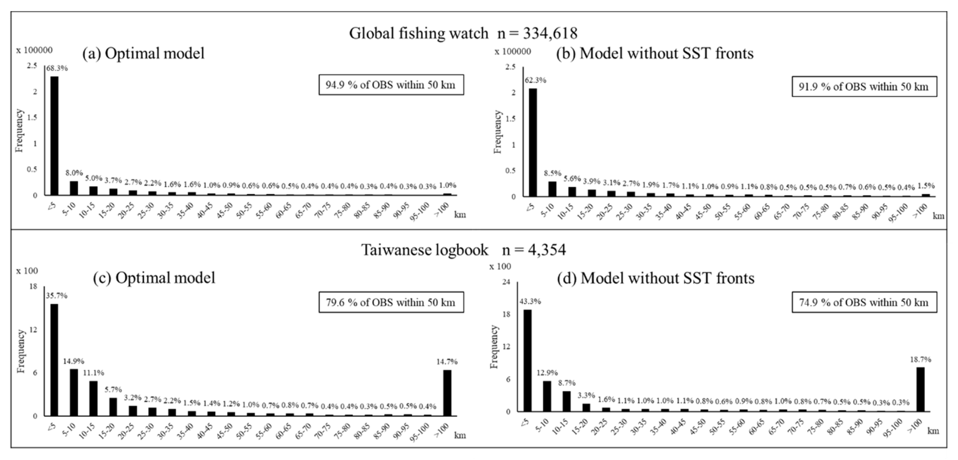
2.4. Calculation of Predicting Rate

To evaluate the model’s performance, we calculated the habitat suitability index using environmental data in the year of 2016 and compared it with untrained fishing activities data, included in global datasets and Taiwan’s logbook data over the same period, to estimate the fishing grounds of skipjack tuna in the WCPO.
The distance between the observed fishing effort and the boundary of potential fishing grounds derived from the HSI model is the clearest approach to show the ability of our model to locate potential fishing grounds. The accuracy rates were defined by the ratio of fishing activity occurring within different distances to the potential fishing grounds [11]. The workflow of this study is demonstrated in (Figure 3).

3. Results

3.1. Variations of Skipjack Tuna in the WCPO

The quarterly spatial distribution of fishing efforts from 2012 to 2015 at 1 degree resolution (Figure 4) showed quarterly variations. The global datasets are indicated in gray circles, which were widely distributed in the Pacific Ocean for all quarters. The Taiwanese vessels are shown by red dots and were mainly concentrated in the exclusive economic zone (EEZ) of Papua New Guinea, Nauru, Federated States of Micronesia, and west Kiribati (165°E–175°W and 5°N–5°S) and extended to Central Kiribati (170°W) in the second quarter. In 2016 (Figure 5), location variations were clearly seen in the third quarter. Global datasets showed less activity in the east high seas (170°W–160°W). Meanwhile, Taiwanese vessels (Figure 6) were concentrated in the EEZ of Nauru and Kiribati (165°E–180°E). Due to the lack of logistic lines and supplemental ports, Taiwanese purse seine vessels did not tend to fish on the east side of the Pacific Ocean from the commercial profit perspective.

3.2. Suitability Index Analysis and Habitat Suitability Index Model

The intention for model development based on environmental variables and fishery data was to classify the preferred regions for skipjack tuna from a remote sensing perspective. A total of 737,167 datapoints were used in the HSI model, taken from the global datasets in the period of 2012–2015. The suitability index equations for each parameter, derived from global datasets, are shown in Table 2. All environmental parameters were analyzed for statistical significance. For purse seiners, the optimal range (SI ≧ 0.6) of skipjack tuna was defined as a slightly hotter SST, higher than 29.6 °C (Figure 7a), an SST front of approximately 0.01–0.11 °C/km (Figure 7b), an SSH of approximately 0.60–0.71 m (Figure 7c), an SSS of approximately 34.29–35.28 PSU (Figure 7d), an MLD shallower than 10.81 m (Figure 7e), a CHLA of approximately 0.03–0.04 mg/m3 (Figure 7f), and an FSLE greater than −0.05 day−1 (Figure 7g). Furthermore, the optimal ranges of SST, SST front, SSH, SSS, and FSLE accounted for 60.00%, 62.66%, 51.26%, 57.40%, and 64.50% of total efforts, respectively (Table 2).
The daily distributions of operation locations from the 20 to 23 August 2016, with SST and SST front images are shown in Figure 8. The fishing spots were mainly distributed in Nauru and Kiribati waters, where the adjacent water masses on the east side are cold and on the west side are warm. The fishing spots were in warm water where the SST was higher than 29 °C and there was a low gradient of SST front (Figure 8, left column). Furthermore, the high-gradient SST front was more associated with fishing grounds. The strong SST front did not specifically appear in the fishing datasets; nevertheless, the fishing grounds were not far from strong fronts (Figure 8, right column).

3.3. Accuracy of the HSI Model

Five suitable ranges of environmental variables, which accounted for up to 50% of total efforts, were used, i.e., SST, SST front, SSH, SSS, and FSLE (Table 2). These were selected to derive the HSI model for skipjack tuna. The period of 2016 was chosen to calculate the accuracy of the HSI model by comparing data with fishery efforts, including global datasets and Taiwanese logbook data. In the overview of 2016, 68.3% of global data was within 5 km of suitable areas, whereas 94.9% were within 50 km (Figure 9a). In contrast, 35.7% of Taiwanese logbook data occurred within 5 km, and 79.6% were found within 50 km of suitable areas (Figure 9c). The accuracy of the model without SST fronts was compared, and found to decrease to 62.3% and 91.9% within 5 and 50 km, respectively, in global data (Figure 9b). Taiwanese logbook data showed increased accuracy (43.3%) in the area within 5 km but lower accuracy of 74.9% within 50 km (Figure 9d). As a consequence, SST fronts is the parameter which improves the predictability of fishing grounds in the suitability index-based models.

3.4. The Outputs of the HSI Model and Purse Seine Fishing

The outputs of the habitat model in 2016 are shown in Figure 5, and global datasets showed that fishing activities generally occurred in the equatorial region, except for the Phoenix Islands Protected Area (175°W–170°W). The fishing hours decreased in the high seas (170°W–160°W) from quarter 1 and were nearly absent in quarter 3. Notable, in the Central Pacific, Nauru and West Kiribati are two important fishing grounds for purse seiners, showing long fishing hours throughout the year. The habitat derived from the HSI model shifted northwest to the Federated States of Micronesia and Papua New Guinea in quarter 2, and continued to quarter 4. Simultaneously, the length of fishing hours showed the same trend, moving northwest and extending to the south of the EEZ in the Federated States of Micronesia. In general, the suitable habitat displayed a large horizontal shift in the period of quarters 1 and 2, but was relatively stable in quarter 2–quarter 4. In comparison, Taiwanese purse seine vessels showed less variations in the vertical and horizontal directions (Figure 6). In quarter 1, fishing efforts mainly occurred in the EEZ of Nauru, the junction (4°S) of west Kiribati and Tuvalu, Solomon Islands. The high seas (178°W–176°W) between Tuvalu and central Kiribati also showed dense fishing activities. In quarter 2, fishing locations shifted northward and westward, similar to the shift in suitable habitat. Skipjack tuna were caught across the EEZ of Papua New Guinea and along the line from Federated States of Micronesia to Marshall Islands. In quarter 3, fewer suitable habitats were detected in Tuvalu, Tokelau, and Cook Islands, whereas the Western Pacific was highlighted as a suitable fishing ground. The catches were also mainly concentrated in two areas: the central area between two high seas (151°E–158°E) and the EEZ of Nauru to Central Kiribati. Suitable habitats were no longer present in the Western Pacific in quarter 4. Instead, the HSI model marked the south edge of the EEZ of Nauru, the north of the Federated States of Micronesia, and all of Tokelau, as suitable habitats. Catches were concentrated on the south side of Nauru and north side of Papua New Guinea, and were sporadic between Pohnpei and Majuro.
Overall, in both datasets, the EEZs of Nauru and Kiribati were the most popular fishing areas (163°E–180°E, 2°N–3°S), except in quarter 2. The east high seas surrounding Kiribati (167°W–160°W) were marked as a suitable habitat in quarters 1 and 2, and the fishing activities in the global dataset presented the same spatial distribution for the same period, but Taiwanese vessels were absent in this region. Taiwanese vessels appeared to avoid crossing the vertical line of 180°E, showing few records in the narrow high seas. An increase in fishing activities was also found in both datasets: the recorded number fishing activities in both datasets in the study area increased by 1.5 times from quarter 1 to 4. Taiwanese and global datasets recorded the highest fishing activities in quarters 3 and 4, respectively.

4. Discussion

The HSI model theory led us to infer characteristics of the skipjack tuna habitat in the WCPO and build a forecasting system using fishery and satellite remote sensing data to locate potential fishing grounds. The fishery data collected were not field survey quality because fishing masters determined fishing locations according to their own choice and not by random selection. However, fishery data are easy to acquire, and low-cost species survey data sets are available to scientists [2]. Here we obtained fishing effort data that covered a wide geographical area, and data were from all operational purse seine vessels in the WCPO. The advantage of using remote sensing data is the efficiency in measuring parameters on the oceanic scale compared to on-site investigations [40]. By programming code, we were able to construct an automatic procedure to locate interesting areas for finding target fish in just a few minutes.
The global purse seine fishery industry operates in the Pacific Ocean over a wide distribution from 140°E to 150°W. In contrast, traditional fishing grounds for Taiwanese vessels mainly occurred around the Federated States of Micronesia, Papua New Guinea, Solomon Islands, and Kiribati from 1997 [41]. Skipjack tuna follow a brief route to the south for spawning and retreat to the north during the summer [42]. Fishing efforts extended south to the Solomon Islands in quarters 1 and 4, and they withdrew from the south in quarters 2 and 3 in both datasets (Figure 4, Figure 5 and Figure 6). These shifts seem to reflect the migration route of skipjack tuna following the south–north pathway. The high sea pocket was enclosed from 1 January 2010 for conservation management [43]. The footprints of Taiwanese purse seines were present around the high sea pocket (i.e., they were fishing-the-line), and the fishing masters obtained benefits from the spillover of the enclosed area (Figure 4).
Typically, the western Pacific is a warm pool with an annual maximum sea surface temperature of 30 °C, and a higher density of skipjack tuna gather there [22,23]. The SST in this study was slightly higher compared to previous studies, ranging from 20.5 to 26.0 °C for skipjack in the Western North Pacific Ocean [2] and over 24 °C in the Western Pacific Ocean [1]. A possible explanation for this might be the sampling bias derived from the tendency for operational fleets to find targets in higher SSTs. Another possible explanation is a regional bias derived from the different resource types of data and collecting areas. There are, however, other possible explanations. It is thought that predators (tuna) cluster around the front area where the prey is located [44], and thermal fronts are also associated with a high probability of the skipjack population [17].
The findings of the SST front were confirmed in the lower gradient change from 0.01 to 0.11 °C/km. The most likely cause of this lower gradient change is that fishing spots are located at the junction of the convergence zone of the warm pool and the tongue of cold surface water [23]. The cold tongue is nutrient-enriched, which benefits prey, and the warm pool offers a place for skipjack tuna to cluster. Skipjack tuna move to cooler water for ingestion and swim into warm water due to its comfortable temperature. The fishing activities of skipjack tuna occur in warm water, near the convergence zone of warm and cold water where there is less gradient change compared to the junction of two water masses. Our findings indicate that the actual fishing grounds were closely associated with adjacent areas of strong SST fronts rather than in the center of strong fronts (Figure 8).
A higher value of SSH influences the suitable range of skipjack tuna, and this was confirmed in our study. For example, SSH ranged from 0 to 50 cm in the Western North Pacific Ocean [2], and 70–100 cm in the WCPO [14,15], which were defined by the generalized additive model (GAM) method, and 80–90 cm by the empirical cumulative distribution function in Sri Lankan waters [13]. The intermediate values of these findings coincided with our results ranging from 60 to 71 cm (Figure 7c), given that the datasets in our study had broad coverage. The salinity broadly ranges from 33.0 to 37.2 PSU for the world oceans [16]; 5th and 95th percentile values ranged from 34.9 to 35.8 PSU in the Southwestern Atlantic according to the GAM method [17], and 30.3 to 36.2 PSU was recorded in the Eastern central Atlantic and Western Indian Oceans by the ecological niche model [10]. High salinity values above 35.8 PSU present oligotrophic conditions and lower primary productivity, which cannot support feeding requirements for skipjack tuna in tropical waters [17]. A suitable range from 34.29 to 35.28 PSU (Figure 7d) was seen under the border limit and is consistent with previous studies.
Skipjack tuna do not resist hypoxic water where there is less than 3.5 mL O2 per liter [16], and this restricts skipjack tuna to inhabit the mixed layer above the thermocline [2]. The MLD from 6 to 158 m was confirmed as a favorable feeding habitat for skipjack [11]. A fishing master works towards better sinking performance, where faster and greater sinking depth means a higher probability of a successful set [45]. Underwater nets are attached to FADs; the length can reach a depth of 50 m [46], and the common average depth is 15–20 m [33]. Moreover, MLD associated with oxygen restriction affects the vertical distribution of tuna, and larger skipjacks with greater requirements are more spatially confined [9]. The suitable range of MLD reflects the selection of fishing operations more than the suitability of the skipjack tuna habitat. In our findings, the suitable range of MLD showed a highly left-skewed distribution (Figure 7e) and accounted for 20% of total efforts (Table 2). We propose that the MLD, which implies the limit of oxygen concentration, does not directly reflect fishing activities.
Chlorophyll concentration has direct or indirect relationships with the foraging distribution, and affects the predators [2]. The specific value of 0.2 mg/m3 was described as an indicator for the highest CPUE and fishing frequency in the gulf of the Bone-Flores Sea, Indonesia [12]. A similar range of 0.1 to 0.3 mg/m3 was also shown in the Western North Pacific [2]. A widely defined favorable range between 0.13 and 5.27 mg/m3 exists in the Atlantic and Indian Oceans [11]. Furthermore, fishing positions in the aforementioned studies were mostly located in coastal areas known for high nutrient concentrations. There is a discrepancy between our findings ranging from 0.03 to 0.04 mg/m3 (Figure 7f) and a previous study on the suitable range of CHLA. We assumed this difference resulted from feeding habits. As a piscivorous feeder, skipjack tuna also depends on various prey [47]. Skipjack tuna can easily adapt their survival strategy to the local prey composition [47,48], different food consumptions of tuna between FAD-associated and -unassociated schools [49], and feeding habit variations in different current systems [47]. Thus, the feeding strategy in distant waters with poorer nutritional conditions seems to differ from the relatively high CHLA region.
Unlike other physical oceanic parameters, the FSLE is new dynamic concept developed using the Lagrangian technique. This new concept crucially influences the marine top predators, indicating their foraging behavior, movement distribution, etc. [18,19,20]. For example, strong Lagrangian fronts imply a zooplankton concentration and larger quantities of fish, and more prey, in the Southern Indian Ocean [18]. Tuna fishermen track strong Lagrangian coherent structures where three times more profits per trip are expected in the U.S. in California [20]. A strong FSLE represents an area of aggregated fish, but this strong oceanic dynamic also represents stirring and strongly organizes the fluid motion. The prerequisites for successful purse seine fishing operations are the direction and speed of the wind and current [50], which are strong under current due to the shear force, and this may cause damage to the net. FSLE ranges close to zero (Figure 7g) indicate better conditions for purse seine fishing, although they may not represent the highest density of skipjack tuna.
After determining the optimal range for each environmental parameter relevant to skipjack tuna from global datasets, the accuracy of the HSI model was determined (Figure 7). HSI values in the accumulation map were appreciably concurrent with fishing spots for 2016 (Figure 5). The present model appears to have defects in describing the spatial distribution in the first quarter (Figure 5 and Figure 6); the HSI values were highly accumulated in Tokelau and Cook Islands waters. Meanwhile, the actual fishing spots were mainly distributed in the region on the west side of the Pacific Ocean, for either global or Taiwanese data. The major distant water fishing nations, which include Korea (15%), Japan (14%), Taiwan (12%), and the USA (11%), accounted for all of the WCPO tuna catches by weight [51]. This list of major nations mostly comprises Asian nations. Considering multiple essential factors, such as increased supply line costs and oil prices, it is not difficult to imagine that Asian nations tend to fish on the western side of the Pacific. Even if most of the fish were on the east side of the Pacific, fishing vessels still fish in adjacent areas rather than chasing distant targets. Furthermore, fishing is moving toward FAD-based strategies instead of free-swimming school sets. In addition, the advantages of FADs are shown in three important aspects: the high success rates, stable schooling situations, and higher average catch [52]. Distinguishable behaviors of skipjack tuna include moving over long distances or their association with floating objects in the El Niño-Southern Oscillation (ENSO) [53]. Purse seine vessels no longer chase free-swimming schools, and powerful multifunction buoys are the first choice. Most FAD sets are done in the early morning, before sunrise, and most can still search for free-swimming schools during the day [46]. Therefore, it can be concluded that the FAD and the associated cost showed changes in fishing activity patterns and moving strategies.
In Taiwanese logbook data, about 20% of free-swimming sets were far from the optimal habitat boundary (>50 km), whereas the global data represented 5% of all sets, suggesting that the model performed well in fitting daily forecasting habitats and actual fishing position. However, quarterly accumulation of HSI appears to coincide with defects in quarter 1 (Figure 5).

5. Conclusions

This study successfully developed an HSI model, which could be an efficient tool to forecast potential fishing grounds because it projects optimal habitat selection for skipjack tuna using fishery data and environmental parameters from a high spatial–temporal resolution and remote sensing perspective. Our automatic process could be ideally used to assist in management scenarios, to avoid marine protected areas, and to ensure proper areas are fished and eco-friendly regulations are followed. The dominant fishing grounds were not far from areas of strong SST fronts. Moreover, the model without SST fronts was compared with the optimal model to examine how SST fronts can improve the predictability of fishing grounds in the HSI model. Overall, the accuracies of the two datasets generally declined in the model without SST fronts. The decrease in SI elements (from 5 SI to 4 SI) implies a looser filter for determining suitable habitat. The model without SST fronts did not benefit from a loose filter to obtain higher accuracy compared with the optimal model. The result shows that SST fronts can improve the predictability of fishing grounds.
Future work should expand on our algorithm to improve the forecasting rate and provide precise directions of optimal fishing areas. In addition, considering more oceanic parameters, such as dissolved oxygen [9], could be helpful in detailing the habitat suitability index for skipjack tuna, in addition to identifying both fishing and weather conditions to determine optimal fishing conditions and fish locations.

Author Contributions

All authors contributed to this study; conceptualization and methodology. T.-Y.H. constructed the code for processing and analyzing data and wrote the original draft manuscript; Y.C. and S.-C.H. reviewed and edited the draft manuscript, M.-A.L. and R.-F.W. contributed data of Taiwanese purse seine fisheries. All authors have read and agreed to the published version of the manuscript.

Funding

This research was funded by the National Science Council (MOST 107-2611-M-006-003), and Council of Agriculture (108AS-9.1.4-FA-F1(5)).

Institutional Review Board Statement

Not applicable.

Informed Consent Statement

Not applicable.

Data Availability Statement

GFW data used in this study are available from (www.globalfishingwatch.org (accessed on 17 January 2021)).

Acknowledgments

The authors are grateful to the Overseas Fishery Development Council of Taiwan and the Fisheries Agency for providing data from the Taiwanese purse seine distance fishery and Global Fishing Watch for the GFW website. We acknowledge the use of oceanic parameter data from the Copernicus Marine Environment Monitoring Service, the FSLE data distributed by AVISO.

Conflicts of Interest

The authors declare no conflict of interest.

References

  1. Ashida, H. Spatial and temporal differences in the reproductive traits of skipjack tuna Katsuwonus pelamis between the subtropical and temperate western Pacific Ocean. Fish. Res. 2020, 221. [Google Scholar] [CrossRef]
  2. Mugo, R.; Saitoh, S.-I.; Nihira, A.; Kuroyama, T. Habitat characteristics of skipjack tuna (Katsuwonus pelamis) in the western North Pacific: A remote sensing perspective. Fish. Oceanogr. 2010, 19, 382–396. [Google Scholar] [CrossRef]
  3. Miyabe, N.; Nakano, H. Historical Trends of Tuna Catches in the World; Food & Agriculture Org.: Rome, Italy, 2004. [Google Scholar]
  4. Langley, A.; Hampton, J.; Ogura, M. Stock Assessment of Skipjack Tuna in the Western and Central Pacific Ocean; WCPFC SC1 SA WP-4, 69 pp. Bigeye Tuna Yellowfin Tuna 2005; WCPFC: Kolonia, Federated States of Micronesia, 2005. [Google Scholar]
  5. Miyake, M.P.; Guillotreau, P.; Sun, C.-H.; Ishimura, G. Recent Developments in the Tuna Industry: Stocks, Fisheries, Management, Processing, Trade and Markets; Food and Agriculture Organization of the United Nations: Rome, Italy, 2010. [Google Scholar]
  6. FAO. FAO Yearbook: Fishery and Aquaculture Statistics; FAO: Rome, Italy, 2017. [Google Scholar]
  7. WCPFC. Tuna Fishery Yearbook 2017; Western Central Pacific Fisheries Commission: Kolonia, Federated States of Micronesia, 2018. [Google Scholar]
  8. Lehodey, P.; Bertignac, M.; Hampton, J.; Lewis, A.; Picaut, J. El Niño Southern Oscillation and tuna in the western Pacific. Nature 1997, 389, 715–718. [Google Scholar] [CrossRef]
  9. Graham, J.B.; Dickson, K.A. Tuna comparative physiology. J. Exp. Biol. 2004, 207, 4015–4024. [Google Scholar] [CrossRef] [PubMed] [Green Version]
  10. Druon, J.; Chassot, E.; Murua, H.; Soto, M. Preferred feeding habitat of skipjack tuna in the eastern central Atlantic and western Indian Oceans: Relations with carrying capacity and vulnerability to purse seine fishing. In Proceedings of the Scientific Committee of the Indian Ocean Tuna Commission-working Party on Tropical Tunas, Mahe, Seychelles, 5–10 November 2016. [Google Scholar]
  11. Druon, J.-N.; Chassot, E.; Murua, H.; Lopez, J. Skipjack Tuna Availability for Purse Seine Fisheries Is Driven by Suitable Feeding Habitat Dynamics in the Atlantic and Indian Oceans. Front. Mar. Sci. 2017, 4. [Google Scholar] [CrossRef]
  12. Zainuddin, M.; Farhum, A.; Safruddin, S.; Selamat, M.B.; Sudirman, S.; Nurdin, N.; Syamsuddin, M.; Ridwan, M.; Saitoh, S.I. Detection of pelagic habitat hotspots for skipjack tuna in the Gulf of Bone-Flores Sea, southwestern Coral Triangle tuna, Indonesia. PLoS ONE 2017, 12, e0185601. [Google Scholar] [CrossRef] [PubMed] [Green Version]
  13. Rathnasuriya, M.I.G. Environmental Effect on the Skipjack Tuna (Katsuwonus pelamis) Fishery in the Sri Lankan Waters; Pukyong National University: Busan, Korea, 2016. [Google Scholar]
  14. Tang, H.; Xu, L.-X.; Chen, X.-J.; Zhu, G.-P.; Zhou, C.; Wang, X.-F. Effects of spatiotemporal and environmental factors on the fishing ground of Skipjack Tuna (Katsuwonus pelamis) in the western and central Pacific Ocean based on generalized additive model. Mar. Environ. Sci. 2013, 32, 518–522. [Google Scholar]
  15. Wang, J.; Chen, X.; Chen, Y. Spatio-temporal distribution of skipjack in relation to oceanographic conditions in the west-central Pacific Ocean. Int. J. Remote Sens. 2016, 37, 6149–6164. [Google Scholar] [CrossRef]
  16. Arrizabalaga, H.; Dufour, F.; Kell, L.; Merino, G.; Ibaibarriaga, L.; Chust, G.; Irigoien, X.; Santiago, J.; Murua, H.; Fraile, I.; et al. Global habitat preferences of commercially valuable tuna. Deep Sea Res. Part Ii Top. Stud. Oceanogr. 2015, 113, 102–112. [Google Scholar] [CrossRef] [Green Version]
  17. Coletto, J.L.; Pinho, M.P.; Madureira, L.S.P. Operational oceanography applied to skipjack tuna (Katsuwonus pelamis) habitat monitoring and fishing in south-western Atlantic. Fish. Oceanogr. 2018, 28, 82–93. [Google Scholar] [CrossRef] [Green Version]
  18. Baudena, A.; Ser-Giacomi, E.; d’Onofrio, D.; Capet, X.; Cotté, C.; Cherel, Y.; d’Ovidio, F. Fine-scale fronts as hotspots of fish aggregation in the open ocean. bioRxiv 2019. [Google Scholar] [CrossRef]
  19. Kai, E.T.; Rossi, V.; Sudre, J.; Weimerskirch, H.; Lopez, C.; Hernandez-Garcia, E.; Marsac, F.; Garçon, V. Top marine predators track Lagrangian coherent structures. Proc. Natl. Acad. Sci. USA 2009, 106, 8245–8250. [Google Scholar]
  20. Watson, J.R.; Fuller, E.C.; Castruccio, F.S.; Samhouri, J.F. Fishermen Follow Fine-Scale Physical Ocean Features for Finance. Front. Mar. Sci. 2018, 5. [Google Scholar] [CrossRef]
  21. Yen, K.-W.; Lu, H.-J.; Chang, Y.; Lee, M.-A. Using remote-sensing data to detect habitat suitability for yellowfin tuna in the Western and Central Pacific Ocean. Int. J. Remote Sens. 2012, 33, 7507–7522. [Google Scholar] [CrossRef]
  22. Lan, K.-W.; Shimada, T.; Lee, M.-A.; Su, N.-J.; Chang, Y. Using Remote-Sensing Environmental and Fishery Data to Map Potential Yellowfin Tuna Habitats in the Tropical Pacific Ocean. Remote Sens. 2017, 9, 444. [Google Scholar] [CrossRef] [Green Version]
  23. Receveur, A.; Nicol, S.; Tremblay-Boyer, L.; Menkes, C.; Senina, I.; Lehodey, P. Using SEAPODYM to better understand the influence of El Niño Southern Oscillation on Pacific tuna fisheries. Spc Fish. Newsl. 2016, 149, 31–36. [Google Scholar]
  24. Brooks, R.P. Improving habitat suitability index models. Wildl. Soc. Bull. (1973–2006) 1997, 25, 163–167. [Google Scholar]
  25. Lee, M.-A.; Weng, J.-S.; Lan, K.-W.; Vayghan, A.H.; Wang, Y.-C.; Chan, J.-W. Empirical habitat suitability model for immature albacore tuna in the North Pacific Ocean obtained using multisatellite remote sensing data. Int. J. Remote Sens. 2019. [Google Scholar] [CrossRef]
  26. Uenaka, T.; Sakamoto, N.; Koyamada, K. Visual Analysis of Habitat Suitability Index Model for Predicting the Locations of Fishing Grounds. In Proceedings of the 2014 IEEE Pacific Visualization Symposium, Yokohama, Japan, 4–7 March 2014; pp. 306–310. [Google Scholar]
  27. Stelzenmüller, V.; Ehrich, S.; Zauke, G.-P. Effects of survey scale and water depth on the assessment of spatial distribution patterns of selected fish in the northern North Sea showing different levels of aggregation. Mar. Biol. Res. 2005, 1, 375–387. [Google Scholar] [CrossRef]
  28. Bordalo-Machado, P. Fishing Effort Analysis and Its Potential to Evaluate Stock Size. Rev. Fish. Sci. 2007, 14, 369–393. [Google Scholar] [CrossRef]
  29. Abernethy, K.E.; Allison, E.H.; Molloy, P.P.; Côté, I.M. Why do fishers fish where they fish? Using the ideal free distribution to understand the behaviour of artisanal reef fishers. Can. J. Fish. Aquat. Sci. 2007, 64, 1595–1604. [Google Scholar] [CrossRef]
  30. Swain, D.P.; Wade, E.J. Spatial distribution of catch and effort in a fishery for snow crab (Chionoecetes opilio): Tests of predictions of the ideal free distribution. Can. J. Fish. Aquat. Sci. 2003, 60, 897–909. [Google Scholar] [CrossRef]
  31. Global Fishing Watch. Available online: www.globalfishingwatch.org (accessed on 17 January 2021).
  32. Dagorn, L.; Holland, K.N.; Restrepo, V.; Moreno, G. Is it good or bad to fish with FADs? What are the real impacts of the use of drifting FADs on pelagic marine ecosystems? Fish Fish. 2013, 14, 391–415. [Google Scholar] [CrossRef]
  33. Orue, B.; Lopez, J.; Moreno, G.; Santiago, J.; Soto, M.; Murua, H. Aggregation process of drifting fish aggregating devices (DFADs) in the Western Indian Ocean: Who arrives first, tuna or non-tuna species? PLoS ONE 2019, 14, e0210435. [Google Scholar] [CrossRef] [Green Version]
  34. Boyra, G.; Moreno, G.; Sobradillo, B.; Pérez-Arjona, I.; Sancristobal, I.; Demer, D.A.; Ratilal, P. Target strength of skipjack tuna (Katsuwanus pelamis) associated with fish aggregating devices (FADs). ICES J. Mar. Sci. 2018, 75, 1790–1802. [Google Scholar] [CrossRef]
  35. Belkin, I.M.; O’Reilly, J.E. An algorithm for oceanic front detection in chlorophyll and SST satellite imagery. J. Mar. Syst. 2009, 78, 319–326. [Google Scholar] [CrossRef]
  36. Woodson, C.; McManus, M.; Tyburczy, J.; Barth, J.; Washburn, L.; Caselle, J.; Carr, M.; Malone, D.; Raimondi, P.; Menge, B. Coastal fronts set recruitment and connectivity patterns across multiple taxa. Limnol. Oceanogr. 2012, 57, 582–596. [Google Scholar] [CrossRef] [Green Version]
  37. Kiyofuji, H.; Aoki, Y.; Kinoshita, J.; Okamoto, S.; Masujima, M.; Matsumoto, T.; Fujioka, K.; Ogata, R.; Nakao, T.; Sugimoto, N.; et al. Northward migration dynamics of skipjack tuna (Katsuwonus pelamis) associated with the lower thermal limit in the western Pacific Ocean. Prog. Oceanogr. 2019, 175, 55–67. [Google Scholar] [CrossRef]
  38. Matear, R.J.; Chamberlain, M.A.; Sun, C.; Feng, M. Climate change projection for the western tropical Pacific Ocean using a high-resolution ocean model: Implications for tuna fisheries. Deep Sea Res. Part Ii Top. Stud. Oceanogr. 2015, 113, 22–46. [Google Scholar] [CrossRef]
  39. Lauver, C.L.; Busby, W.H.; Whistler, J.L. Testing a GIS model of habitat suitability for a declining grassland bird. Environ. Manag. 2002, 30, 88–97. [Google Scholar] [CrossRef]
  40. Santos, A.M.P. Fisheries oceanography using satellite and airborne remote sensing methods: A review. Fish. Res. 2000, 49, 1–20. [Google Scholar] [CrossRef]
  41. Chang, S.-K.; Lu, H.-J. Taiwan tuna fisheries in the western-central Pacific Ocean, 1997. Presented at the Eleventh Meeting of the Standing Committee on Tuna and Billfish, Honolulu, HI, USA, 30 May–6 June 1998. [Google Scholar]
  42. Matsumoto, W.M. The Skipjack Tuna, Katsuwonus pelamis. Mar. Fish. Rev. 1974, 36, 26. [Google Scholar]
  43. WCPFC. Conservation and Management Measure for Bigeye and Yellowfin Tuna in the Western and Central Pacific Ocean; CMM 2008-01; WCPFC: Kolonia, Federated States of Micronesia, 2008. [Google Scholar]
  44. Lan, K.-W.; Kawamura, H.; Lee, M.-A.; Lu, H.-J.; Shimada, T.; Hosoda, K.; Sakaida, F. Relationship between albacore (Thunnus alalunga) fishing grounds in the Indian Ocean and the thermal environment revealed by cloud-free microwave sea surface temperature. Fish. Res. 2012, 113, 1–7. [Google Scholar] [CrossRef]
  45. Tang, H.; Xu, L.; Zhou, C.; Wang, X.; Zhu, G.; Hu, F. The effect of environmental variables, gear design and operational parameters on sinking performance of tuna purse seine setting on free-swimming schools. Fish. Res. 2017, 196, 151–159. [Google Scholar] [CrossRef]
  46. Fonteneau, A.; Pallares, P.; Pianet, R. A worldwide review of purse seine fisheries on FADs. In Proceedings of the Pêche Thonière et Dispositifs de Concentration de Poissons, Caribbean, Martinique, 15–19 October 1999. [Google Scholar]
  47. Tanabe, T. Feeding habits of skipjack tuna Katsuwonus pelamis and other tuna Thunnus spp. juveniles in the tropical western Pacific. Fish. Sci. 2001, 67, 563–570. [Google Scholar] [CrossRef]
  48. Varela, J.L.; Canavate, J.P.; Medina, A.; Mourente, G. Inter-regional variation in feeding patterns of skipjack tuna (Katsuwonus pelamis) inferred from stomach content, stable isotope and fatty acid analyses. Mar. Environ. Res. 2019, 152, 104821. [Google Scholar] [CrossRef]
  49. Ménard, F.; Stéquert, B.; Rubin, A.; Herrera, M.; Marchal, É. Food consumption of tuna in the Equatorial Atlantic Ocean: FAD-associated versus unassociated schools. Aquat. Living Resour. 2000, 13, 233–240. [Google Scholar] [CrossRef]
  50. Pravin, P. Purse Seine and its Operation; Central Institute of Fisheries Technology: Kerala, India, 2002. [Google Scholar]
  51. Liao, C.-P.; Huang, H.-W. The cooperation strategies of fisheries between Taiwanese purse seiners and Pacific Island Countries. Mar. Policy 2016, 66, 67–74. [Google Scholar] [CrossRef]
  52. Fonteneau, A.; Chassot, E.; Bodin, N. Global spatio-temporal patterns in tropical tuna purse seine fisheries on drifting fish aggregating devices (DFADs): Taking a historical perspective to inform current challenges. Aquat. Living Resour. 2013, 26, 37–48. [Google Scholar] [CrossRef] [Green Version]
  53. Wang, X.; Chen, Y.; Truesdell, S.; Xu, L.; Cao, J.; Guan, W. The large-scale deployment of fish aggregation devices alters environmentally-based migratory behavior of skipjack tuna in the Western Pacific Ocean. PLoS ONE 2014, 9, e98226. [Google Scholar] [CrossRef] [Green Version]
Figure 1. Map of the study area including the boundary of exclusive economic zones (EEZ) of each coastal state in the Western and Central Pacific Ocean.
Remotesensing 13 00861 g001
Figure 2. Examples of SST front detection (top row: 1 April 2016; bottom row: 1 September 2016). Left column (a,c), original SST images. Right column (b,d), gradient images.
Remotesensing 13 00861 g002
Figure 3. An illustration of workflow implemented for this study. The numbers are the step by step order.
Remotesensing 13 00861 g003
Figure 4. Quarterly distributions of 1° × 1° grid (global datasets: Gray circles; Taiwanese datasets: Red dot) during the years 2012–2015. Black contour lines are exclusive economic zones.
Remotesensing 13 00861 g004
Figure 5. Fishing hours of global datasets of 1° spatial grid with habitat variation. The quarterly habitat is defined by the presence of habitat suitability index (HSI) values and shows the occurrence accumulation: (a) quarter 1, (b) quarter 2, (c) quarter 3, and (d) quarter 4 in 2016.
Remotesensing 13 00861 g005
Figure 6. Fishing spots of Taiwanese operational vessels with habitat variation: (a) quarter 1, (b) quarter 2, (c) quarter 3, and (d) quarter 4 in 2016.
Remotesensing 13 00861 g006
Figure 7. Suitability index curve for environmental variables: (a) SST, (b) SST front, (c) SSH, (d) SSS, (e) MLD, (f) CHLA, and (g) FSLE. The gray bars, solid curve lines, and dotted lines show the SI values, fitted SI curves, and 0.6 intervals (good habitat), respectively.
Remotesensing 13 00861 g007
Figure 8. Spatial distribution of skipjack tuna fishing locations (global and Taiwanese data, gray and red circles, respectively) overlaid on daily (ad) SST and (eh) SST front images in the period of 20–23 August 2016. The SST fronts below 0.5 are transparent to emphasize the strong fronts.
Remotesensing 13 00861 g008
Figure 9. Histograms of the distances observed between fishing locations to the closet habitat boundary derived from (a) global datasets and (c) Taiwanese datasets in 2016; (b) global and (d) Taiwanese datasets in the model without SST fronts.
Remotesensing 13 00861 g009
Table 1. List of satellite remote sensing data and the data sources.
ParametersData SourceUnitSpatial ResolutionTemporal Resolution
Sea Surface Temperature (SST)https://marine.copernicus.eu/ (accessed on 17 January 2021)°C8 × 8 kmdaily
Sea Surface Temperature frontdetected from SST°C/km8 × 8 kmdaily
Sea Surface Height (SSH)https://marine.copernicus.eu/ (accessed on 17 January 2021)m8 × 8 kmdaily
Sea Surface Salinity (SSS)https://marine.copernicus.eu/ (accessed on 17 January 2021)PSU8 × 8 kmdaily
Mixed Layer Depth (MLD)https://marine.copernicus.eu/ (accessed on 17 January 2021)m8 × 8 kmdaily
Chlorophyll a concentration (CHLA)https://marine.copernicus.eu/ (accessed on 17 January 2021)mg/m38 × 8 kmweekly
Finite-Size Lyapunov Exponents (FSLE)https://www.aviso.altimetry.fr/ (accessed on 17 January 2021)day−14 × 4 kmdaily
Table 2. The equations of suitability index (SI) derived from environmental variables.
VariableSI ModelsF Valuep ValueAccounted Rate of Total Efforts
(SI Value ≧ 0.6)
SST exp ( 1.69 ( X S S T 30.13 ) 2 ) 2628.26<0.0160.00%
SST front exp ( 207.43 ( X s s t f t 0.06 ) 2 ) 4374.82<0.0162.66%
SSH exp ( 183.78 ( X S S H 0.66 ) 2 ) 4359.73<0.0151.26%
SSS exp ( 2.08 ( X S S S 34.78 ) 2 ) 1119.0<0.0157.40%
MLD exp ( 1.65 ( X M L D 10.25 ) 2 ) 170.58<0.0120.36%
CHLA exp ( 27878.87 ( X C H L A 0.03 ) 2 ) 3744.87<0.0123.91%
FSLE exp ( 168.49 ( X F S L E 0.007 ) 2 ) 3718.63<0.0164.50%
Publisher’s Note: MDPI stays neutral with regard to jurisdictional claims in published maps and institutional affiliations.

