Abstract
Combined geometric positioning using images with different resolutions and imaging sensors is being increasingly widely utilized in practical engineering applications. In this work, we attempt to perform the combined geometric positioning and performance analysis of multi-resolution optical images from satellite and aerial platforms based on weighted rational function model (RFM) bundle adjustment without using ground control points (GCPs). Firstly, we introduced an integrated image matching method combining least squares and phase correlation. Next, for bundle adjustment, a combined model of the geometric positioning based on weighted RFM bundle adjustment was derived, and a method for weight determination was given to make the weights of all image points variable. Finally, we conducted experiments using a case study in Shanghai with ZiYuan-3 (ZY-3) satellite imagery, GeoEye-1 satellite imagery, and Digital Mapping Camera (DMC) aerial imagery to validate the effectiveness of the proposed weighted method, and to investigate the positioning accuracy by using different combination scenarios of multi-resolution heterogeneous images. The experimental results indicate that the proposed weighted method is effective, and the positioning accuracy of different combination scenarios can give a good reference for the combined geometric positioning of multi-stereo heterogeneous images in future practical engineering applications.
1. Introduction
The rapid development of sensor technology has led to the rapid improvement of multi-source high-resolution remote sensing imagery, including satellite imagery and aerial imagery [1,2,3,4,5]. The demand for efficient and accurate geometric positioning has grown dramatically in recent decades in many specialized applications, such as shoreline extraction and coastal mapping [6,7,8,9,10], natural hazards [11,12], three-dimensional (3D) object reconstruction [13], and national topographic mapping [14,15,16].
Generally, high-precision geometric positioning depends highly on high-performance sensor structures and parameters to achieve the geometric transformation, or a large number of ground control points (GCPs) to construct the constraints between images [17,18,19,20]. Such geometric positioning methods, therefore, not only rely heavily on the strictly confidential platform position and attitude parameters and the availability of a sufficient number of GCPs, especially for satellite imagery, but are also time-consuming and expensive. To solve this problem, in recent years, much attention has been paid to geometric positioning without GCPs in applications involving multi-source data acquisition platforms. For example, [21,22,23,24,25,26,27,28] used different digital elevation models (DEMs) as elevation constraints for the high geometric positioning. Additionally, laser altimetry data can be adopted to improve the geometric positioning accuracy, as shown in [29,30,31,32,33]. In [34,35], digital terrain models (DTMs) were integrated into bundle adjustment models. Among all these works, combined geometric positioning using images with different resolutions and different imaging sensors is increasingly widely utilized in practical engineering applications due to the increasing capability of acquiring heterogeneous images with different resolutions and imaging modes in the same area.
A large amount of research has been conducted in the field of combined geometric positioning using different types of images. For example, in [36], the rational function model (RFM) was selected for the integration of QuickBird and IKONOS satellite images in order to investigate the relationships between imagery combination scenarios with various convergent angles and the geometric positioning performance. [37] analyzed the geometric accuracy potential of QuickBird and IKONOS satellite imagery for 3D point positioning and the generation of digital surface models (DSMs), and found that QuickBird and IKONOS, to a lesser degree, could be an attractive alternative for DSM generation. Additionally, by integrating QuickBird and IKONOS satellite images using the vendor-provided rational polynomial coefficients (RPCs), [38] demonstrated that the integration can improve the 3D geometric positioning accuracy using an appropriate combination of images. Furthermore, [39] determined the geometric positioning accuracy that is achievable by integrating IKONOS and QuickBird satellite stereoscopic images with aerial images acquired in Tampa Bay, Florida. [40] demonstrated the feasibility of high-precision geometric positioning using a combination of Spot-5, QuickBird, and Kompsat-2 images based on a rigorous sensor model (RSM). [41] explored the geometric performance of the integration of aerial and QuickBird images in Shanghai, China. [42] proposed the intersection method to improve the accuracy of 3D positioning using heterogeneous satellite stereo images including two KOMPSAT-2 and QuickBird images covering the same area. Moreover, [43] further investigated the positioning accuracy by integrating IKONOS, QuickBird, and KOMPSAT-2 images covering the same area, which confirmed that multiple satellite images can replace or enhance typical stereo pairs with the full consideration of different image elements and resolutions. [44] proposed a geometric positioning method based on RFM with reference images, for which it is necessary to determine the weight for GCPs and reference points. However, all of these studies require different GCPs to correct the bias in the RPCs to allow the integration processing to work. [45] presented a combined bundle adjustment method for the combined positioning of multi-resolution satellite imagery without the use of GCPs, which only use the dominating RPCs (a1–a5, b1–b5, c1–c5, and d1–d5, 18 RPCs in total), and the weight related to the tie points was directly set as one third of a pixel. It may be necessary to conduct more than one test to estimate the appropriate weights. The results demonstrated that the integration can enhance the geometric positioning accuracy of satellite images. Relevant topics have also made some great progress. For example, [46] integrated both radio and image processing techniques to achieve enhanced Amateur Unmanned Aerial System (AUAS) detection capability; [47] proposed a novel algorithm to improve the capacity of beamforming on swarm UAV networking. [48] leveraged the lightweight block-chain to enhance the security of routing of swarm UAV networking, etc.
Generally, if we have one or more high-accuracy stereo image pairs, a method could be used, which can first generate GCPs by using the forward intersection of high-accuracy stereo image pairs, and then make corrections with these GCPs. However, if there is only one high-precision image, for example, only one high-precision image and one low-precision image in the same area, the aforementioned approach cannot work. Moreover, for the same low-resolution stereo image pairs, although the use of high-precision stereo image pairs will improve the accuracy, different numbers of high-precision stereo image pairs will produce different combined geometric positioning results. Therefore, it is necessary to quantify how much a high-precision stereo image pair can make the combined geometric positioning results in the low-precision stereo images pairs believable.
In this work, aiming at providing a reference for the combined geometric positioning of multi-stereo heterogeneous images, we attempt to perform the combined geometric positioning and performance analysis of multi-resolution optical images from satellite and aerial platforms based on weighted RFM bundle adjustment, including four major processing steps: pre-processing, image matching, weighted bundle adjustment, and accuracy analysis. We conduct experiments using a case study in Shanghai with ZiYuan (ZY-3) satellite imagery, GeoEye-1 satellite imagery, and Digital Mapping Camera (DMC) aerial imagery to investigate the following issues, including the effectiveness of the proposed weighted method, quantitative evaluation of the constrained performance of using one stereo image as a reference for positioning, the adaptability of the weighted method to aerial imagery (single and stereo imagery) and some special cases (for example, there is only one high-precision image), and the combined positioning of multi-stereo heterogeneous images based on the weighted method. The remainder of this paper is structured as follows. Section 2 gives the detailed methodology. Section 3 describes the experimental design and the datasets. Section 4 presents the experimental results and a discussion. Finally, Section 5 presents some conclusions.
2. Methodology
The method can be decomposed into six key components: preprocessing, image matching and pre-evaluation, bundle adjustment model derivation, weight determination, the L-curve method for the convergence [49,50], and the accuracy evaluation. The preprocessing of the image data was intended to achieve consistency in the coordinate system and the applicable models so that the computation complexity could be lowered and the accuracy evaluation can be easier in the same datum. In image matching and pre-evaluation, we introduce an integrated image matching method, which combines least-squares and phase correlation [51], and the space intersections using the RPCs are adopted for the pre-evaluation to ensure the availability of the reference images and the reliability of the experimental results. The third key point is the derivation of the bundle adjustment model, which gives the detailed derivation and construction form of the coefficient matrix. In weight determination, the weights for image points were all variable, and we gave a detailed method for weight determination. The L-curve method is introduced into the bundle adjustment to improve the condition of the normal equation in this case study. Finally, the final results are quantitatively assessed in terms of 3D high-quality points measured by Global Positioning System (GPS), which can easily meet the accuracy requirement and do not affect the evaluation results.
2.1. Pre-Processing
In general, accurate attitude orbit parameters for satellite sensors are not easy to obtain for general customers, while they are much easier to obtain for aerial images Hence, the universal RFM model [52,53,54] is the first consideration to be adopted for the geometric positioning. In this paper, the aerial imagery used were acquired from the DMC. Different from Unmanned Aerial Vehicle (UAV), the DMC is composed of eight CCD cameras, including four frame cameras, which are used to obtain panchromatic area array images, and four multi-spectral CCD cameras, which are utilized for multi-spectral image acquisition. The DMC is dedicated to aerial photogrammetry, and can provide high-precision exterior orientation (EO) parameters. Next, we designed a multi-level virtual grid of 500 virtual ground control points for undulating terrain in each image, in a range from 0 m to 100 m [41]. The image coordinates of the virtual ground control points can be calculated according to the high-accuracy interior orientation (IO) and EO parameters. Finally, by using the virtual ground control points in each image, the RPCs were then estimated, and the direct forward intersections were used for the accuracy assessment of the generated RPCs. Generally, geographic coordinate systems, such as the WGS-84 coordinate system, are the most commonly used coordinate systems due to the large mapping range of single-view images for satellite imagery. The surveyed GPS points used for accuracy assessment are normally in the WGS-84 coordinate system. However, for aerial images, local coordinate systems, such as the Mercator projection, are usually used. Therefore, the coordinate system can be unified to the geographic coordinate system such as the WGS84 coordinate system or the same local coordinate system. For instance, the aerial imagery used in this study was acquired from the DMC sensors with the Mercator_1SP (stereographic projection) spatial reference coordinate system, which is a type of tangent cylindrical projection. We unified all the data into the WGS84 coordinate system.
2.2. Image Matching and Pre-Evaluation
The determination of the tie points is an important prerequisite for the subsequent pre-evaluation and comparison experiments. In this research, we introduce an integrated image matching method, which combines least-squares and phase correlation [51]. The main steps of this method are as follows: (1) The scale-invariant feature transform (SIFT) method is used to generate the initial tie points, which contain many mismatches in the overlapping area [54,55,56]; (2) for each pair tie point, search windows with the same size are created for the original stereo imagery; (3) least-squares and phase correlation matching are used for the correction of the tie points obtained in the first step using serial search windows with different sizes, and the correlation coefficients are calculated. The tie points with the largest correlation coefficients are selected as the final reliable matching results [51].
Any absolute accuracy assessment requires independent and accurate reference data, and the reference data should be at least three times more accurate than the evaluated data [56,57,58,59]. Thus, it is necessary to pre-evaluate all the multi-sensor multi-resolution imagery to ensure the reference image availability and the reliability of the experimental results. Space intersection using the RPCs is adopted for the pre-evaluation. The direct geometric positioning accuracy is used as the criterion for the selection of reference imagery.
2.3. Bundle Adjustment Model Derivation
Generally, the RFM is an alternative for physical sensor models. In the RFM, the image pixel coordinate values can be expressed as polynomial ratios of the ground coordinate values [60], as follows:
where indicates the normalized coordinates of the m-th tie point or GCP in the ground space, which can be shown as Equation (2).
represent the i-th image coordinates on the j-th image, which are corresponding to the coordinates of the m-th tie point or GCP in latitude, longitude, and height directions in the ground space, . represent the offsets and the scales of the j-th image in RPCs, and refers to corrections of geometric errors in the image space. High-performance attitude measurement systems exist; however, geometric errors remain due to inaccurate camera calibration and installation, platform perturbation, changes in sensor geometric parameters, sensor aging, etc. [61], and the geometric errors are propagated into RPCs [62,63] when generating RPCs from rigorous sensor models (RSMs). To compensate for these errors in RPCs, the translation model, drift model, and affine model are adopted in RFM to improve the accuracy [41,64].
The RFM Equation (1) can be Taylor expanded to obtain the matrix form of the observation equations of the combined adjustment model, which can be described as follows:
The observation equation establishes the correspondence between the ground points and the image tie points, which are identified from the images. represents the vector corrections of the bias compensation coefficients; represents the vector corrections for the ground coordinate values of the tie points; is the vector of residual errors; represents the observation values for the tie points; is the weight matrix of the tie points; and A and B are the partial derivatives for the bias compensation coefficients and the ground coordinate values of the tie points, respectively. It should be noted that the partial derivative A and the vector corrections of the bias compensation coefficients exist differently in matrix form. Generally, for free network bundle adjustment, the partial derivatives for the bias compensation coefficients and the vector corrections of the bias compensation coefficients are common, which are shown in [60]. In our combined positioning model, all the RPCs in the high-accuracy images are set infinite weights. Therefore, the coefficient matrix forms are derived from Equation (3) according to the compensation models when the n-th image is selected as the reference image, as in the following Equations (4a) and (4b), where refers to corrections of geometric errors in the image space, and represents the vector corrections of the bias compensation model parameters.
2.4. Weight Determination
In this step, weight determination can be divided into two types. (1) If there is at least one high-accuracy stereo image pair, firstly, forward intersections are performed to obtain the ground points for the high-accuracy stereo image pair and the low-accuracy stereo image pair, respectively. Next, the obtained ground points are back-projected to the image space, and then the residuals RUV of the tie points in the image space are calculated. Finally, we determine 1/(RUV ∗ image resolution) as the weights of the tie points in the image space. (2) For some special cases, there is only one high-precision image. Taking the case: only one high-precision image and one low-precision image in the same area for example, the aforementioned weighted scheme cannot work. In this case, forward intersections for all images are performed to obtain the ground points, and the obtained ground points are back-projected to the image space, and then the residuals RUV of the tie points in the image space are calculated. Next, the means Rmean for all image residuals RUV of the image points corresponding to the same ground points are calculated, and then 1/Rmean are regarded as the weights of the image points corresponding to the same ground points.
2.5. L-Curve Method for the Convergence
As described in [65], the traditional least-squares cannot achieve a convergence solution without any GCPs due to the issue of ill-conditioned normal equations. There are two common methods for achieving convergence solutions for ill-conditioned equations: one is spectral decomposition and the other is ridge parameter estimation. The former is a theoretically unbiased estimation, which can solve the convergence problem of many general ill-conditioned equations. However, in extremely ill-conditioned situations, the spectral decomposition converges slowly to obtain higher accuracy. In some cases, the convergence results deviate significantly from the true values [66]. Meanwhile, ridge parameter estimation [67,68] is a biased estimation that can suppress the morbidity of the equation by introducing an appropriate value on the main diagonal of the normal equations so that a more realistic and reliable ridge estimation solution can be achieved. This estimation method can obtain high-precision solutions with fewer iterations. Therefore, in this case study, the ridge parameter estimation method is adopted to improve the condition of the normal equation. For the ridge parameter estimation method, the most important factor is to determine the introduced values. As shown in [66,67,68], the L-Curve method is the most reliable and valid for determining the ridge parameter. In terms of the derivation of the bundle adjustment model, the L-Curve method can be described as follows:
where k is the ridge parameter and I is the unit matrix. The L-Curve can be plotted by choosing different values of k; the x-axis is and the y-axis is . The corresponding k at the maximum curvature of this curve is the desired ridge parameter.
2.6. Accuracy Analysis
As a very important evaluation criterion for geometric positioning accuracy, the outer accuracy is characterized by using external orientation elements or GCPs, which uses the reference values from outside as a comparison datum to reflect the deviation measured by the RMSEs [69,70,71,72,73]. In this study, the final results are quantitatively assessed in terms of 3D high-quality points with an accuracy of better than 5 cm, measured by GPS. As shown in Equation (6), the RMSEs in the latitude, longitude, and height directions (RMSEB, RMSEL, and RMSEH, respectively) are calculated by the measured true coordinate values of GPS points and the adjustment values of the corresponding ground points. Meanwhile, the RMSEs in planar direction (RMSEBL) are calculated using RMSEB and RMSEL as shown in Equation (7).
Additionally, to perform a comprehensive evaluation, the geometric positioning results are evaluated from all ranges and the area outside the overlapping area for different imagery combination scenarios. The evaluation from all ranges is performed to evaluate the overall accuracy, and the evaluation from the range outside the overlapping area is performed to measure the enhancement in the positioning accuracy of the lower-resolution stereo images outside the overlapping area.
3. Experiments
3.1. Experiment Datasets
In this work, datasets from three different sensors including ZY-3, GeoEye-1, and DMC are used to evaluate the performance of the designed experiments. (1) The Chinese ZY-3 satellite was successfully launched on 9 January 2012. As the first civilian mapping satellite capable of stereo observation in China [19], it is equipped with two forward-looking and backward-looking panchromatic Time Delay Integration (TDI) Charge-Coupled Devices (CCDs; three sub-CCD arrays, each containing 8192 pixels) cameras whose Ground Sampling Distance (GSD) is better than 3.5 m and are tilted at ±22° at a base-to-height ratio of 0.88 along the trajectory, with one nadir-looking panchromatic TDI CCD (four sub-CCD arrays, each containing 4096 pixels) camera whose resolution is better than 2.1 m, and one multi-spectral camera with a resolution better than 5.8 m GSD. (2) As one of the highest-resolution and most advanced commercial satellites in the world, the Geoeye-1 satellite can be used to map, monitor, and measure the Earth’s surface. It offers unprecedented spatial resolution by simultaneously acquiring 0.41 m panchromatic and 1.65 m multi-spectral imagery. The satellite has the ability to collect up to 700,000 km2 of panchromatic imagery (and up to 350,000 km2 of pan-sharpened multi-spectral imagery) per day [74]. (3) The DMC, with the geometric characteristics of central projection, is composed of eight CCD cameras, including four frame cameras, which are used to obtain panchromatic area array images, and four multi-spectral CCD cameras, which are utilized for multi-spectral image acquisition.
Therefore, multi-sensor multi-resolution images including four pairs of ZY-3 satellite stereo images, one pair of Geoeye-1 stereo imagery (tagged as Geoeye-1 imagery 725135 and 725142), and one pair of DMC aerial panchromatic stereo imagery (tagged as aerial imagery 119057 and 119058) of the Shanghai area were used for performance analysis and testing the applicability of the methodology. Each stereo ZY-3 satellite imagery with an average height of approximately 40 m has the view of forward-looking and backward-looking [75], which has the lowest resolution of the three different sensors used in this study, about 3.5 m/pixel, and covers the area between 121.052°E and 122.143°E longitude and between 30.797°N and 31.753°N latitude. The Geoeye-1 images, which have a better resolution of about 0.5 m/pixel, have a certain overlapping area with ZY-3 imagery and cover the area between 121.431°E and 121.543°E and 31.157°N and 31.244°N. The DMC aerial imagery has the highest resolution of 0.15 m/pixel and covers the area between 121.488°E and 121.507°E and 31.294°N and 31.277°N, which is less than 1/3000 of the area covered by the ZY-3 satellite imagery. The detailed parameters of these three image sets are listed in Table 1. For the purpose of this geometric positioning evaluation, we use high-quality GPS points with an accuracy of better than 5 cm. A total of 135 distributed GPS points were measured, including 12 GPS points fully distributed in the Geoeye-1 stereo imagery, 21 GPS points within the DMC aerial stereo imagery, and all the points within the four ZY-3 stereoscopic imagery. Figure 1 shows the experimental datasets including the ZY-3, Geoeye-1, and DMC imagery, with checkpoints marked on the images.

Table 1.
The detailed parameters of the image datasets used in this study.

Figure 1.
The experimental datasets, with checkpoints denoted by red crosses. (a) The ZY-3 satellite imagery. The blue box and the green circle indicate the positions of the Geoeye-1 satellite imagery and the Digital Mapping Camera (DMC) aerial imagery, respectively. 1, 2, 3, and 4 refer to the four ZiYuan-3 (ZY-3) satellite stereoscopic imagery, respectively, each of which includes one forward-looking image and one backward-looking image. (b) The DMC aerial stereo imagery. (c) The Geoeye-1 stereo imagery.
3.2. Experimental Design
3.2.1. Comparative Test Using Weighted Schemes, Unweighted Schemes, and Free Network Bundle Adjustment
In this test, in order to compare the results of using weighted schemes, unweighted schemes, and free network bundle adjustment, six imagery combination scenarios are designed including (a) Geoeye-1 (S) + ZY-3 stereo imagery 1 (S); (b) Geoeye-1 (S) + ZY-3 stereo imagery 1 and 2 (S); (c) Geoeye-1 (S) + ZY-3 stereo imagery 1 and 3 (S); (d) Geoeye-1 (S) + ZY-3 stereo imagery 1 and 4 (S); (e) Geoeye-1 (S) + ZY-3 stereo imagery 1, 2, and 3 (S); and (f) Geoeye-1 (S) + ZY-3 stereo imagery 1, 2, 3, and 4 (S). Here, each imagery combination scenario includes the same one stereo Geoeye-1 imagery, and the difference is that pairs 1, 2, 3, and 4 of stereo imagery with the increasing coverage region are used for the experiments, respectively. To perform a quantitative comparison, the geometric positioning results are evaluated from planar, vertical, and overall directions, respectively.
3.2.2. Performance Test Using One Stereo Reference Imagery
Using the Geoeye-1 stereo imagery and the ZY-3 satellite stereoscopic imagery, the performance of using one stereo imagery for the combined geometric positioning is evaluated and verified. In the pre-processing, the consistency of the coordinate system and the adjustment model for the used test data are obtained. Then, five experimental imagery combination scenarios using one Geoeye-1 stereo imagery and multi-stereo ZY-3 satellite imagery are designed for comparison. Table 2 gives the specific imagery combinations of the five experiments for the evaluation and comparison of the geometric positioning results. In this step, the overlapping degree is guaranteed to be 100% (i.e., the Geoeye-1 stereo imagery are completely inside the range of the ZY-3 stereo imagery), which excludes the possible impact of the overlap degree on the geometric positioning results. Afterwards, in the bundle adjustment phase, the same stereo imagery is used as reference images for the ZY-3 stereo imagery in different ground ranges. It should be noted that the reference images we used are the stereo imagery, not a single image. Also, it is worth noting that the affine transformation model is selected for all five experimental combinations to ensure the consistency of the bias compensation model. Subsequently, a quantitative evaluation of the experimental results is carried out. The key step in this evaluation phase is to determine the smallest circumscribed circle of the area covered by the reference images and to estimate the radius and the center of the smallest circumscribed circle. Subsequently, a number of concentric circles with a radius of (n = 1, 2, 3, ……) and the above determined circle center are constructed and the RMSEs of the GPS checkpoints within each circumscribed circle are calculated as the geometric positioning accuracy of the area within this concentric circle for qualitative assessment and comparison. Finally, the RMSEs of the GPS checkpoints within the radius circumscribed circle and outside the (n = 1, 2, 3, ……) radius circumscribed circle are calculated as the geometric positioning accuracy of the area within the radius circumscribed circle and outside the (n = 1, 2, 3, ……) radius based circumscribed circle for quantitative evaluation and experimental analysis.
Table 2.
The specific imagery combinations of the five experiments used for the evaluation and comparison of the geometric positioning results.
3.2.3. Test Using Aerial Imagery (Single and Stereo) as Reference Imagery
Firstly, for the DMC aerial imagery, the Mercator_1SP coordinate system should be converted to the WGS-84 coordinate system for the consistency of the coordinate system. Following the transformation of the coordinate system, it is best to register the DMC aerial stereoscopic imagery with the other satellite imagery. Here, the automatic registration function in the ENVI software was used to achieve the geographic registration for the above-mentioned imagery [76,77]. The universal RFM model is the first to be adopted for the following geometric positioning. In this case study, the DMC aerial images were recorded in the frame perspective mode, with one PC for each image, and the ZY-3 stereo imagery were recorded in the push-broom line perspective mode, with multiple PCs for each scene. Therefore, the high-quality EO parameters of the DMC aerial imagery were used to estimate the RPCs by generating multi-level virtual grids, which account for the undulating terrain in the covering area with the elevation range of 0–100 meters. Subsequently, the estimated RPCs were ready for the bundle adjustment. As described in [34], the shift bias is more significant than the higher-order biases in a local area, and a considerably high accuracy was achieved using the shift bias compensation and other bias compensation schemes such as the shift&drift and the affine transformation, which contributed little to further accuracy enhancement when integrating aerial and QuickBird imagery for high-accuracy geometric positioning and mapping application. Thus, in this test, the shift bias compensation model was selected using aerial imagery. By analyzing the test results, the adaptability of the method in this paper to aerial imagery is verified.
3.2.4. Test Using Multi-Stereo Heterogeneous Imagery as Reference Imagery
In this test, four imagery combination scenarios are designed including (a) Aerial (Stereo (S)) + Geoeye-1 (S) + ZY-3 stereo imagery 1 (S); (b) Aerial (S) + Geoeye-1 (S) + ZY-3 stereo imagery 1 and 2 (S); (c) Aerial (S) + Geoeye-1 (S) + ZY-3 stereo imagery 1, 2, and 3 (S); and (d) Aerial (S) + Geoeye-1 (S) + ZY-3 stereo imagery 1, 2, 3, and 4 (S). Here, each imagery combination scenario includes the same one stereo DMC aerial imagery and the same one stereo Geoeye-1 imagery without overlapping area, and the difference is that pairs 1, 2, 3, and 4 of stereo imagery with the increasing coverage region are used for the experiments, respectively. For each imagery combination scenario, three types of reference imagery including stereo DMC aerial imagery, stereo Geoeye-1 imagery, and stereo DMC aerial imagery + stereo Geoeye-1 imagery are selected for the bundle adjustments. To perform a quantitative evaluation, the geometric positioning results are evaluated from all ranges and the area outside the overlapping area, respectively. The former is performed to evaluate the overall accuracy and the latter is performed to measure the enhancement in positioning accuracy of the ZY-3 stereo imagery outside the overlapping area.
4. Results and Discussion
4.1. Pre-Evaluation
In this case study, the Geoeye-1 satellite imagery, the DMC aerial imagery, and the ZY-3 satellite imagery were used for the combined geometric positioning. Therefore, it was necessary to pre-evaluate all the multi-sensor multi-resolution imagery to ensure the reliability of the following experimental results. Furthermore, the direct forward intersections of the DMC aerial imagery were also used for the accuracy assessment of the generated RPCs.
The results of the direct positioning accuracy assessment using the vendor-provided RPCs (the RPCs of the DMC aerial stereo imagery were generated according to the high-quality attitude and position parameters) are summarized in Figure 2. The direct geometric positioning accuracies for each imagery combination fall into three directions: latitude, longitude, and vertical. As can be seen from Figure 2, these imagery combinations show different direct geometric positioning performances. The DMC aerial stereo imagery clearly exhibits the best geometric positioning performance, with a geometric positioning accuracy of 0.326 m in longitude, 0.304 in latitude, and 0.252 m in elevation when using the RPCs generated from the accurate attitude and position parameters. After the DMC aerial imagery, the Geoeye-1 satellite imagery displays the second-best direct geometric positioning accuracy, which is 1.812 m in the latitude direction, 1.708 m in the longitude direction, and 0.890 m in elevation; this is consistent with the observation that satellite images with higher resolution normally have higher geometric positioning accuracy [38]. The ZY-3 stereo imagery achieved the worst direct geometric positioning accuracy due to the systematic errors contained in the initial RPCs. The DMC aerial imagery and the Geoeye-1 satellite imagery are all far more than three times more accurate than the ZY-3 satellite imagery, which indicates that the generated RPCs of the DMC aerial imagery have a high accuracy, and the DMC aerial imagery and the Geoeye-1 satellite imagery can be used for the combined geometric positioning.
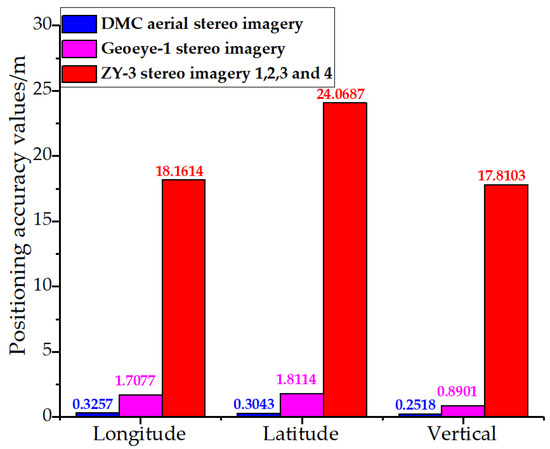
Figure 2.
The results of the assessment of the direct positioning accuracy for the multi-sensor multi-resolution imagery including the ZY-3, the Geoeye-1 satellite imagery, and the DMC aerial stereo imagery.
4.2. Results Comparison of Using Weighted Schemes, Unweighted Schemes, and Free Network Bundle Adjustment
According to the experimental design in Section 3.2.1, the comparative results of using weighted schemes, unweighted schemes, and free network bundle adjustment are summarized in Table 3. From Table 3, it is clear that, for all the imagery scenarios, the geometric positioning accuracy based on the network bundle adjustment exists the worst, no matter in planar direction, vertical direction, or overall directions. The geometric positioning accuracy experienced a dramatic increase when using weighted schemes and unweighted schemes. Specifically, the case using unweighted schemes achieved the second-best positioning accuracy in planimetry, height, and overall directions. When using the weighted schemes, the geometric positioning accuracy in overall directions experience an increase compared with the case of using the unweighted schemes, that is, the case of using the weighted schemes achieved the best geometric positioning accuracy. Taking the imagery scenario d for example, the results of using the unweighted schemes were 4.516 m in planar direction, 2.085 m in vertical direction, and 4.974 m in overall directions, while the geometric positioning accuracy of using the weighted schemes were 3.913 m, 2.161 m, and 4.470 m in planar, vertical, and overall directions, respectively. Therefore, the following performance tests were all based on the weighted schemes.
Table 3.
The comparative results of using weighted schemes, unweighted schemes, and free network bundle adjustment.
4.3. Overall Accuracy Evaluation of Using One Stereo Imagery as Reference Imagery
As described in Section 3.2.2, the Geoeye-1 and ZY-3 satellite stereoscopic imagery are selected for the assessment. A number of concentric circles with a radius of (n = 1, 2, 3, ……) and the circle center of the smallest circumscribed circle for the reference image area were constructed. Subsequently, the RMSEs of the GPS checkpoints within each circumscribed circle were calculated as the geometric positioning accuracy of the area within this concentric circle for assessment and comparison.
Table 4 gives the overall geometric positioning accuracies of the area within each concentric circle for the five different image combination scenarios, which all used the Geoeye-1 stereo imagery as the reference imagery, and the corresponding overall accuracies are illustrated in Figure 3. From Table 4, it can be seen that there are differences in the geometric positioning accuracy for the bundle adjustments using the five different image combination scenarios. As shown in Figure 3, for all ranges, the combination scenario using Geoeye-1 stereo imagery and ZY-3 stereo imagery 1 and 3 achieved the best overall geometric positioning accuracy of 4.172 m, which is basically equal to the results of the combination scenarios a and c (4.524 m and 4.470 m overall accuracy, respectively). With the increase of the statistical area covered by the lower-resolution stereo imagery, the results of bundle adjustments using the same Geoeye-1 stereo imagery as the reference imagery were decreased. The combination scenario using the Geoeye-1 stereo imagery and the ZY-3 stereo imagery 1, 2, 3, and 4 obtained the worst results, with an overall accuracy of 7.250 m. For each individual combination scheme, as shown in Figure 3, the overall geometric positioning error values show an upward trend with increasing statistical area, which means that the credibility of the determined ground points gradually decreases with increasing statistical area. This shows that the accuracy of the bundle adjustments can no longer meet the requirements for high-precision mapping applications when the lower-resolution image area increases to a certain level. Therefore, it is necessary to further quantitatively assess the geometric positioning performance of reference images for the accuracy enhancement of lower-resolution images.
Table 4.
The overall geometric positioning accuracy of the area within the concentric circle with a radius of (n = 1, 2, 3, ……) and the circle center of the smallest circumscribed circle for the reference image area.
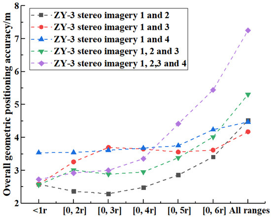
Figure 3.
Illustration of the overall geometric positioning accuracy within the concentric circle with a radius of (n = 1, 2, 3, ……) and the circle center of the smallest circumscribed circle for the reference image area in 5 different image combination scenarios.
For further assessment, the RMSEs of the GPS checkpoints within the radius circumscribed circle and outside the (n = 1, 2, 3, ……) radius circumscribed circle are calculated as the geometric positioning accuracy of the area within radius circumscribed circle and outside (n = 1, 2, 3, ……) radius circumscribed circle for further evaluation and experimental analysis. As described in [39,40,41], the imagery data (which should be at least three times more accurate than the evaluated data) are used for evaluating the accuracy of the evaluated data. In Section 4.1, the Geoeye-1 stereo imagery achieved a considerable direct geometric positioning accuracy of 1.811 m, 1.708 m, 0.890 m, and 2.644 m in longitude, latitude, elevation, and overall directions, respectively. Therefore, in this case study, an accuracy of 7 m, which is more than three times more inaccurate than the Geoeye-1 stereo imagery, is used as the criterion for the evaluation: that is, the determined points in the area where the geometric positioning accuracy is greater than 7 m are considered to be untrustworthy.
The results of the overall absolute positioning accuracy of the area within the concentric circle with a radius of (n = 1, 2, 3, ……) and outside the (n = 1, 2, 3, ……) radius circumscribed circle in the five different image combination scenarios are summarized in Table 5, and the corresponding overall accuracies are illustrated in Figure 4. From the figure, it is clear that the five combination scenarios exhibit basically the same overall geometric positioning accuracy within the circular area with a radius of 4 ∗ r. The overall results fluctuate between 2.038 and 4.825 m, which are all far less than 7 m. When the area increases to an area with a radius of 5 ∗ r, the combination scenario using the Geoeye-1 stereo imagery and the ZY-3 stereo imagery 1, 2, 3, and 4 achieved the worst overall geometric positioning accuracy of 7.609 m. The determined points for the area with a radius of 4 ∗ r–5 ∗ r are considered to be untrustworthy. The remaining combination scenarios also achieved an overall positioning accuracy of less than 7 m. As the area of the circle continues to increase, an increasing number of combination scenarios achieved an overall geometric positioning accuracy greater than 7 m. When the radius of the area is greater than 6 ∗ r, the results were pretty disastrous.
Table 5.
The overall geometric positioning accuracy of the area within the concentric circle with a radius of (n = 1, 2, 3, ……) and outside the (n = 1, 2, 3, ……) radius circumscribed circle in the five different image combination scenarios.

Figure 4.
Illustration of the overall geometric positioning accuracy within the concentric circle with a radius of (n = 1, 2, 3, ……) and outside the (n = 1, 2, 3, ……) radius circumscribed circle for the five different image combination scenarios.
Therefore, in this case study, the area with the circular center of the smallest circumscribed circle of the Geoeye-1 stereo reference image area and a radius of 4 ∗ r is regarded as an effective area. If the low-resolution image area continues to increase, it is best to add other reference images outside the area greater than 4 ∗ r radius to achieve high-precision geometric positioning for the whole image area.
4.4. Geometric Positioning Using Aerial Imagery as Reference Imagery
To verify the adaptability of the method presented in this paper to the DMC aerial imagery, six imagery combination scenarios are adopted for analysis. The imagery combination scenarios and the corresponding accuracy results are summarized in Table 6, including accuracies for all ranges and accuracies outside the overlapping area. Figure 5 shows the planimetric and height accuracy level curves of the geometric integration using aerial imagery as reference imagery for the six imagery combination scenarios.
Table 6.
The geometric integration results using aerial imagery as reference imagery for the reference-imagery-based bundle adjustments in six image combination scenarios.
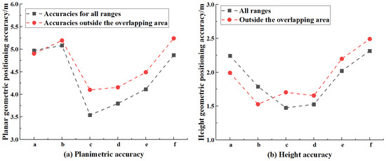
Figure 5.
Illustration of the geometric positioning accuracy including planimetric accuracy and height accuracy by integrating the aerial imagery and the lower-resolution ZY-3 satellite imagery for the reference-imagery-based bundle adjustments. a, b, c, d, e, and f represent the six different imagery combination scenarios. a. Single aerial imagery 119057 + ZY-3 stereo imagery 1; b. single aerial imagery 119058 + ZY-3 stereo imagery 1; c. stereo aerial imagery + ZY-3 stereo imagery 1; d. stereo aerial imagery + ZY-3 stereo imagery 1 and 2; e. stereo aerial imagery + ZY-3 stereo imagery 1, 2, and 3; f. stereo aerial imagery + ZY-3 stereo imagery 1, 2, 3, and 4.
From Figure 5, it can be seen that the combined geometric positioning using aerial imagery as reference imagery for bundle adjustments is able to improve the geometric positioning accuracy for the entire lower-resolution imagery and shows a similar pattern. Specifically, for the combination scenarios using a single aerial imagery as the reference imagery, the geometric positioning values for all ranges and outside the overlapping region are generally similar, with values of around 5.0 m in the horizontal direction and fluctuating between values of 1.52 and 2.24 m in the vertical direction. When one pair of aerial stereo images are used as the reference images, the horizontal accuracy increases dramatically, reaching 3.543 m for all regions and 4.100 m outside the overlapping area. Additionally, the height accuracy experiences a slight increase from 1.789 to approximately 1.475 m for all ranges, while the accuracy value outside the overlapping area suffers a slight decline. Afterwards, with the increase of the area covered by the lower-resolution ZY-3 stereo imagery, the planimetric and height accuracy exhibit almost the same downward tendency for all ranges and the range outside the overlapping area. For the imagery combination scenario using one stereo aerial imagery and two ZY-3 stereo imagery, there is a slight decline in accuracy for both all ranges and the area outside the overlapping area. Specifically, in the case of all ranges, the accuracy values experience a gentle decrease from less than 3.5 m to approximately 3.79 m in the planar direction and from 1.47 m to around 1.52 m in elevation compared with the combination scenario using one stereo aerial imagery and one ZY-3 stereo imagery. Furthermore, the accuracy outside the overlapping area displays a lesser downward tendency in the planimetric and height directions. It is noteworthy that all the accuracies suffer a dramatic decline when increasing the range covered by the lower-resolution stereo imagery. As shown in Table 6 and Figure 5, the combination scenario using one stereo aerial imagery and four ZY-3 stereo imageries achieved the worst results for all ranges, with values stable at around 4.8 m in planimetry and 2.3 m in elevation. The area outside the overlapping area exhibited worse geometric positioning accuracy, with values of about 5.24 m in the planimetric direction and 2.492 m in the height direction.
4.5. Combined Geometric Positioning Using Multi-Stereo Heterogeneous Imagery as Reference Imagery Based on Adaptive Weights
4.5.1. Performance Analysis for All Ranges
The results of the combined geometric positioning using multi-sensor multi-stereo heterogeneous imagery as the references are summarized in Table 7, and Figure 6 shows the overall geometric positioning level curves of the combined geometric positioning tests using the method.
Table 7.
The overall geometric integration results when using multi-sensor multi-stereo heterogeneous imagery as the reference imagery for the reference-imagery-based bundle adjustments for four image combination scenarios.
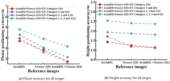
Figure 6.
The geometric positioning level curves in planimetry and height of the geometric integration tests using the presented reference-imagery-based bundle adjustments with three stereo reference imagery selections tested. Note: S—stereo.
From Table 7 and Figure 6, it is clear that the overall geometric positioning accuracy is high in the four imagery combination scenarios when using multi-sensor multi-stereo heterogeneous imagery as the reference imagery. However, there are still many big differences for different imagery combination scenarios and different stereo reference imagery selections. Specifically, the case using stereo aerial imagery as references achieved the worst positioning accuracy in planimetry and height, while it achieved the second-best planar and height accuracy when using the stereo Geoeye-1 imagery as reference imagery. When combining the stereo DMC aerial imagery and the stereo Geoeye-1 imagery as references, the planar accuracy for all ranges experiences a slight increase compared with the case of using the stereo Geoeye-1 imagery and suffers an apparent decline compared with the results generated from the stereo aerial reference-imagery-based bundle adjustments. However, even though the height accuracy values display a dramatic decrease compared with the case that uses the stereo DMC aerial imagery as references, they exhibit a slight decrease compared with the results based on the stereo Geoeye-1 imagery. One of the possible explanations for this difference in this case study is that the stereo aerial imagery achieves almost the same geometric positioning accuracy in height as the stereo Geoeye-1 imagery, so using a combination of these two heterogeneous stereo images as references can achieve a higher accuracy in the height direction. Nonetheless, the stereo aerial imagery has a far worse performance in planimetry than the stereo Geoeye-1 imagery due to the much smaller image format. The accuracy in the horizontal direction using the DMC aerial imagery and the stereo Geoeye-1 imagery as references is susceptible to the stereo Geoeye-1 imagery with a larger image format. Consequently, in such cases, the planar accuracy shows a slight decrease while the height accuracy exhibits a moderate enhancement compared with the case of using the stereo Geoeye-1 imagery as references.
The geometric positioning level curves in planimetry and the height of the geometric integration tests using the presented method with four imagery combination scenarios tested are shown in Figure 7. From the figure, it can be seen that the horizontal and height accuracy values exhibit an upward trend with the increase of the coverage area of the ZY-3 stereo imagery for three reference imagery selections; this is in agreement with the results of the processing of the stereo Geoeye-1 imagery and the stereo DMC aerial imagery in the previous section.
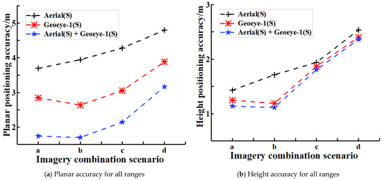
Figure 7.
The geometric positioning level curves in planimetry and height of the geometric integration tests using the presented reference-imagery-based bundle adjustments with four imagery combination scenarios tested. a. Aerial (S) + Geoeye-1 (S) + ZY-3 imagery 1 (S); b. Aerial (S) + Geoeye-1 (S) + ZY-3 imagery 1 and 2 (S); c. Aerial (S) + Geoeye-1 (S) + ZY-3 imagery 1, 2, and 3 (S); and d. Aerial (S) + Geoeye-1 (S) + ZY-3 imagery 1, 2, 3, and 4 (S). Note: S—stereo.
4.5.2. Performance Analysis outside the Overlapping Area
To evaluate the performance of the positioning accuracy outside the overlapping area using multi-stereo heterogeneous imagery as reference imagery, the geometric positioning level curves outside the overlapping area with three different reference imagery selections in four imagery combination scenarios are provided in Figure 8.
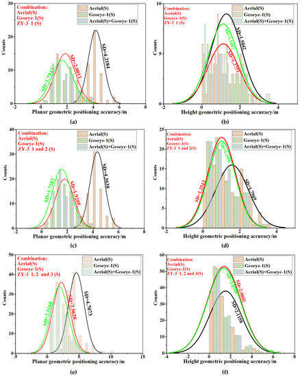
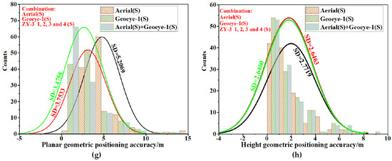
Figure 8.
The geometric positioning level curves outside the overlapping area with three different reference imagery selections in four imagery combination scenarios. (a,b) Aerial (S) + Geoeye-1 (S) + ZY-3 imagery 1 (S); (c,d) Aerial (S) + Geoeye-1 (S) + ZY-3 imagery 1 and 2 (S); (e,f) Aerial (S) + Geoeye-1 (S) + ZY-3 imagery 1, 2, and 3 (S); (g,h) Aerial (S) + Geoeye-1 (S) + ZY-3 imagery 1, 2, 3, and 4 (S). Note: SD–Standard Deviation; S—stereo.
The results in Figure 8 show that the positioning accuracy for the ZY-3 stereo imagery outside the overlapping area can be improved for three different reference imagery selections, even if the reference image only covers a small portion of the ZY-3 stereo imagery. However, it is different in the positioning enhancement, which uses different heterogeneous stereo imagery to improve the geometric positioning accuracy of the ZY-3 stereo imagery outside the overlapping area. For instance, as shown in the first imagery combination scenario in Figure 8, the DMC aerial stereo imagery can achieve a planar accuracy and height accuracy of 4.218 m and 1.504 m, respectively; meanwhile, for the Geoeye-1 stereo imagery, the corresponding values are 2.001 and 1.375 m, respectively, which are all better than the results for the DMC aerial stereo imagery. From Figure 8 and Table 7, it can be seen that the positioning accuracy for the ZY-3 stereo imagery outside the overlapping area is generally similar to the overall geometric positioning accuracy. It is interesting that, in this case study, the DMC stereo imagery achieved a moderately worse planar and height accuracy than the accuracies for all ranges in the four imagery combination scenarios, and achieved a slightly better accuracy in the horizontal direction in the first three imagery combination scenarios and slightly worse accuracy in the horizontal direction in the fourth imagery combination scenario for the Geoeye-1 stereo imagery. When combining the stereo DMC aerial imagery and the stereo Geoeye-1 imagery as references, the planar accuracy values for the area outside the overlapping area experienced a moderate increase compared with the case of using the stereo Geoeye-1 imagery, and suffered a decline compared with the results generated from the stereo aerial reference-imagery-based bundle adjustments. For example, for the last imagery combination scenario, the accuracy values increase from 3.753 to 3.476 m and 2.772 to 2.646 m in the horizontal and height directions, respectively, compared with the case of using the stereo Geoeye-1 imagery.
Additionally, Figure 9 also gives the geometric positioning level curves outside the overlapping area using the presented bundle adjustments with the four tested imagery combination scenarios. From the figure, it can be seen that the horizontal and height accuracy values outside the overlapping area have a similar tendency with the increase of the coverage area of the ZY-3 stereo imagery for the three reference imagery selections. Thus, if the area of the ZY-3 stereo imagery continues to increase, the impact of the increasing area on the geometric positioning accuracy for all ranges and the area outside the overlapping area can be improved by adding more stereo imagery with an equal or higher positioning accuracy.
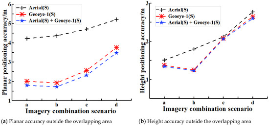
Figure 9.
The geometric positioning level curves for the area outside the overlapping area using the presented bundle adjustments with the four tested imagery combination scenarios. a. Aerial (S) + Geoeye-1 (S) + ZY-3 imagery 1 (S); b Aerial (S) + Geoeye-1 (S) + ZY-3 imagery 1 and 2 (S); c. Aerial (S) + Geoeye-1 (S) + ZY-3 imagery 1, 2, and 3 (S); and d. Aerial (S) + Geoeye-1 (S) + ZY-3 imagery 1, 2, 3, and 4 (S). Note: S—stereo.
5. Conclusions
Combined geometric positioning using images with different resolutions and imaging sensors is being increasingly widely utilized in practical engineering applications. In this work, we attempt to perform the combined geometric positioning and performance analysis of multi-resolution optical images from satellite and aerial platforms based on weighted RFM bundle adjustment. We conduct experiments using a case study in Shanghai with ZY-3 satellite imagery, GeoEye-1 satellite imagery, and DMC aerial imagery to validate the following questions, including the effectiveness of the proposed weighted method, quantitative evaluation of the constrained performance of using one stereo image as a reference for positioning, the adaptability of the weighted method to aerial imagery (single and stereo imagery) and some special cases (for example, there is only one high-precision image), and the combined positioning of multi-stereo heterogeneous images based on the weighted method. In future work, we would explore the effect of the distribution of high-accuracy images on the combined positioning by using this weighted method. The following are some conclusions drawn from the experimental results.
(1) The alternative model of the combined geometric positioning of multi-sensor multi-resolution optical images from satellite and aerial platforms based on weighted RFM bundle adjustment can obtain better positioning accuracy compared with the unweighted schemes. It can not only determine the weights adaptively, but is also suitable for some special cases, for example, there is only one high-precision image, that is, the method is able to improve the geometric positioning accuracy without GCPs for the multiple heterogeneous images with lower positioning accuracy by using a single reference image, a pair of stereo reference images, or multiple pairs of stereo reference images.
(2) The effective area of using one stereo image as a reference for positioning is limited, and the constrained performance is quantitatively evaluated. In the case study in Shanghai, the area with the circular center of the smallest circumscribed circle of the Geoeye-1 stereo reference image area and a radius of 4 ∗ r is regarded as an effective area that the Geoeye-1 stereo reference image can work. If the low-resolution image area continues to increase, it is best to add other reference images outside the area of greater than 4 ∗ r radius to achieve high-precision geometric positioning for the whole image area.
(3) The adaptability of the method to aerial imagery is verified for the geometric combined positioning using single and stereo aerial imagery as reference imagery. In the case study, the case using a pair of stereo imagery as reference imagery displays a stronger capability to improve the overall positioning accuracy than the case using single imagery in both the planar and vertical directions. Additionally, all the accuracies for all ranges and the area outside the overlapping area suffer a dramatic decline when increasing the range covered by the lower-resolution stereo imagery.
(4) Multi-stereo heterogeneous imagery such as aerial stereo imagery and push-broom scanning imagery can be combined as reference imagery to further improve the geometric positioning accuracy for all ranges and the area outside the overlapping area.
Author Contributions
Conceptualization, W.S. and S.L.; methodology, W.S., S.L. and C.N.; validation, W.S., S.L. and C.N.; formal analysis, W.S. and S.L.; writing—original draft preparation, W.S. and S.L.; writing—review and editing, S.L., X.T., Y.J. and Z.Y.; Funding acquisition, S.L.,Y.J. and X.T. All authors have read and agreed to the published version of the manuscript.
Funding
This work was supported in part by the National Key R&D Program of China (Project No. 2017YFB0502903), National Natural Science Foundation of China (Project No. 41771483, 41631178 and 41601414), funds from the State Key Laboratory of Geo-Information Engineering (Project No. SKLGIE2018-Z-3-2), research fund of the State Key Laboratory for Disaster Reduction in Civil Engineering (Project No. SLDRCE19-B-36), and Fundamental Research Funds for the Central Universities.
Data Availability Statement
Data available on request due to restrictions eg privacy or ethical. The data presented in this study are available on request from the corresponding author.
Conflicts of Interest
The authors declare no conflict of interest.
References
- Honkavaara, E.; Arbiol, R.; Markelin, L.; Martinez, L.; Cramer, M.; Bovet, S.; Schläpfer, D. Digital airborne photogrammetry—A new tool for quantitative remote sensing—A state-of-the-art review on radiometric aspects of digital photogrammetric images. Remote Sens. 2009, 1, 577. [Google Scholar] [CrossRef]
- Manfreda, S.; McCabe, M.F.; Miller, P.E.; Lucas, R.; Pajuelo, M.V.; Mallinis, G.; Ben Dor, E.; Helman, E.; Estes, D.L.; Ciraolo, G.; et al. On the use of unmanned aerial systems for environmental monitoring. Remote Sens. 2018, 10, 641. [Google Scholar] [CrossRef]
- Yao, H.; Qin, R.J.; Chen, X.Y. Unmanned aerial vehicle for remote sensing applications—A review. Remote Sens. 2019, 11, 1443. [Google Scholar] [CrossRef]
- Song, H.; Srinivasan, R.; Sookoor, T.; Jeschke, S. Smart Cities: Foundations, Principles and Applications; Wiley: Hoboken, NJ, USA, 2017; pp. 1–20. [Google Scholar]
- Song, H.; Rawat, D.; Jeschke, S.; Brecher, C. Cyber-Physical Systems: Foundations, Principles and Applications; Academic Press: Boston, MA, USA, 2016; pp. 20–30. [Google Scholar]
- Di, K.C.; Ma, R.J.; Li, R.X. Geometric processing of Ikonos stereo imagery for coastal mapping applications. Photogramm. Eng. Remote Sens. 2003, 69, 873–879. [Google Scholar]
- Xu, L.; Jing, W.; Song, H.; Chen, G. High-Resolution Remote Sensing Image Change Detection Combined with Pixel-Level and Object-Level. IEEE Access 2019, 7, 78909–78918. [Google Scholar] [CrossRef]
- Yang, X.J.; Li, J. Advances in Mapping from Remote Sensor Imagery: Techniques and Applications; CRC Press: Boca Raton, FL, USA, 2012. [Google Scholar]
- Zanutta, A.; Lambertini, A.; Vittuari, L. UAV photogrammetry and ground surveys as a mapping tool for quickly monitoring shoreline and beach changes. J. Mar. Sci. Eng. 2018, 8, 52. [Google Scholar] [CrossRef]
- Ji, J.; Jing, W.; Chen, G.; Lin, J.; Song, H. Multi-Label Remote Sensing Image Classification with Latent Semantic Dependencies. Remote Sens. 2020, 12, 1110. [Google Scholar] [CrossRef]
- Ferrari, A.; Dazzi, S.; Vacondio, R.; Mignosa, P. Enhancing the resilience to flooding induced by levee breaches in lowland areas: A methodology based on numerical modelling. Nat. Hazards Earth Syst. Sci. 2020, 20, 59–72. [Google Scholar] [CrossRef]
- Santos, D.; Alex, J.; Gosselin, P.H.; Philipp-Foliguet, S.; Torres, R.D.S.; Falcao, A.X. Interactive multiscale classification of high-resolution remote sensing images. IEEE J. Sel. Top. Appl. Earth Obs. Remote Sens. 2013, 6, 2020–2034. [Google Scholar] [CrossRef]
- Fan, H.; Su, H.; Guibas, L.J. A Point Set Generation Network for 3D Object Reconstruction from a Single Image. In Proceedings of the IEEE Conference on Computer Vision and Pattern Recognition, Honolulu, HI, USA, 21–26 July 2017; pp. 605–613. [Google Scholar]
- Li, D.R.; Zhang, G.; Jiang, W.S.; Yuan, X.X. SPOT-5 HRS Satellite Imagery Block Adjustment without GCPS or with Single GCP. Geomat. Inf. Sci. Wuhan Univ. 2006, 31, 377–381. [Google Scholar]
- Lv, Z.; Song, H.; Basanta-Val, P.; Steed, A.; Jo, M. Next-Generation Big Data Analytics: State of the Art, Challenges, and Future Research Topics. IEEE Trans. Ind. Inform. 2017, 13, 1891–1899. [Google Scholar] [CrossRef]
- Jiang, B.; Yang, J.; Xu, H.; Song, H.; Zheng, G. Multimedia Data Throughput Maximization in Internet-of-Things System Based on Optimization of Cache-Enabled UAV. IEEE Internet Things J. 2019, 6, 3525–3532. [Google Scholar] [CrossRef]
- Hu, Y.; Tao, V.; Croitoru, A. Understanding the rational function model: Methods and applications. Int. Arch. Photogramm. Remote Sens. 2004, 20, 119–124. [Google Scholar]
- Liu, J.; Zhang, Y.S.; Wang, D.H. Precise Positioning of High Spatial Resolution Satellite Images Based on RPC Models. Acta Geod. Cartogr. Sin. 2006, 35, 30–34. [Google Scholar]
- Li, D.R. China’s first civilian three-line-array stereo mapping satellite: ZY-3. Acta Geod. Cartogr. Sin. 2012, 41, 317–322. [Google Scholar]
- Liu, Y.; Weng, X.; Wan, J.; Yue, X.; Song, H.; Vasilakos, A.V. Exploring Data Validity in Transportation Systems for Smart Cities. IEEE Commun. Mag. 2017, 55, 26–33. [Google Scholar] [CrossRef]
- Sheng, Y. Theoretical analysis of the iterative photogrammetric method to determining ground coordinates from photo coordinates and a DEM. Photogramm. Eng. Remote Sens. 2005, 71, 863–871. [Google Scholar] [CrossRef]
- Teo, T.A.; Chen, L.C.; Liu, C.L.; Tung, Y.C.; Wu, W.Y. DEM-aided block adjustment for satellite images with weak convergence geometry. IEEE Trans. Geosci. Remote Sens. 2009, 48, 1907–1918. [Google Scholar]
- Zhang, Y.J.; Wan, Y.; Huang, X.; Ling, X. DEM-assisted RFM block adjustment of pushbroom nadir viewing HRS imagery. IEEE Trans. Geosci. Remote Sens. 2015, 54, 1025–1034. [Google Scholar] [CrossRef]
- Ling, X.; Zhang, Y.J.; Xiong, J.; Huang, X.; Chen, Z. An image matching algorithm integrating global SRTM and image segmentation for multi-source satellite imagery. Remote Sens. 2016, 8, 672. [Google Scholar] [CrossRef]
- Zheng, M.T.; Zhang, Y.J. DEM-aided bundle adjustment with multisource satellite imagery: ZY-3 and GF-1 in large areas. IEEE Geosci. Remote Sens. Lett. 2016, 13, 880–884. [Google Scholar] [CrossRef]
- Zhang, H.; Zhang, G.; Jiang, Y.H.; Wang, T. A SRTM-DEM-controlled ortho-rectification method for optical satellite remote sensing stereo images. Acta Geod. Cartogr. Sin. 2016, 45, 326–336. [Google Scholar]
- Wang, M.; Yang, B.; Pan, J.; Jin, S. High Precision Geometric Processing and Application of High Resolution Optical Satellite Remote Sensing Image; Science Press: Beijing, China, 2017. [Google Scholar]
- Zhou, P.; Tang, X.M.; Wang, Z.; Cao, N.; Wang, X. SRTM-assisted block adjustment for stereo pushbroom imagery. Photogramm. Rec. 2018, 33, 49–65. [Google Scholar] [CrossRef]
- Wu, B.; Guo, J.; Zhang, Y.; King, B.A.; Chen, Y. Integration of Chang’E-1 imagery and laser altimeter data for precision lunar topographic modeling. IEEE Trans. Geosci. Remote Sens. 2011, 49, 4889–4903. [Google Scholar]
- Wu, B.; Hu, H.; Guo, J. Integration of Chang’E-2 imagery and LRO laser altimeter data with a combined block adjustment for precision lunar topographic modeling. Earth Planet. Sci. Lett. 2014, 6, 1–15. [Google Scholar] [CrossRef]
- Li, G.Y.; Tang, X.M.; Gao, X.; Wang, H.; Wang, Y. ZY-3 Block adjustment supported by glas laser altimetry data. Photogramm. Rec. 2016, 31, 88–107. [Google Scholar] [CrossRef]
- Li, G.Y.; Tang, X.M.; Gao, X.; Wang, X.; Fan, W.; Chen, J.; Mo, F. Integration of ZY3-02 Satellite Laser Altimetry Data and Stereo Images for High-Accuracy Mapping. Photogramm. Eng. Remote Sens. 2018, 84, 569–578. [Google Scholar] [CrossRef]
- Zhang, G.; Xu, K.; Jia, P.; Hao, X.; Li, D.R. Integrating Stereo Images and Laser Altimeter Data of the ZY3-02 Satellite for Improved Earth Topographic Modeling. Remote Sens. 2019, 11, 2453. [Google Scholar] [CrossRef]
- Guérin, C. Effect of the DTM quality on the bundle block adjustment and orthorectification process without GCP: Exemple on a steep area. In Proceedings of the 2017 IEEE International Geoscience and Remote Sensing Symposium (IGARSS), Fort Worth, TX, USA, 23–28 July 2017; pp. 1067–1070. [Google Scholar]
- Ali-Sisto, D.; Gopalakrishnan, R.; Kukkonen, M.; Savolainen, P.; Packalen, P. A method for vertical adjustment of digital aerial photogrammetry data by using a high-quality digital terrain model. Int. J. Appl. Earth Obs. Geoinf. 2020, 84, 954–1963. [Google Scholar] [CrossRef]
- Niu, X.; Zhou, F.; Di, K.C.; Li, R.X. 3D geopositioning accuracy analysis based on integration of QuickBird and IKONOS imagery. In Proceedings of the ISPRS Hannover Workshop 2005 in High Resolution Earth Imaging for Geospatial Information, Hannover, Germany, 17–20 May 2005. [Google Scholar]
- Eisenbeiss, H.; Baltsavias, E.; Pateraki, M.; Zhang, L. Potential of IKONOS and QUICKBIRD imagery for accurate 3D-Point positioning, orthoimage and DSM generation. Int. Arch. Photogramm. Remote Sens. Spat. Inf. Sci. 2004, 5, 522–528. [Google Scholar]
- Li, R.X.; Zhou, F.; Niu, X.T.; Di, K.C. Integration of Ikonos and QuickBird imagery for geopositioning accuracy analysis. Photogramm. Eng. Remote Sens. 2007, 73, 1067–1076. [Google Scholar]
- Li, R.X.; Deshpande, S.; Niu, X.T.; Zhou, F.; Di, K.C.; Wu, B. Geometric integration of aerial and high-resolution satellite imagery and application in shoreline mapping. Mar. Geod. 2008, 31, 143–159. [Google Scholar] [CrossRef]
- Jaehoon, J.; Kim, T. 3-D geopositioning by combination of images from different sensors based on a rigorous sensor model. J. Korean Soc. Surv. Geod. Photogramm. Cartogr. 2009, 31, 11–19. [Google Scholar]
- Tong, X.H.; Liu, S.J.; Xie, H.; Wang, W.; Chen, P.; Bao, F. Geometric integration of aerial and QuickBird imagery for high accuracy geopositioning and mapping application: A case study in Shanghai. Mar. Geod. 2010, 33, 437–449. [Google Scholar] [CrossRef]
- Jaehoon, J. A study on the method for three-dimensional geo-positioning using heterogeneous satellite stereo images. J. Korean Soc. Surv. Geod. Photogramm. Cartogr. 2015, 33, 325–331. [Google Scholar] [CrossRef]
- Jeong, J.; Yang, C.; Kim, T. Geo-positioning accuracy using multiple-satellite images: IKONOS, QuickBird, and KOMPSAT-2 stereo images. Remote Sens. 2015, 7, 4549–4564. [Google Scholar] [CrossRef]
- Pan, X.C.; Jiang, T.; Yu, A.; Wang, X.; Zhang, Y. Geo-positioning of remote sensing images with reference image. J. Remote Sens. 2019, 23, 673–684. [Google Scholar]
- Tang, S.J.; Wu, B.; Zhu, Q. Combined adjustment of multi-resolution satellite imagery for improved geo-positioning accuracy. ISPRS J. Photogramm. Remote Sens. 2016, 114, 125–136. [Google Scholar] [CrossRef]
- Wang, J.; Liu, Y.X.; Yue, X.J.; Song, H.B.; Yuan, J.; Yang, T.; Seker, R. Integrating ground surveillance with aerial surveillance for enhanced amateur drone detection. Disruptive Technol. Inf. Sci. 2018, 10652, 1–7. [Google Scholar]
- Wang, J.; Liu, Y.X.; Niu, S.T.; Song, H.B. Beamforming-Constrained Swarm UAS Networking Routing. IEEE Trans. Netw. Sci. Eng. 2020, 1–13. [Google Scholar] [CrossRef]
- Wang, J.; Liu, Y.X.; Niu, S.T.; Song, H.B. Lightweight blockchain assisted secure routing of swarm UAS networking. Comput. Commun. 2020, 165, 131–140. [Google Scholar] [CrossRef]
- Wang, Z.; Ou, J.K. Determining the ridge parameter in a ridge estimation using L-curve method. Geomat. Inf. Sci. Wuhan Univ. 2004, 29, 235–238. [Google Scholar]
- Lin, X.Y.; Yuan, X.X. A Method for Solving Rational Polynomial Coefficients Based on Ridge Estimation. Geomat. Inf. Sci. Wuhan Univ. 2008, 33, 1130–1133. [Google Scholar]
- Song, W.P.; Zhang, B.; Niu, C.L.; Guo, L.L. An Integrated Matching Correction Algorithm based on Least Squares and Phase Correlation. Remote Sens. Technol. Appl. 2019, 34, 1296–1304. [Google Scholar]
- Fraser, C.S.; Hanley, H.B. Bias compensation in rational functions for IKONOS satellite imagery. Photogramm. Eng. Remote Sens. 2003, 69, 53–57. [Google Scholar] [CrossRef]
- Tong, X.H.; Liu, S.J.; Weng, Q. Bias-corrected rational polynomial coefficients for high accuracy geo-positioning of QuickBird stereo imagery. ISPRS J. Photogramm. Remote Sens. 2010, 65, 218–226. [Google Scholar] [CrossRef]
- Tong, X.H.; Liu, S.J.; Weng, Q.H. Geometric processing of QuickBird stereo imageries for urban land use mapping: A case study in Shanghai, China. IEEE J. Sel. Top. Appl. Earth Obs. Remote Sens. 2009, 2, 61–66. [Google Scholar] [CrossRef]
- Fischler, M.; Bolles, R. Random Sample Consensus: A Paradigm for Model Fitting with Applications to Image Analysis and Automated Cartography. Commun. ACM 1981, 24, 381–395. [Google Scholar] [CrossRef]
- Lowe, D. Distinctive Image Features from Scale-Invariant Keypoints. Int. J. Comput. Vis. 2004, 60, 91–110. [Google Scholar] [CrossRef]
- Gesch, D.B.; Maune, D. Digital Elevation Model Technologies and Applications: The DEM Users Manual, 2nd ed.; The National Elevation Dataset; American Society for Photogrammetry and Remote Sensing: Bethesda, MD, USA, 2007; pp. 99–118. [Google Scholar]
- Grohmann, C.H. Evaluation of TanDEM-X DEMs on selected Brazilian sites: Comparison with SRTM, ASTER GDEM and ALOS AW3D30. Remote Sens. Environ. 2018, 212, 121–133. [Google Scholar] [CrossRef]
- Wessel, B.; Huber, M.; Wohlfart, C.; Marschalk, U.; Kosmann, D.; Roth, A. Accuracy assessment of the global TanDEM-X Digital Elevation Model with GPS data. ISPRS J. Photogramm. Remote Sens. 2018, 139, 171–182. [Google Scholar] [CrossRef]
- Zhang, J.Q.; Pan, L.; Wang, S.G. Photogrammetry; Wuhan University Press: Wuhan, China, 2009. [Google Scholar]
- Zhang, Y.; Wang, T.; Feng, F.; Yuan, P.; Wang, X. Self-calibration block adjustment for Mapping Satellite-1three linear CCD image. J. Remote Sens. 2015, 19, 219–227. [Google Scholar]
- Cao, S.; Yuan, X. Refinement of RPCs Based on Systematic Error Compensation for Virtual Grid. Geomat. Inf. Sci. Wuhan Univ. 2011, 36, 185–190. [Google Scholar]
- Gong, J.; Wang, M.; Yang, B. High-precision Geometric Processing theory and Method of High-resolution Optical Remote Sensing Satellite Imagery without GCP. Acta Geod. Cartogr. Sin. 2017, 46, 1255–1261. [Google Scholar]
- Fraser, C.; Hanley, H. Bias-compensated RPCs for sensor orientation of high-resolution satellite imagery. Photogramm. Eng. Remote Sens. 2005, 71, 909–915. [Google Scholar] [CrossRef]
- Fraser, C.S.; Yamakawa, T. Insights into the affine model for high-resolution satellite sensor orientation. ISPRS J. Photogramm. Remote Sens. 2004, 5, 275–288. [Google Scholar] [CrossRef]
- Deng, X.; Yin, L.; Peng, S.; Ding, M. An iterative algorithm for solving ill-conditioned linear least squares problems. Geod. Geodyn. 2014, 6, 453–459. [Google Scholar] [CrossRef]
- Cox, D.D. Rank-Deficient and Discrete Ill-Posed Problems: Numerical Aspects of Linear Inversion. J. Am. Stat. Assoc. 1999, 94, 1388–1398. [Google Scholar] [CrossRef]
- Hansen, P.C.; Jensen, T.K.; Rodriguez, G. An adaptive pruning algorithm for the discrete L-curve criterion. J. Comput. Appl. Math. 2007, 198, 483–492. [Google Scholar] [CrossRef]
- Wang, R.X.; Wang, X.Y.; Wang, J.R.; Zao, F.; Li, J.; Chen, G. The interior accuracy estimation in the photogrammetric calculation of the stereoscopic imagery of The Chang’e-1. Sci. Surv. Mapp. 2008, 33, 5–9. [Google Scholar]
- Liu, C.B.; Li, D.; Xue, N. Surveying Satellite Imagery RPC Block Adjustment without Ground Control Points. Hydrogr. Surv. Charting 2018, 38, 17–20. [Google Scholar]
- Jiang, Y.H.; Wang, J.Y.; Zhang, L.; Zhang, G.; Li, X.; Wu, J.Q. Geometric Processing and Accuracy Verification of Zhuhai-1 Hyperspectral Satellites. Remote Sens. 2019, 11, 996. [Google Scholar] [CrossRef]
- Dartmann, G.; Song, H.; Schmeink, A. Big Data Analytics for Cyber-Physical Systems: Machine Learning for the Internet of Things; Elsevier: Amsterdam, The Netherlands, 2019; pp. 1–20. [Google Scholar]
- Jiang, Y.H.; Zhang, G.; Tang, X.M.; Li, D.R.; Wang, T.Y.; Huang, W.C.; Li, L.T. Improvement and assessment of the geometric accuracy of Chinese high-resolution optical satellites. IEEE J. Sel. Top. Appl. Earth Observ. Remote Sens. 2015, 8, 4841–4852. [Google Scholar] [CrossRef]
- Aguilar, M.A.; Saldaña, M.M.; Aguilar, F.J. GeoEye-1 and WorldView-2 pan-sharpened imagery for object-based classification in urban environments. Int. J. Remote Sens. 2013, 34, 2583–2606. [Google Scholar] [CrossRef]
- Liu, S.J.; Tong, X.H.; Wang, F.X.; Sun, W.Z.; Guo, C.C.; Ye, Z.; Jin, Y.M.; Xie, H.; Chen, P. Attitude jitter detection based on remotely sensed images and dense ground controls: A case study for Chinese ZY-3 satellite. IEEE J. Sel. Top. Appl. Earth Obs. Remote Sens. 2016, 9, 5760–5766. [Google Scholar] [CrossRef]
- Tilton, J.C.; Lin, G.Q.; Tan, B. Measurement of the band-to-band registration of the SNPP VIIRS imaging system from on-orbit data. IEEE J. Sel. Top. Appl. Earth Obs. Remote Sens. 2016, 10, 1056–1067. [Google Scholar] [CrossRef] [PubMed]
- Tilton, J.C.; Wolfe, R.E.; Lin, G.Q.; Dellomo, J.J. On-Orbit Measurement of the Effective Focal Length and Band-to-Band Registration of Satellite-Borne Whiskbroom Imaging Sensors. IEEE J. Sel. Top. Appl. Earth Obs. Remote Sens. 2019, 12, 4622–4633. [Google Scholar] [CrossRef] [PubMed]
Publisher’s Note: MDPI stays neutral with regard to jurisdictional claims in published maps and institutional affiliations. |
© 2021 by the authors. Licensee MDPI, Basel, Switzerland. This article is an open access article distributed under the terms and conditions of the Creative Commons Attribution (CC BY) license (http://creativecommons.org/licenses/by/4.0/).