
Detecting the Turning Points of Grassland Autumn Phenology on the Qinghai-Tibetan Plateau: Spatial Heterogeneity and Controls

 , and
, and 
Abstract
: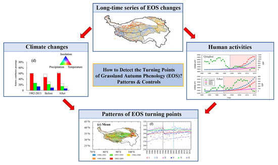
1. Introduction
2. Materials and Methods
2.1. Study Area
2.2. Data Source
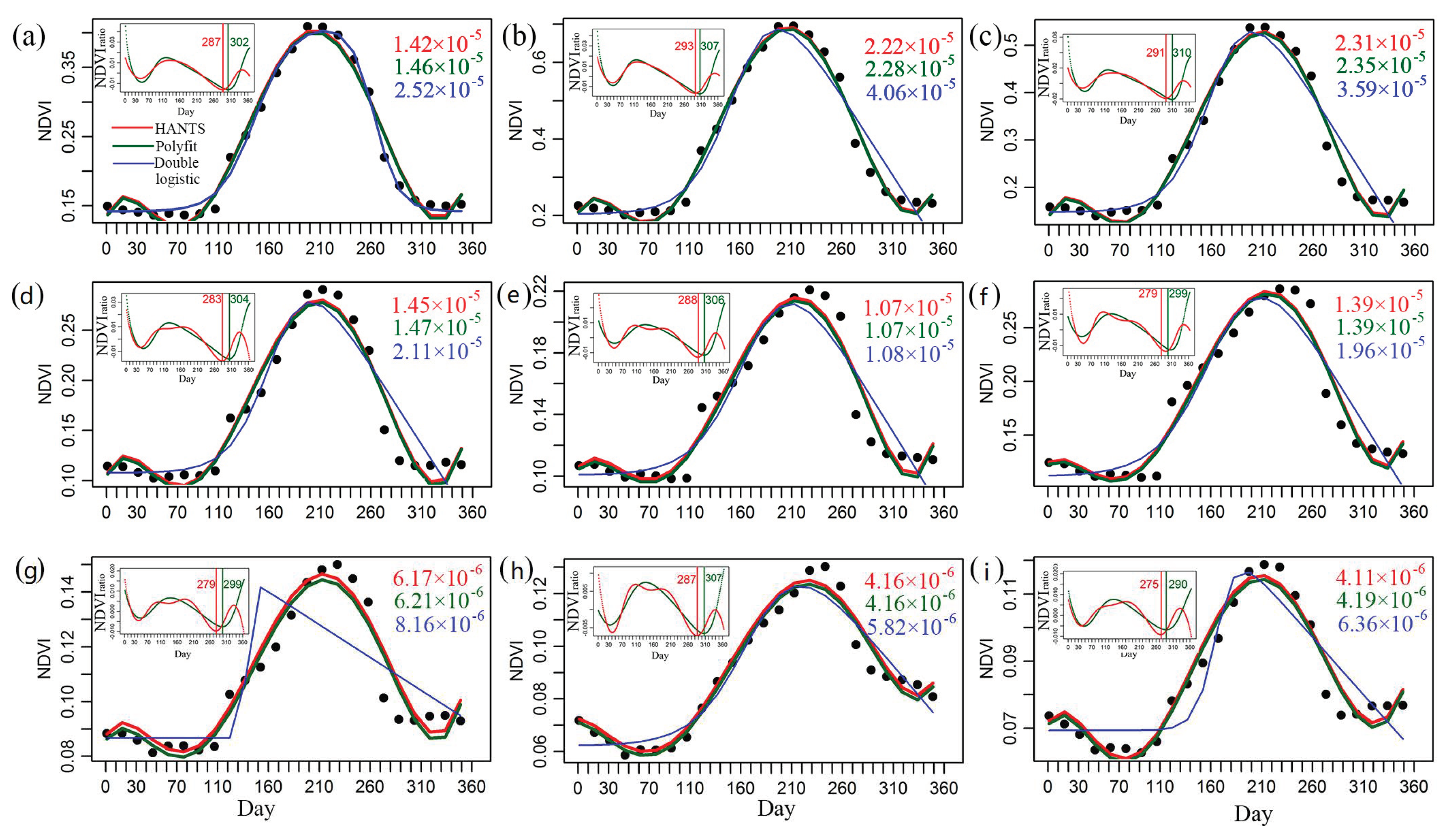
2.3. Retrieval of EOS
2.4. Quantification of the EOS Trends, Turning Points, and Controls
3. Results
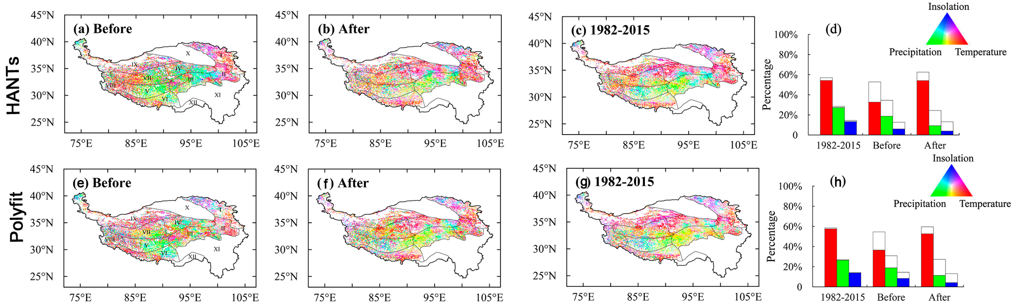
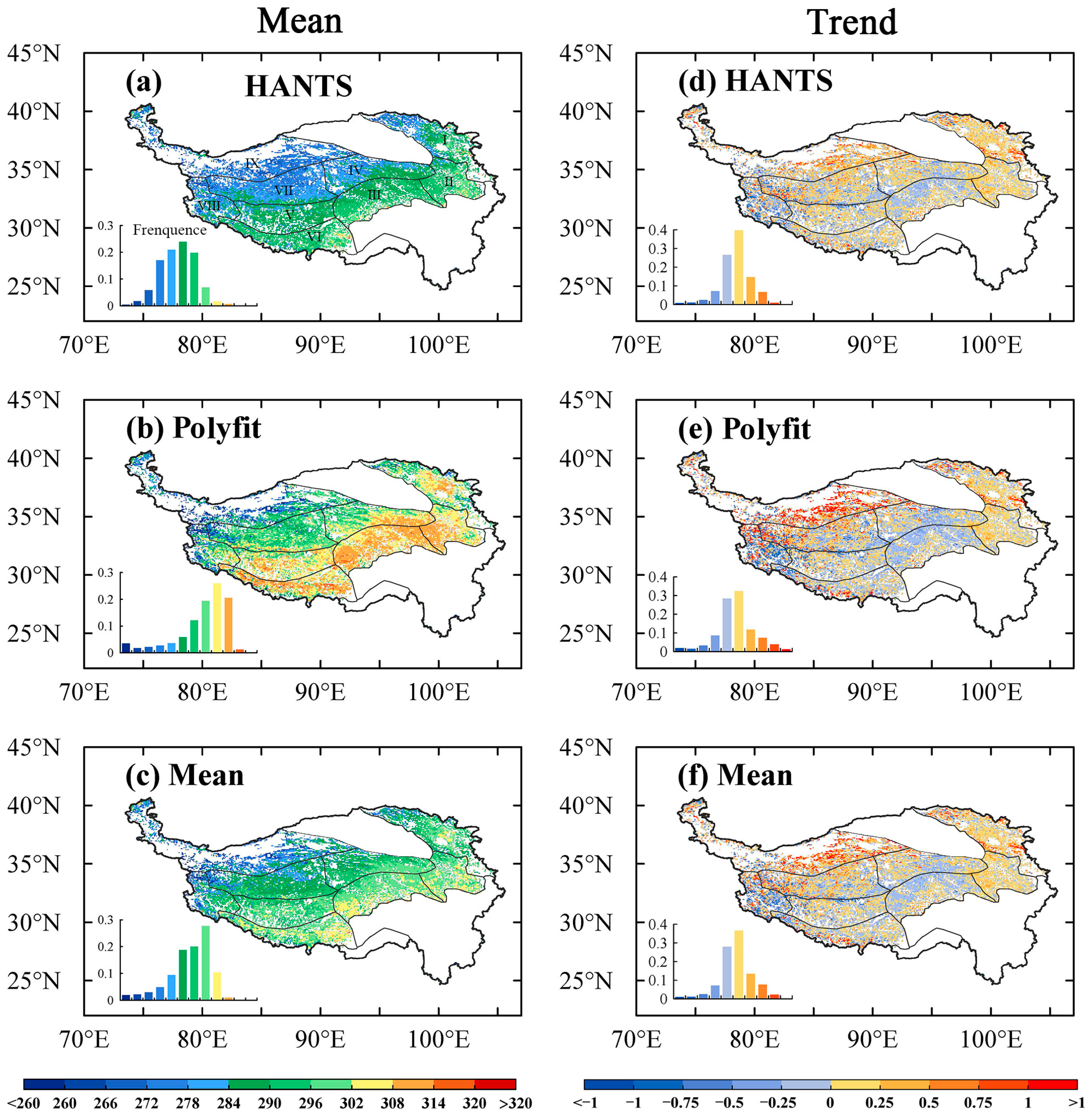
3.1. EOS Spatial Distribution and Variation Characteristics
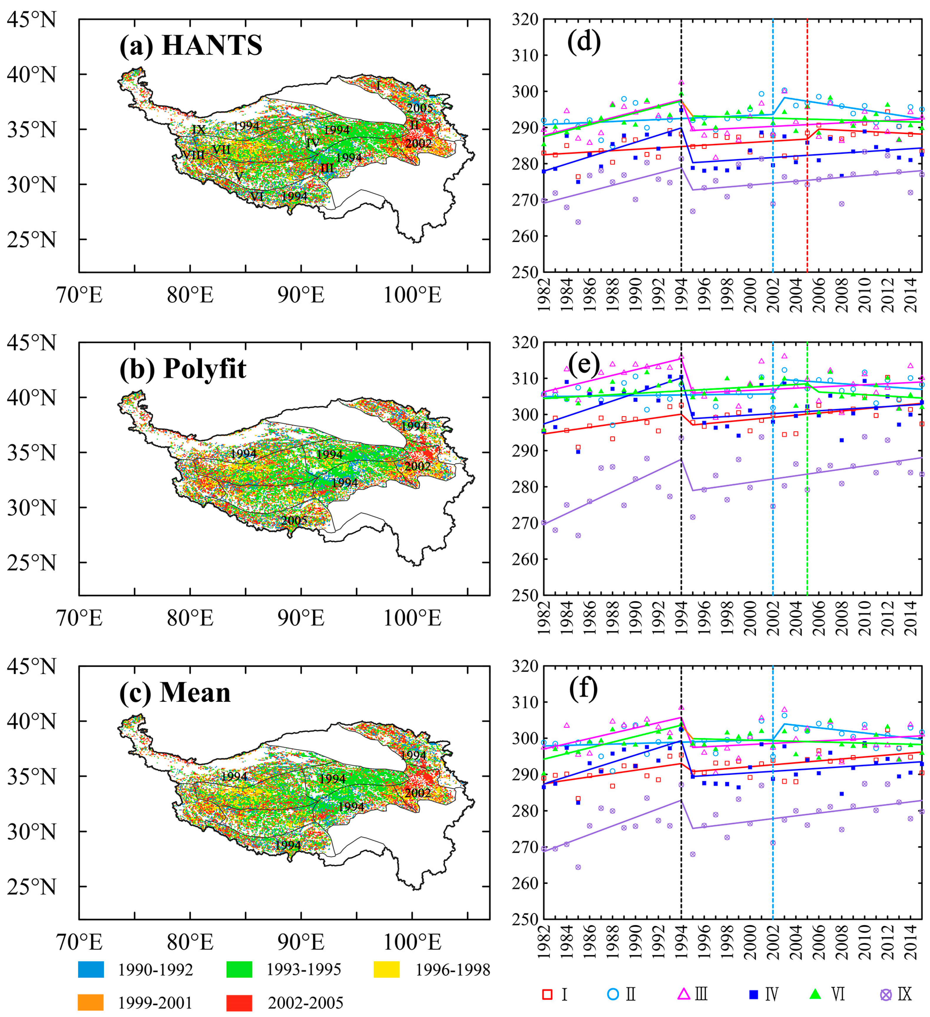
3.2. Detection of EOS Turning Points in the Subregions
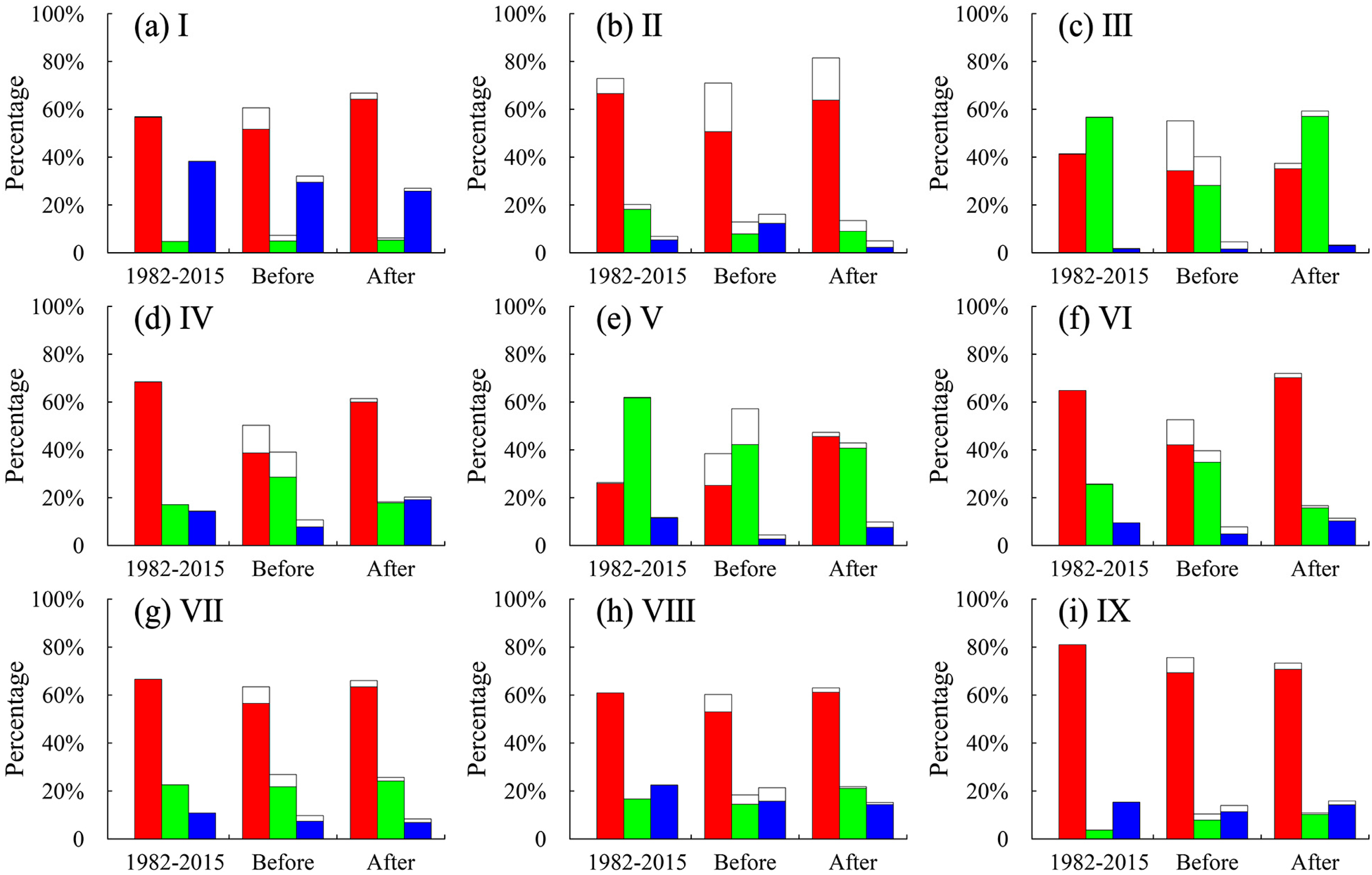
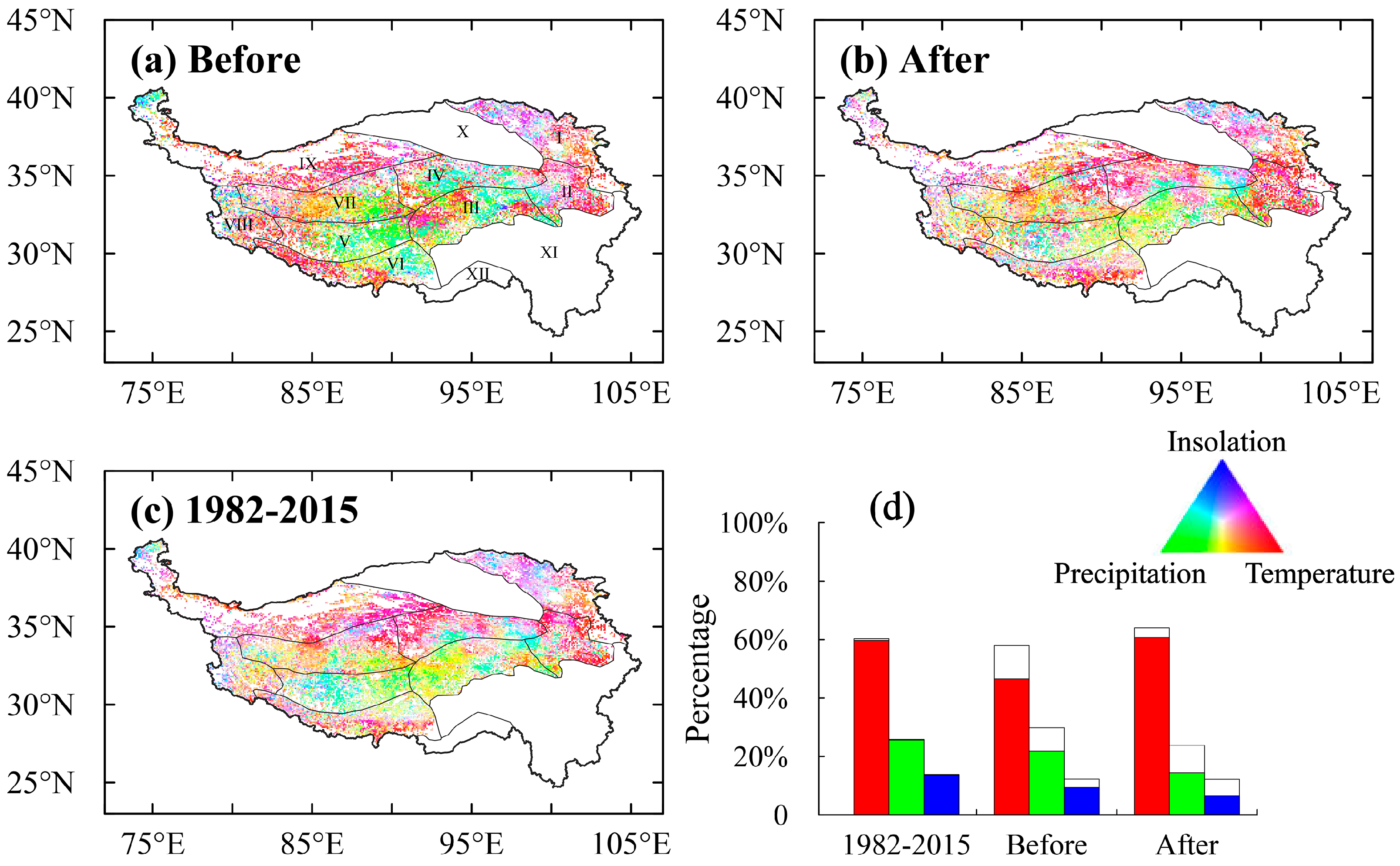
3.3. EOS Variations Controlled by Climatic Variables before and after Turning Points
3.4. Controls on the EOS Turning Points
4. Discussion
4.1. Controls on the EOS and EOS Turning Points
4.2. Ecological Significance of the EOS and Its Turning Points
4.3. Uncertainties, Challenges, and Future Directions
5. Conclusions
Author Contributions
Funding
Informed Consent Statement
Data Availability Statement
Conflicts of Interest
Appendix A
References
- Lieth, H. Phenology and Seasonality Modeling; Springer Science & Business Media: New York, NY, USA, 1974; Volume 8. [Google Scholar]
- Wang, J.; Sun, H.; Xiong, J.; He, D.; Cheng, W.; Ye, C.; Yong, Z.; Huang, X. Dynamics and drivers of vegetation phenology in three-river headwaters region based on the Google Earth engine. Remote Sens. 2021, 13, 2528. [Google Scholar] [CrossRef]
- Qiao, C.; Shen, S.; Cheng, C.; Wu, J.; Jia, D.; Song, C. Vegetation Phenology in the Qilian Mountains and its response to temperature from 1982 to 2014. Remote Sens. 2021, 13, 286. [Google Scholar] [CrossRef]
- Bornez, K.; Richardson, A.D.; Verger, A.; Descals, A.; Penuelas, J. Evaluation of vegetation and PROBA-V phenology using PhenoCam and Eddy covariance data. Remote Sens. 2020, 12, 3077. [Google Scholar] [CrossRef]
- Wang, S.Y.; Zhang, B.; Yang, Q.C.; Chen, G.S.; Yang, B.J.; Lu, L.L.; Shen, M.; Peng, Y.Y. Responses of net primary productivity to phenological dynamics in the Tibetan Plateau, China. Agric. For. Meteorol. 2017, 232, 235–246. [Google Scholar] [CrossRef]
- An, S.; Chen, X.Q.; Zhang, X.Y.; Lang, W.G.; Ren, S.L.; Xu, L. Precipitation and minimum temperature are primary climatic controls of alpine grassland autumn phenology on the Qinghai-Tibet plateau. Remote Sens. 2020, 12, 431. [Google Scholar] [CrossRef] [Green Version]
- Gonsamo, A.; Chen, J.M.; Ooi, Y.W. Peak season plant activity shift towards spring is reflected by increasing carbon uptake by extratropical ecosystems. Glob. Chang. Biol. 2018, 24, 2117–2128. [Google Scholar] [CrossRef]
- Li, X.T.; Guo, W.; Li, S.H.; Zhang, J.Z.; Ni, X.N. The different impacts of the daytime and nighttime land surface temperatures on the alpine grassland phenology. Ecosphere 2021, 12, e03578. [Google Scholar] [CrossRef]
- Lehikoinen, A.; Lindén, A.; Karlsson, M.; Andersson, A.; Crewe, T.L.; Dunn, E.H.; Gregory, G.; Karlsson, L.; Kristiansen, V.; Mackenzie, S.; et al. Phenology of the avian spring migratory passage in Europe and North America: Asymmetric advancement in time and increase in duration. Ecol. Indic. 2019, 101, 985–991. [Google Scholar] [CrossRef]
- Zhu, W.Q.; Tian, H.Q.; Xu, X.F.; Pan, Y.Z.; Chen, G.S.; Lin, W.P. Extension of the growing season due to delayed autumn over mid and high latitudes in North America during 1982–2006. Glob. Ecol. Biogeogr. 2012, 21, 260–271. [Google Scholar] [CrossRef]
- Bao, G.; Tuya, A.; Bayarsaikhan, S.; Dorjsuren, A.; Mandakh, U.; Bao, Y.H.; Li, C.L.; Vanchindorj, B. Variations and climate constraints of terrestrial net primary productivity over Mongolia. Quat. Int. 2020, 537, 112–125. [Google Scholar] [CrossRef]
- Wu, C.; Gough, C.M.; Chen, J.M.; Gonsamo, A. Evidence of autumn phenology control on annual net ecosystem productivity in two temperate deciduous forests. Ecol. Eng. 2013, 60, 88–95. [Google Scholar] [CrossRef]
- Sarvia, F.; De Petris, S.; Borgogno-Mondino, E. Exploring climate change effects on vegetation phenology by MOD13Q1 data: The piemonte region case study in the period 2001–2019. Agronomy 2021, 11, 555. [Google Scholar] [CrossRef]
- Richardson, A.D.; Keenan, T.F.; Migliavacca, M.; Ryu, Y.; Sonnentag, O.; Toomey, M. Climate change, phenology, and phenological control of vegetation feedbacks to the climate system. Agric. For. Meteorol. 2013, 169, 156–173. [Google Scholar] [CrossRef]
- Cheng, M.; Jin, J.X.; Jiang, H. Strong impacts of autumn phenology on grassland ecosystem water use efficiency on the Tibetan Plateau. Ecol. Indic. 2021, 126, 107682. [Google Scholar] [CrossRef]
- Dong, M.; Jiang, Y.; Zheng, C.; Zhang, D. Trends in the thermal growing season throughout the Tibetan Plateau during 1960–2009. Agric. For. Meteorol. 2012, 166–167, 201–206. [Google Scholar] [CrossRef]
- Shen, M.G.; Piao, S.L.; Dorji, T.; Liu, Q.; Cong, N.; Chen, X.Q.; An, S.; Wang, S.P.; Wang, T.; Zhang, G.X. Plant phenological responses to climate change on the Tibetan Plateau: Research status and challenges. Natl. Sci. Rev. 2015, 2, 454–467. [Google Scholar] [CrossRef] [Green Version]
- Chen, X.Q.; An, S.; Inouye, D.W.; Schwartz, M.D. Temperature and snowfall trigger alpine vegetation green-up on the world’s roof. Glob. Chang. Biol. 2015, 21, 3635–3646. [Google Scholar] [CrossRef]
- Zhang, G.; Zhang, Y.; Dong, J.; Xiao, X. Green-up dates in the Tibetan Plateau have continuously advanced from 1982 to 2011. Proc. Natl. Acad. Sci. USA 2013, 110, 4309–4314. [Google Scholar] [CrossRef] [Green Version]
- Li, P.; Peng, C.; Wang, M.; Luo, Y.; Li, M.; Zhang, K.; Zhang, D.; Zhu, Q. Dynamics of vegetation autumn phenology and its response to multiple environmental factors from 1982 to 2012 on Qinghai-Tibetan Plateau in China. Sci. Total Environ. 2018, 637–638, 855–864. [Google Scholar] [CrossRef]
- Fu, Y.S.H.; Campioli, M.; Vitasse, Y.; De Boeck, H.J.; Van den Berge, J.; AbdElgawad, H.; Asard, H.; Piao, S.; Deckmyn, G.; Janssens, I.A. Variation in leaf flushing date influences autumnal senescence and next year’s flushing date in two temperate tree species. Proc. Natl. Acad. Sci. USA 2014, 111, 7355–7360. [Google Scholar] [CrossRef] [Green Version]
- Peng, J.; Wu, C.Y.; Wang, X.Y.; Lu, L.L. Spring phenology outweighed climate change in determining autumn phenology on the Tibetan Plateau. Int. J. Climatol. 2021, 41, 3725–3742. [Google Scholar] [CrossRef]
- Cheng, M.; Jin, J.X.; Zhang, J.M.; Jiang, H.; Wang, R.Z. Effect of climate change on vegetation phenology of different land-cover types on the Tibetan Plateau. Int. J. Remote Sens. 2018, 39, 470–487. [Google Scholar] [CrossRef]
- Chen, J.; Yan, F.; Lu, Q. Spatiotemporal Variation of Vegetation on the Qinghai–Tibet Plateau and the Influence of Climatic Factors and Human Activities on Vegetation Trend (2000–2019). Remote Sens. 2020, 12, 3150. [Google Scholar] [CrossRef]
- Huang, K.; Zhang, Y.; Zhu, J.; Liu, Y.; Zu, J.; Zhang, J. The Influences of Climate Change and Human Activities on Vegetation Dynamics in the Qinghai-Tibet Plateau. Remote Sens. 2016, 8, 876. [Google Scholar] [CrossRef] [Green Version]
- Horion, S.; Prishchepov, A.V.; Verbesselt, J.; de Beurs, K.; Tagesson, T.; Fensholt, R. Revealing turning points in ecosystem functioning over the Northern Eurasian agricultural frontier. Glob. Chang. Biol. 2016, 22, 2801–2817. [Google Scholar] [CrossRef]
- Li, P.; Liu, Z.; Zhou, X.; Xie, B.; Li, Z.; Luo, Y.; Zhu, Q.; Peng, C. Combined control of multiple extreme climate stressors on autumn vegetation phenology on the Tibetan Plateau under past and future climate change. Agric. For. Meteorol. 2021, 308–309, 108571. [Google Scholar] [CrossRef]
- Siegmund, J.F.; Wiedermann, M.; Donges, J.F.; Donner, R.V. Impact of temperature and precipitation extremes on the flowering dates of four German wildlife shrub species. Biogeosciences 2016, 13, 5541–5555. [Google Scholar] [CrossRef] [Green Version]
- Bao, G.; Jin, H.; Tong, S.; Chen, J.; Huang, X.; Bao, Y.; Shao, C.; Mandakh, U.; Chopping, M.; Du, L. Autumn Phenology and Its Covariation with Climate, Spring Phenology and Annual Peak Growth on the Mongolian Plateau. Agric. For. Meteorol. 2021, 298–299, 108312. [Google Scholar] [CrossRef]
- Zheng, D. The Systematic Study of Ecogeographical Regions in China; Commercial Press: Beijing, China, 2008. [Google Scholar]
- Editorial Committee of Chinese Vegetation Map. Vegetation Map of the People’s Republic of China (1:1000000); Geological Publishing House: Beijing, China, 2006. [Google Scholar]
- Pinzon, J.E.; Tucker, C.J. A Non-Stationary 1981–2012 AVHRR NDVI3g Time Series. Remote Sens. 2014, 6, 6929–6960. [Google Scholar] [CrossRef] [Green Version]
- Deng, G.R.; Zhang, H.Y.; Yang, L.B.; Zhao, J.J.; Guo, X.Y.; Hong, Y.; Wu, R.H.; Dan, G. Estimating Frost during Growing Season and Its Impact on the Velocity of Vegetation Greenup and Withering in Northeast China. Remote Sens. 2020, 12, 1355. [Google Scholar] [CrossRef]
- Wu, J.H.; Liang, S.L. Assessing Terrestrial Ecosystem Resilience using Satellite Leaf Area Index. Remote Sens. 2020, 12, 595. [Google Scholar] [CrossRef] [Green Version]
- Wang, X.F.; Xiao, J.F.; Li, X.; Cheng, G.D.; Ma, M.G.; Zhu, G.F.; Arain, M.A.; Black, T.A.; Jassal, R.S. No trends in spring and autumn phenology during the global warming hiatus. Nat. Commun. 2019, 10, 10. [Google Scholar] [CrossRef]
- Shen, M.G.; Sun, Z.Z.; Wang, S.P.; Zhang, G.X.; Kong, W.D.; Chen, A.P.; Piao, S.L. No evidence of continuously advanced green-up dates in the Tibetan Plateau over the last decade. Proc. Natl. Acad. Sci. USA 2013, 110, E2329. [Google Scholar] [CrossRef] [Green Version]
- He, J.; Yang, K. China meteorological forcing dataset (1979–2015). In A Big Earth Data Platform for Three Poles: 2016; Northwest Institute of Eco-Environment and Resources: Lanzhou, China, 2016. [Google Scholar]
- Jakubauskas, M.E.; Legates, D.R.; Kastens, J.H. Harmonic analysis of time-series AVHRR NDVI data. Photogramm. Eng. Remote Sens. 2001, 67, 461–470. [Google Scholar]
- Piao, S.L.; Fang, J.Y.; Zhou, L.M.; Ciais, P.; Zhu, B. Variations in satellite-derived phenology in China’s temperate vegetation. Glob. Chang. Biol. 2006, 12, 672–685. [Google Scholar] [CrossRef]
- Liu, Q.; Fu, Y.S.H.; Zeng, Z.Z.; Huang, M.T.; Li, X.R.; Piao, S.L. Temperature, precipitation, and insolation effects on autumn vegetation phenology in temperate China. Glob. Chang. Biol. 2016, 22, 644–655. [Google Scholar] [CrossRef]
- Stow, D.; Daeschner, S.; Hope, A.; Douglas, D.; Petersen, A.; Myneni, R.; Zhou, L.; Oechel, W. Variability of the seasonally integrated normalized difference vegetation index across the north slope of Alaska in the 1990s. Int. J. Remote Sens. 2003, 24, 1111–1117. [Google Scholar] [CrossRef]
- Toms, J.D.; Lesperance, M.L. Piecewise regression: A tool for identifying ecological thresholds. Ecology 2003, 84, 2034–2041. [Google Scholar] [CrossRef]
- Yu, H.; Luedeling, E.; Xu, J. Winter and spring warming result in delayed spring phenology on the Tibetan Plateau. Proc. Natl. Acad. Sci. USA 2010, 107, 22151–22156. [Google Scholar] [CrossRef] [Green Version]
- Piao, S.L.; Wang, X.H.; Ciais, P.; Zhu, B.; Wang, T.; Liu, J. Changes in satellite-derived vegetation growth trend in temperate and boreal Eurasia from 1982 to 2006. Glob. Chang. Biol. 2011, 17, 3228–3239. [Google Scholar] [CrossRef]
- Borcard, D.; Legendre, P.; Drapeau, P. Partialling out the spatial component of ecological variation. Ecology 1992, 73, 1045–1055. [Google Scholar] [CrossRef] [Green Version]
- Oksanen, J.B.F.; Kindt, R.; Legendre, P.; O’hara, R.; Simpson, G.; Solymos, P.; Stevens, M.; Wagner, H. Multivariate Analysis of Ecological Communities. Version 1. Available online: http://cran.rproject.org/package=vegan (accessed on 1 May 2021).
- Yang, Y.Z.; Wang, H.; Harrison, S.P.; Prentice, I.C.; Wright, I.J.; Peng, C.H.; Lin, G.H. Quantifying leaf-trait covariation and its controls across climates and biomes. New Phytol. 2019, 221, 155–168. [Google Scholar] [CrossRef] [Green Version]
- Yamaura, Y.; Blanchet, F.G.; Higa, M. Analyzing community structure subject to incomplete sampling: Hierarchical community model vs. canonical ordinations. Ecology 2019, 100, e02759. [Google Scholar] [CrossRef]
- Gill, A.L.; Gallinat, A.S.; Sanders-DeMott, R.; Rigden, A.J.; Gianotti, D.J.S.; Mantooth, J.A.; Templer, P.H. Changes in autumn senescence in northern hemisphere deciduous trees: A meta-analysis of autumn phenology studies. Ann. Bot. 2015, 116, 875–888. [Google Scholar] [CrossRef] [PubMed] [Green Version]
- Zhang, Y.; Commane, R.; Zhou, S.; Williams, A.P.; Gentine, P. Light limitation regulates the response of autumn terrestrial carbon uptake to warming. Nat. Clim. Chang. 2020, 10, 739–743. [Google Scholar] [CrossRef]
- Chen, H.; Zhu, Q.; Wu, N.; Wang, Y.; Peng, C.-H. Delayed spring phenology on the Tibetan Plateau may also be attributable to other factors than winter and spring warming. Proc. Natl. Acad. Sci. USA 2011, 108, E93. [Google Scholar] [CrossRef] [PubMed] [Green Version]
- Sun, J.; Liu, M.; Fu, B.; Kemp, D.; Zhao, W.; Liu, G.; Han, G.; Wilkes, A.; Lu, X.; Chen, Y.; et al. Reconsidering the efficiency of grazing exclusion using fences on the Tibetan Plateau. Sci. Bull. 2020, 65, 1405–1414. [Google Scholar] [CrossRef]
- Wu, G.-L.; Du, G.-Z.; Liu, Z.-H.; Thirgood, S. Effect of fencing and grazing on a Kobresia-dominated meadow in the Qinghai-Tibetan Plateau. Plant. Soil 2009, 319, 115–126. [Google Scholar] [CrossRef]
- Li, G.Y.; Jiang, C.H.; Cheng, T.; Bai, J. Grazing alters the phenology of alpine steppe by changing the surface physical environment on the northeast Qinghai-Tibet Plateau, China. J. Environ. Manag. 2019, 248, 109257. [Google Scholar] [CrossRef]
- Badingquiying; Smith, A.T.; Harris, R.B. Summer habitat use of plateau pikas (Ochotona curzoniae) in response to winter livestock grazing in the alpine steppe Qinghai-Tibetan Plateau. Arct. Antarct. Alp. Res. 2018, 50, e1447190. [Google Scholar] [CrossRef] [Green Version]
- CaraDonna, P.J.; Iler, A.M.; Inouye, D.W. Shifts in flowering phenology reshape a subalpine plant community. Proc. Natl. Acad. Sci. USA 2018, 115, E9993. [Google Scholar] [CrossRef] [Green Version]
- Visser, M.E.; Gienapp, P. Evolutionary and demographic consequences of phenological mismatches. Nat. Ecol. Evol. 2019, 3, 879–885. [Google Scholar] [CrossRef] [PubMed]
- Teufel, B.; Sushama, L.; Arora, V.K.; Verseghy, D. Impact of dynamic vegetation phenology on the simulated pan-Arctic land surface state. Clim. Dyn. 2019, 52, 373–388. [Google Scholar] [CrossRef]
- Jin, J.; Wang, Y.; Zhang, Z.; Magliulo, V.; Jiang, H.; Cheng, M. Phenology Plays an Important Role in the Regulation of Terrestrial Ecosystem Water-Use Efficiency in the Northern Hemisphere. Remote Sens. 2017, 9, 664. [Google Scholar] [CrossRef] [Green Version]
- Liu, Y.; Wu, C. Understanding the role of phenology and summer physiology in controlling net ecosystem production: A multiscale comparison of satellite, PhenoCam and eddy covariance data. Environ. Res. Lett. 2020, 15, 104086. [Google Scholar] [CrossRef]
- Palacio, S.; Maestro, M.; Montserrat-Marti, G. Seasonal dynamics of non-structural carbohydrates in two species of mediterranean sub-shrubs with different leaf phenology. Environ. Exp. Bot. 2007, 59, 34–42. [Google Scholar] [CrossRef]
- Peng, J.; Wu, C.Y.; Zhang, X.Y.; Ju, W.M.; Wang, X.Y.; Lu, L.L.; Liu, Y.B. Incorporating water availability into autumn phenological model improved China’s terrestrial gross primary productivity (GPP) simulation. Environ. Res. Lett. 2021, 16, 094012. [Google Scholar] [CrossRef]


| ID | Subregion Names | AGDD0 Means (°C) | MI Means | Main Provinces |
|---|---|---|---|---|
| I | Alpine temperate steppe of the Qinghai Lake Basin | 1311.45 | 0.62 | Qinghai, Gansu |
| II | Alpine meadow steppe on the Zoige Plateau | 981.29 | 1.01 | Qinghai, Sichuan |
| III | Alpine meadow steppe on the Yushu-Naqu Plateau | 670.04 | 0.91 | Qinghai, Tibet |
| IV | Alpine meadow steppe on the sources of the Yangtze and Yellow rivers | 496.14 | 0.57 | Qinghai |
| V | Alpine and cold grassland on the Southern Chang Tang Plateau | 824.56 | 0.45 | Tibet |
| VI | Alpine temperate grassland of the Brahmaputra River Basin | 917.33 | 0.59 | Tibet |
| VII | Alpine and cold grassland on the Northern Chang Tang Plateau | 618.61 | 0.38 | Tibet |
| VIII | Alpine and cold grassland on the Upper Indus River Basin | 827.01 | 0.24 | Tibet |
| IX | Alpine and cold desert grassland of the Kunlun Mountains | 571.07 | 0.35 | Tibet, Xinjiang |
| X | Alpine desert in the Qaidam Basin | 1699.63 | 0.18 | Qinghai |
| XI | Alpine forestland in the Hengduan Mountain | 2043.25 | 1.14 | Sichuan, Yunnan |
| XII | Subtropical forestland in the southern Tibet | 3941.97 | 1.86 | Tibet |
| The EOS Turning Points versus Climate Turning Points | R2 | p Value |
|---|---|---|
| EOS~temperature | 0.331 | <0.01 |
| EOS~precipitation | 0.378 | <0.01 |
| EOS~insolation | 0.038 | 0.76 |
| Provinces | Climate Independent (%) | Human Activities Independent (%) | Climate-Human Activities Intersections (%) |
|---|---|---|---|
| Qinghai | 40.22 | 10.45 | 28.19 |
| Tibet | 66.17 | 6.80 | 9.98 |
Publisher’s Note: MDPI stays neutral with regard to jurisdictional claims in published maps and institutional affiliations. |
© 2021 by the authors. Licensee MDPI, Basel, Switzerland. This article is an open access article distributed under the terms and conditions of the Creative Commons Attribution (CC BY) license (https://creativecommons.org/licenses/by/4.0/).
Share and Cite
Yang, Y.; Qi, N.; Zhao, J.; Meng, N.; Lu, Z.; Wang, X.; Kang, L.; Wang, B.; Li, R.; Ma, J.; et al. Detecting the Turning Points of Grassland Autumn Phenology on the Qinghai-Tibetan Plateau: Spatial Heterogeneity and Controls. Remote Sens. 2021, 13, 4797. https://doi.org/10.3390/rs13234797
Yang Y, Qi N, Zhao J, Meng N, Lu Z, Wang X, Kang L, Wang B, Li R, Ma J, et al. Detecting the Turning Points of Grassland Autumn Phenology on the Qinghai-Tibetan Plateau: Spatial Heterogeneity and Controls. Remote Sensing. 2021; 13(23):4797. https://doi.org/10.3390/rs13234797
Chicago/Turabian StyleYang, Yanzheng, Ning Qi, Jun Zhao, Nan Meng, Zijian Lu, Xuezhi Wang, Le Kang, Boheng Wang, Ruonan Li, Jinfeng Ma, and et al. 2021. "Detecting the Turning Points of Grassland Autumn Phenology on the Qinghai-Tibetan Plateau: Spatial Heterogeneity and Controls" Remote Sensing 13, no. 23: 4797. https://doi.org/10.3390/rs13234797
APA StyleYang, Y., Qi, N., Zhao, J., Meng, N., Lu, Z., Wang, X., Kang, L., Wang, B., Li, R., Ma, J., & Zheng, H. (2021). Detecting the Turning Points of Grassland Autumn Phenology on the Qinghai-Tibetan Plateau: Spatial Heterogeneity and Controls. Remote Sensing, 13(23), 4797. https://doi.org/10.3390/rs13234797