Abstract
The total suspended solid (TSS) concentration (mg/L) is an important parameter of water quality in coastal waters. It is of great significance to monitor the spatiotemporal distribution and variation of TSS as well as its influencing factors. In this study, a quantitative retrieval model of TSS in Jiaozhou Bay (JZB) was established based on Landsat images from 1984 to 2020 (coefficient of determination (R2) = 0.77, root mean square error (RMSE) = 1.82 mg/L). In this paper, first, the long-term spatiotemporal variation of TSSs in JZB is revealed and, next, its influencing factors are further analyzed. The results show that the annual average TSSs in JZB reached their highest level in 1993 and their lowest level in 2016, showing a decreasing trend during the past decades. The TSSs were high in spring and winter and low in summer and autumn. The spatial distribution of the TSSs in JZB was similar at different timepoints, i.e., high in the northwest and gradually decreasing to the southeast. Tidal elevation exerted a significant influence on the daily variation of TSSs, and wind speed had a significant influence on the seasonal variation of TSSs. The Dagu River’s discharge only affected the TSSs at the river mouth. Tidal elevation, river discharge, and wind speed were major influence factors for TSSs’ variation in JZB. The results showed that the empirical model based on Landsat satellite data could be used to effectively monitor the long-term variation of TSSs in JZB.
1. Introduction
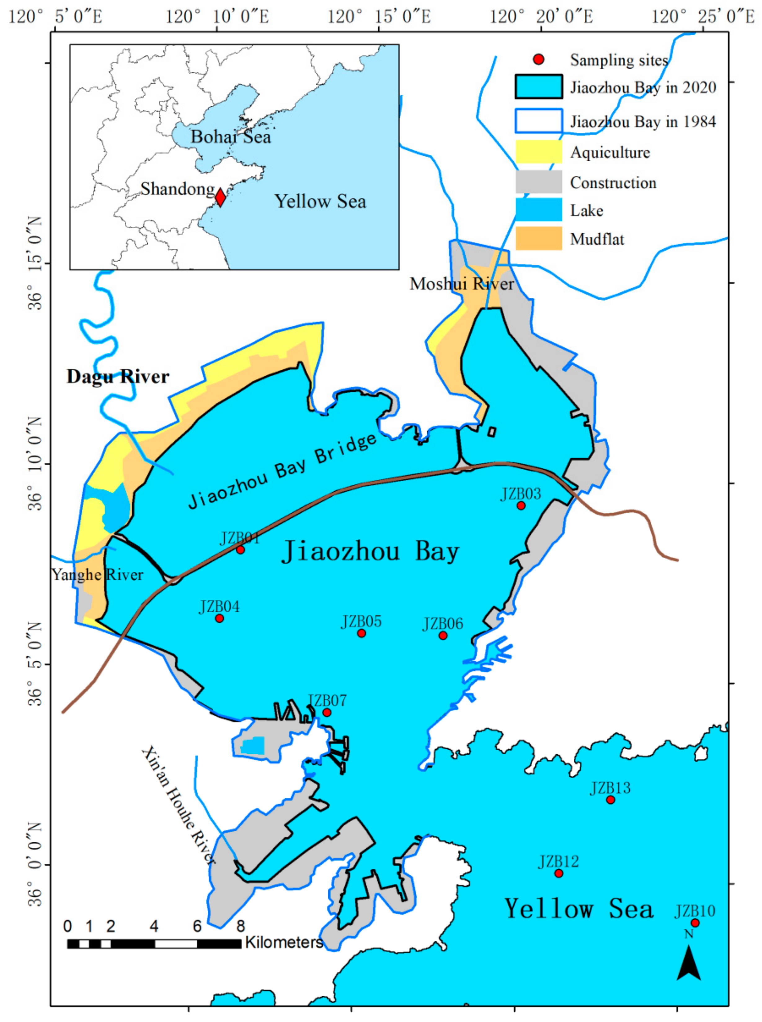
Jiaozhou Bay (JZB) (35°38′–36°18′N, 120°04′–120°23′E) is a semi-enclosed bay on the south coast of the Shandong Peninsula, China. It is located between the Shinan and Huangdao regions of Qingdao City, with a trumpet-shaped exit connected to the Yellow Sea (Figure 1). JZB covers an area of nearly 500 km2, with a narrow entrance, deep channels, low turbidity, weak tides, and low sea waves. As a natural port, it promotes the development of the transportation industry of Qingdao [1]. Bounded by the southern end of Tuandao and the northern end of Xuejiadao, the bay mouth is about 2.5 km wide. JZB is about 27.8 km wide from east to west and 33.3 km long from north to south. The coastline is about 163 km long, and the tidal flat area is about 125 km2. However, with the process of urbanization of Qingdao City, the area and coastline length of JZB are decreasing and the total suspended solid (TSS) concentration is also changing [2].
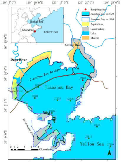
Figure 1.
Location of Jiaozhou Bay (the blue line is the boundary of JZB in 1984, the black line represents the boundary of JZB in 2020; the red dots are the location of the sampling sites).
As one of the important parameters of coastal and inland water environmental quality, the study of TSSs is of great significance. On the one hand, TSSs play an important role in the indication of pollution levels and the accurate estimation of soil erosion; on the other hand, TSSs reduce the light energy entering the water body, affect the growth of aquatic plants, and control the primary productivity of phytoplankton [3]. The TSSs in JZB have always been a concern for scientists and managers. Zhang et al. [4] studied the spatial distribution and seasonal variation of TSSs in JZB from 1994 to 1998 using field-measured data, and studied the main influencing factors of TSS. Bi et al. [5] used flow cytometry and other methods to study the distribution characteristics and influencing factors of suspended particulates of JZB in summer. Although the traditional field measurement method can reveal accurate information for a specific location, it is time-consuming and labor-intensive, and cannot reflect the temporal and spatial distributions of TSSs. Remote sensing technology, as an alternative, is time-saving, cost-effective, and highly efficient. It can be used to ascertain the distribution of the TSS concentration on a large scale, and offers better spatial and temporal resolution than the traditional methods. With these advantages in mind, previous studies have proposed many remote sensing retrieval methods for TSS monitoring. The empirical algorithm is simple in form and convenient in application, and has been proposed and widely used. Yu et al. [6] established an empirical algorithm retrieval model to study the TSSs in the Yellow Sea based on Moderate Resolution Imaging Spectroradiometer (MODIS) data, and analyzed the overall distribution characteristics and seasonal variation of the TSSs. To improve on the accuracy of this approach, some studies have also used semi-analytical algorithms that combine empirical equations, radiation transmission models, and bio-optical models. Zhang et al. [7] established a semi-analytical algorithm for studying the TSSs in the Yellow Sea and East China Sea based on MODIS satellite data and field-measured data. Hou et al. [8] constructed a semi-analytical model of the TSSs in JZB based on the data from three different satellites, along with the field-measured data from 2001 to 2015.
Due to the difficulty of obtaining physical parameters for semi-analytical algorithms, empirical models are most widely used in operational monitoring. Moreover, the small area of JZB means that the coarse spatial resolutions of Medium Resolution Imaging Spectrometer (MERIS) or MODIS cannot reflect the subtle variations in the TSS distribution. In addition, there are few studies focusing on the long-term spatiotemporal variation of TSSs in JZB or the important influencing factors. Therefore, in this study, a quantitative retrieval model for studying the TSSs in JZB was established based on field-measured data and remote sensing data from 1984 to 2020, and the spatiotemporal distribution and variation of TSSs in JZB were revealed and analyzed. Moreover, tidal, wind, and Dagu River discharge data were used to quantitatively analyze the main influencing factors of TSS variation in JZB.
2. Materials and Methods
2.1. In-Situ Data
In this study, a total of 23 sets of field-measured data were obtained from the JZB Marine Ecosystem Research Station (http://jzw.qdio.cas.cn/ (accessed on 10 January 2021)). The concentration of TSS was measured following the gravimetric method. The water samples were first filtered through dried and pre-weighed 0.45 μm membranes. Next, the membranes were dried at 45 °C for 24 h before weighed. The process of drying was repeated until the difference of successive calculated TSS values was less than 0.01 mg/L. The data acquisition dates are shown in Table 1, and the location information for the sampling sites is shown in Figure 1.

Table 1.
Information of Sampling sites.
2.2. Acquisition and Preprocessing of Landsat Data
Landsat data were obtained from the Google Earth Engine (GEE) platform, including Theme Mapper (TM), Enhanced Theme Mapper Plus (ETM+), and Operating Land Imager (OLI). For quality control, images with cloudiness greater than 10% were excluded. Next, the Quality Assessment (QA) band algorithm was applied to detect and remove the clouds and cloud shadows on the remaining Landsat images. Finally, a total of 331 images from 1984 to 2020 were used for the remote sensing retrieval of TSSs in JZB. To reduce the reflectance differences caused by the three different sensors, the empirical line method [9] was used. Firstly, the linear relationship between the reflectance of OLI and TM/ETM+ images was established, and then the reflectance of the TM/ETM+ images was adjusted to the same level as the reflectance of the OLI images.
Because of the loss of data bands in the images acquired from Landsat7 ETM+ after 31 May 2003 [10], the focal mean function was used to fill the gap. The LEDAPS (Landsat Ecosystem Disturbance Adaptive Processing System) was used to perform atmospheric correction on Landsat TM and ETM+ images, and LaSRC (Landsat Land Surface Reflectance Code) was used to perform atmospheric correction on Landsat OLI images.
2.3. Acquisition and Preprocessing of GOCI Data
The Geostationary Ocean Color Imager (GOCI) takes observations eight times a day between 8:00 and 15:00 Beijing time [11]. To analyze the influence of tides on the TSSs of JZB, the TSS product of the GOCI was downloaded (http://kosc.kiost.ac.kr/index.nm (accessed on 12 May 2021)). The projection coordinate system of the GOCI TSS product was converted, in keeping with that of the Landsat images.
2.4. Other Data
The tidal data for JZB were obtained from the daily tide predictions of the Qingdao Dagang Station from 1986 to 2017 [12]. Numerical simulation is an important method with which to study the dynamic environment of the gulf, one that transcends the constraints of time and space. Since the periodic curve of the ocean tide level is similar to a sine curve, this study interpolated the predicted tidal data to simulate the tidal elevation at the time when remote sensing satellite images were captured.
The daily wind data from 1984 to 2017 were obtained from the National Meteorological Station of China. The main inflow rivers of JZB are 13 rivers including the Dagu, Moshui, Baisha, Yanghe, and Jiaolai. Dagu River is the largest among these rivers, accounting for about 50% of total discharge. [13]. Therefore, the monthly average Dagu River discharge data from the Nancun Hydrological Station [14] were used to analyze the influence of river discharge on the TSSs in JZB. The Nancun Hydrological Station is located at the lower reach of the Dagu River Basin and has a long-term discharge record from 1984 to 2013, which can illustrate the overall characteristics of the river basin’s discharge.
2.5. TSS Algorithm Development
Previous researchers have found that differences in water substances cause differences in water reflectance and ocean color, and that a multi-band combination model can reduce this effect [15]. The spectral reflectance ratio of two or more bands can also eliminate part of the influence caused by the refraction coefficient and backscatter of suspended sediments [16]. In addition, it can eliminate the product effect of atmospheric influence and surface noise, and thus emphasize the target information [17]. Therefore, the band ratio is more suitable for modeling than a single band.
We first conducted a waveband sensitivity analysis and found that the red band exhibited the highest correlation with the TSSs. Therefore, a combination of the red band and other bands was used as a remote sensing factor to analyze the correlation with the TSSs. Table 2 shows the correlations between eight band combinations and the TSSs, and the band combination with the highest correlation is (G + R)/(G/R) (G is the green band remote sensing reflectance, and R is the red band remote sensing reflectance). Therefore, this was used as an independent variable to establish a quantitative retrieval model of the TSSs.
Table 2.
Correlation analysis of band combination and TSS.
A reliable “leave-one-out cross-validation” uncertainty evaluation method was used to calibrate and verify the model, to minimize the influence of random factors [18]. Using all the pairs of remote sensing reflectance and TSS for modeling, and a pair of data for model verification, the coefficient of determination (R2) and root mean square error (RMSE) were calculated to determine the most accurate TSS retrieval model. The model with the best performance was as follows:
where X was (B2 + B3)/(B2/B3) for Landsat 5 and Landsat 7 and (B3 + B4)/(B3/B4) for , while Y was the TSSs. The B2, B3, and B4 are the reflectance associated with Landsat channels.
Y = 0.71 × exp(21.31X),
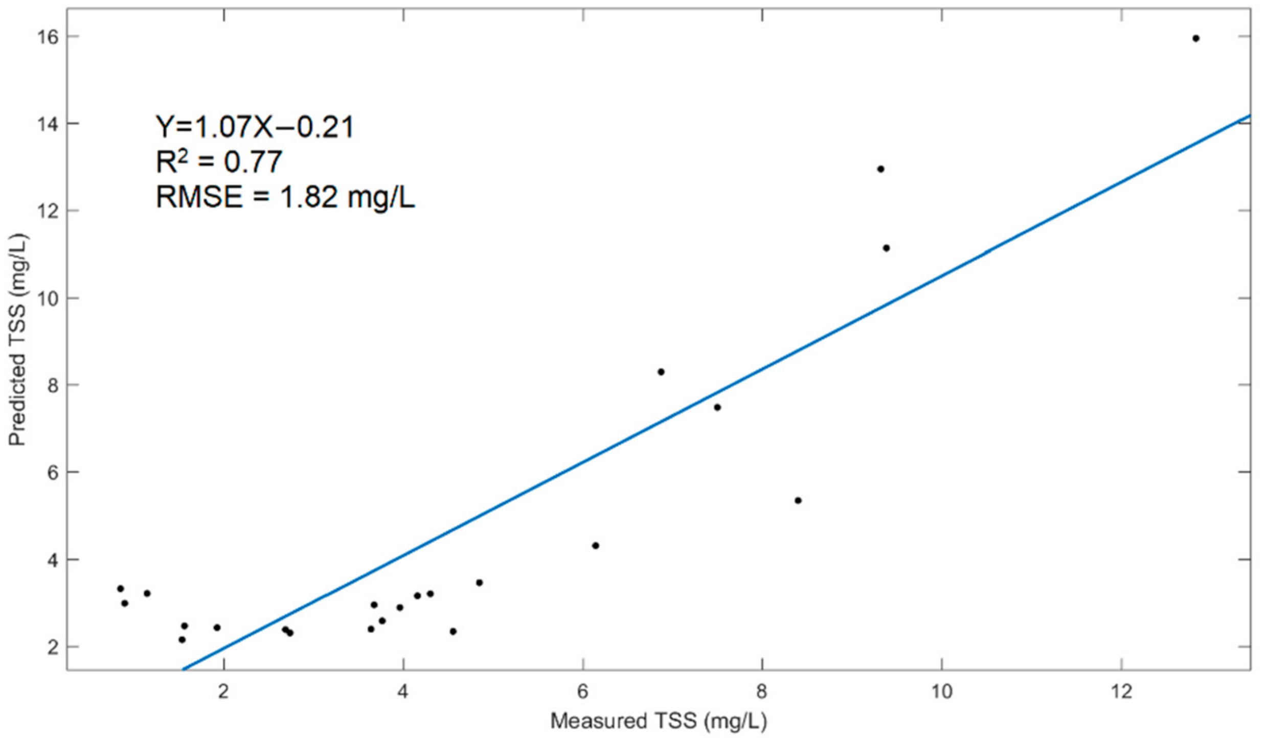
Figure 2 presents the validation of the proposed retrieve model. The model had high explanatory and predictive capabilities. The R2 was 0.77, the RMSE was 1.82 mg/L, and the slope of the trend line was 1.07. The scattered points were evenly distributed on both sides of the trend line, and all the predicted TSSs that fell within the field measurement range.
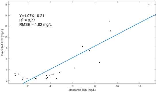
Figure 2.
Relationship between the measured and predicted TSS.
3. Results
3.1. Spatiotemporal Distribution of TSS
The spatiotemporal distribution of TSSs in JZB between 1984 and 2020 was first revealed from Landsat images using Equation (1). The TSSs of JZB varied in the range of 0–150 mg/L; they were higher in the northwest and gradually decreased to the southeast. The TSSs in the estuary and nearshore were mostly higher than 30 mg/L, and were below 30 mg/L in the center of the bay.
Figure 3 shows the variation of the annual average TSS retrieved from Landsat data between 1984 and 2020. The annual average TSSs fluctuated between 1984 and 2020. The TSSs reached a maximum in 1993 (26.94 mg/L) and dropped to a minimum (10.69 mg/L) in 2016, showing an overall downward trend, as described by Gao et al. [19].
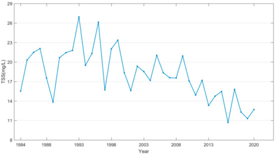
Figure 3.
Variation of the annual average TSS in JZB from 1984 to 2020.
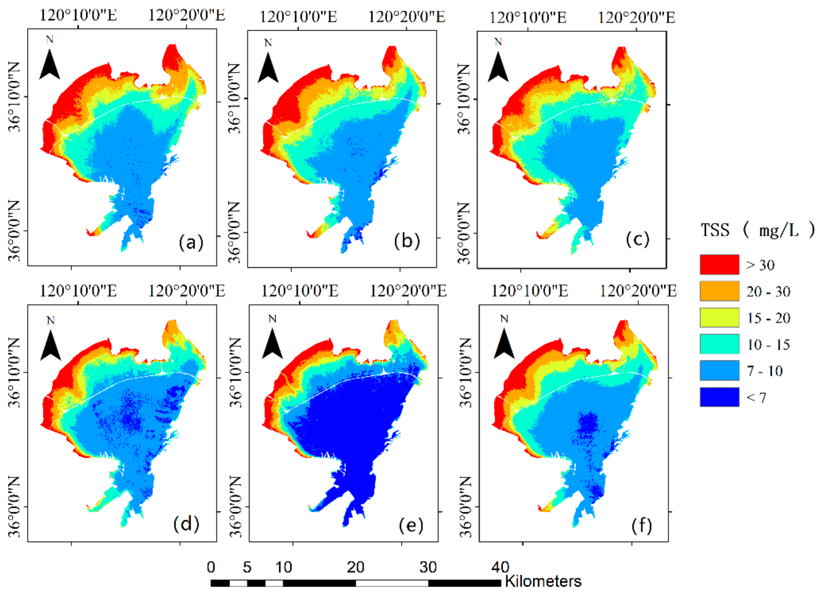
To analyze the variation in the TSS spatial distribution in JZB over the past 37 years, 331 scenes of images from 1984 to 2020 were divided into five periods, according to the period average method adopted by Li et al. [20]: (a) 1984–1995, (b) 1996–2001, (c) 2002–2008, (d) 2009–2015, and (e) 2016–2020.
These five periods were divided equally by the number of images to the greatest extent, but the time intervals were not equal. Using the average synthesis method, the average TSS map for each period and the total average TSS map for the five periods were calculated (Figure 4a–f). As shown in Figure 4a–e, the low TSS concentration range (<10 mg/L) expanded gradually in its spatial distribution, while the high TSS concentration range (>30 mg/L) in the north gradually decreased from period a to period e. Based on the image of each period, the overall distribution pattern of high TSSs near-shore and low TSSs far-shore was maintained. In general, the overall TSSs in JZB showed a downward trend; the highest value appeared in period a (16.53 mg/L) and the lowest value appeared in period e (11.03 mg/L), which was consistent with the spatial distribution trend.

Figure 4.
Variation of the average TSS in each period (a–e) is the average TSS for period (a) to period (e); (f) is the average TSS for five periods.
The spring (March, April, and May), summer (June, July, and August), autumn (September, October, and November), and winter (December, January, and February) average TSSs from 1984 to 2020 are shown in Figure 5. In general, the TSSs in JZB were relatively low, with obvious spatial and seasonal variations. The TSSs were high in spring and winter, and low in summer and autumn, reaching a maximum in spring (17.62 mg/L) and a minimum in summer (12.92 mg/L). From a spatial point of view, the distribution trend of the average TSSs in the four seasons was similar. The TSSs in the northwest of JZB were higher than in the southeast, and gradually decreased from the coast to the sea. The variation trend of the monthly average TSSs was consistent with the seasonal average TSSs. The monthly average TSSs first increased from January to May, then dropped to August, before rising to December. The highest TSSs appeared in May (23.32 mg/L) and the lowest appeared in August (9.71 mg/L).
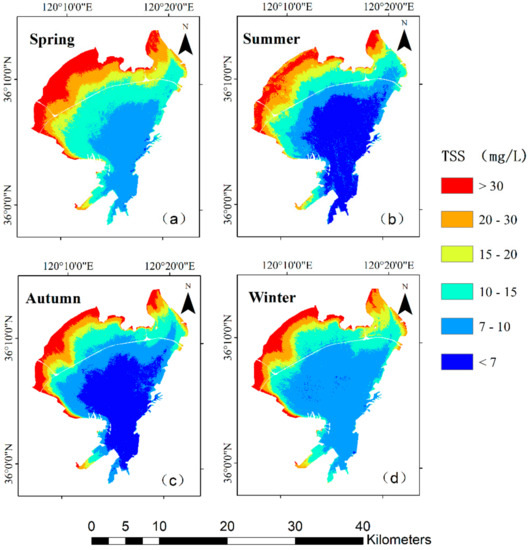
Figure 5.
Variations of the average TSS in each season (a–d) are average TSS in spring, summer, autumn, and winter, respectively).
3.2. Comparison of Landsat and GOCI
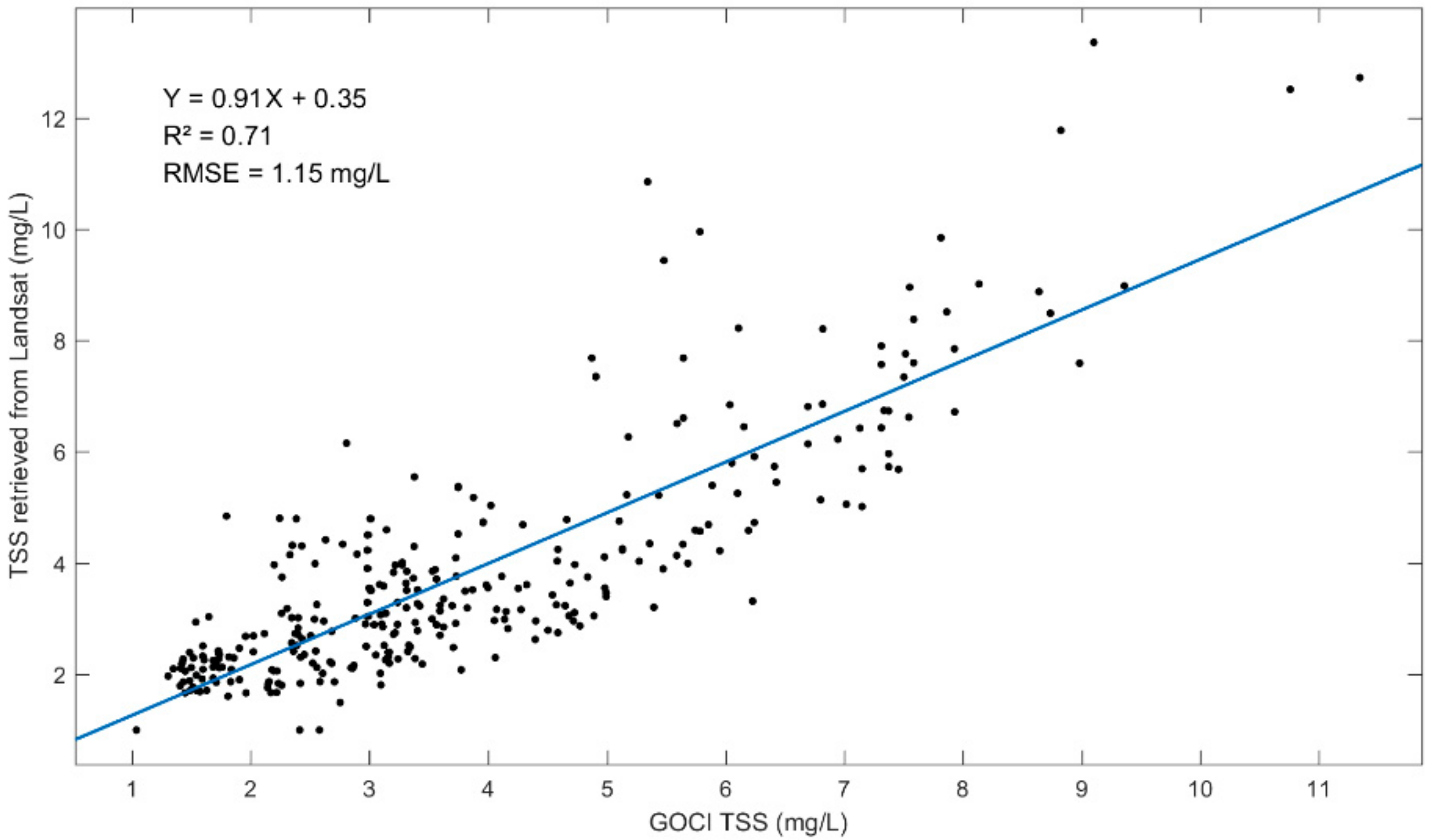
In this study, the influence of tides on the TSSs was analyzed with the TSS product of the GOCI. To evaluate the consistency between the TSS data from two different sensors, the TSSs retrieved from Landsat between 2011 and 2020 were compared with the GOCI TSS product for the corresponding dates. As shown in Figure 6, the slope of the trend line was 0.91, the R2 was 0.71, and the RMSE was 1.15 mg/L. Therefore, the TSS data from the GOCI and Landsat showed a good consistency, which afforded us the possibility of analyzing the influence of the tide on TSSs using high time-resolution GOCI TSS data.
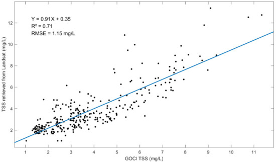
Figure 6.
Comparison between TSS data from GOCI and Landsat.
4. Discussion
4.1. Uncertainties
Due to the relatively low temporal resolution of Landsat and the limited number of field-measured data used in this study, there were differences between the acquisition time of field-measured data and of satellite data, which inevitably introduced uncertainties into the retrieval model as shown in verification in Figure 2. In addition, lack of in situ data collected close to the coast in JZB, the retrieval model was developed based on a limited TSS variation range upwards to 13 mg/L, but a fraction of TSS values spread well above 30 mg/L. This limited range of field measured data would also introduce uncertainties. Owing to the cloudy summer weather in JZB, there were fewer Landsat images available in summer compared to in other seasons. As a result, the temporal and spatial distribution characteristics revealed by the retrieval model may be somewhat different from the actual situation. Besides this, the northern coast of JZB was greatly affected by the high reflectance of sediments from shallow waters; therefore, the high TSSs in this area revealed by the retrieval model might be inconsistent with reality.
However, taking relatively high spatial resolution and a dataset of over 40 years into consideration, Landsat data were still suitable for monitoring the spatiotemporal variation of the TSSs in JZB. In addition, the spatiotemporal distribution and influencing factors of TSSs in JZB in this paper were consistent with the results of Zhang et al. [4], who used field-measured data. Therefore, the research results based on Landsat data could still reflect the subtle spatiotemporal variations of TSSs in JZB over the past 37 years.
4.2. Dominant Drivers of TSS
According to the results (Section 3), the TSSs of JZB are generally low, and there are obvious spatiotemporal variations. The annual average TSSs in JZB showed a downward trend as a whole due to reduced tidal currents with the process of land reclamation over the past decades [19]. The horizontal advection of TSSs associated with the horizontal gradient of the TSSs originally led net suspended sediment movement between JZB and the neighboring sea to be seaward. TSSs transport from the tidal flats were reduced with the tidal flats being reclaimed, and subsequently reversed direction after 1986 [19]. Land reclamation weakened tidal currents and the horizontal gradient of TSS [19], probably resulting in a decrease in the TSSs in JZB.
Many studies have shown that factors such as the tide, river discharge, and wind are the main influences on the variation of TSSs [21,22,23]. To better understand the reasons for the TSS variation, field-measured data and remote sensing data were applied to quantitatively and qualitatively analyze the effects of different factors on the TSSs.
The tides of JZB are semi-diurnal, and the tidal current spreads along the inner channel of the bay to reach the top of the bay. The velocity of flood tidal current is greater than that of ebb tidal current [24]. The velocity at the mouth of the bay is greater than that within the bay, which makes it easy for a small amount of sediment from outside of the bay to move into the bay. However, it is not conducive to the spread of material from within the bay to outside of the bay, especially not in the northern bay. Therefore, the TSSs gradually decrease from the top to the mouth of the bay. Because the shore water is shallow, the sea-bottom sediments are susceptible to waves and are suspended in the sea, so the TSSs in the shore water are relatively high [4].
Possible hydrodynamic or meteorological influencing factors of water-surface TSSs include the tidal current magnitude, tidal current direction, river discharge, wind speed, and wind direction. To qualitatively illustrate these different control factors, we selected pairs of images in which only one variable significantly varied (See Table 3). The sole influence of tidal current magnitude on TSSs—under similar conditions of tidal current direction, river discharge, and wind speed and direction—is shown in Figure 7a,b. The influences of tidal current direction (Figure 7d,e), river discharge (Figure 7g,h), wind speed (Figure 7j,k), and wind direction (Figure 7m,n) are also illustrated on TSS concentration maps. We used a section line from the northwest to the southeast of JZB to extract the TSSs along the line, in order to show the spatial variation of TSSs in JZB.
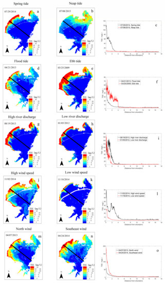
Figure 7.
Spatial distribution of TSSs under the control of a sole influence factor and variation of TSSs along the section line: tidal current magnitude (a–c); tidal current direction (d–f); river discharge (g–i); wind speed (j–l); wind direction (m–o) (The black line is the section line).
The TSSs near the shore during the spring tide were 2–10 times greater than those during the neap tide (Figure 7a–c). This is because the driving force of the spring tide was much greater than that of the neap tide, and the resuspension effect of the nearshore sediment was intense. Due to the decrease in the water level during the ebb tide, the high reflectance of the sediment in the coastal waters led to the high concentration of TSSs in the coastal waters (Figure 7e). The influx of clear water outside the bay during the flood tide resulted in a slight decrease in the TSSs in the bay (Figure 7d,f). The high river discharge caused 2–3 times more TSSs in the estuary than the low river discharge (Figure 7i). Compared to a slow wind speed (1.8 m/s on 18 November 2014), a fast wind speed (6.9 m/s of 2 November 2014) resulted in strong sea waves and increased TSSs, especially in shallow coastal waters (Figure 7j–l). The TSS concentration was also influenced by the monsoon climatic characteristics. As shown in Figure 7m,n, a southeastern wind caused more sediments to resuspend in the shallow coastal waters than a northern wind (Figure 7o), but in terms of the average TSSs, the difference between the two was not obvious. Therefore, the wind speed was a meteorological factor that affected the distribution of TSSs in JZB more than the wind direction.
4.2.1. Tide
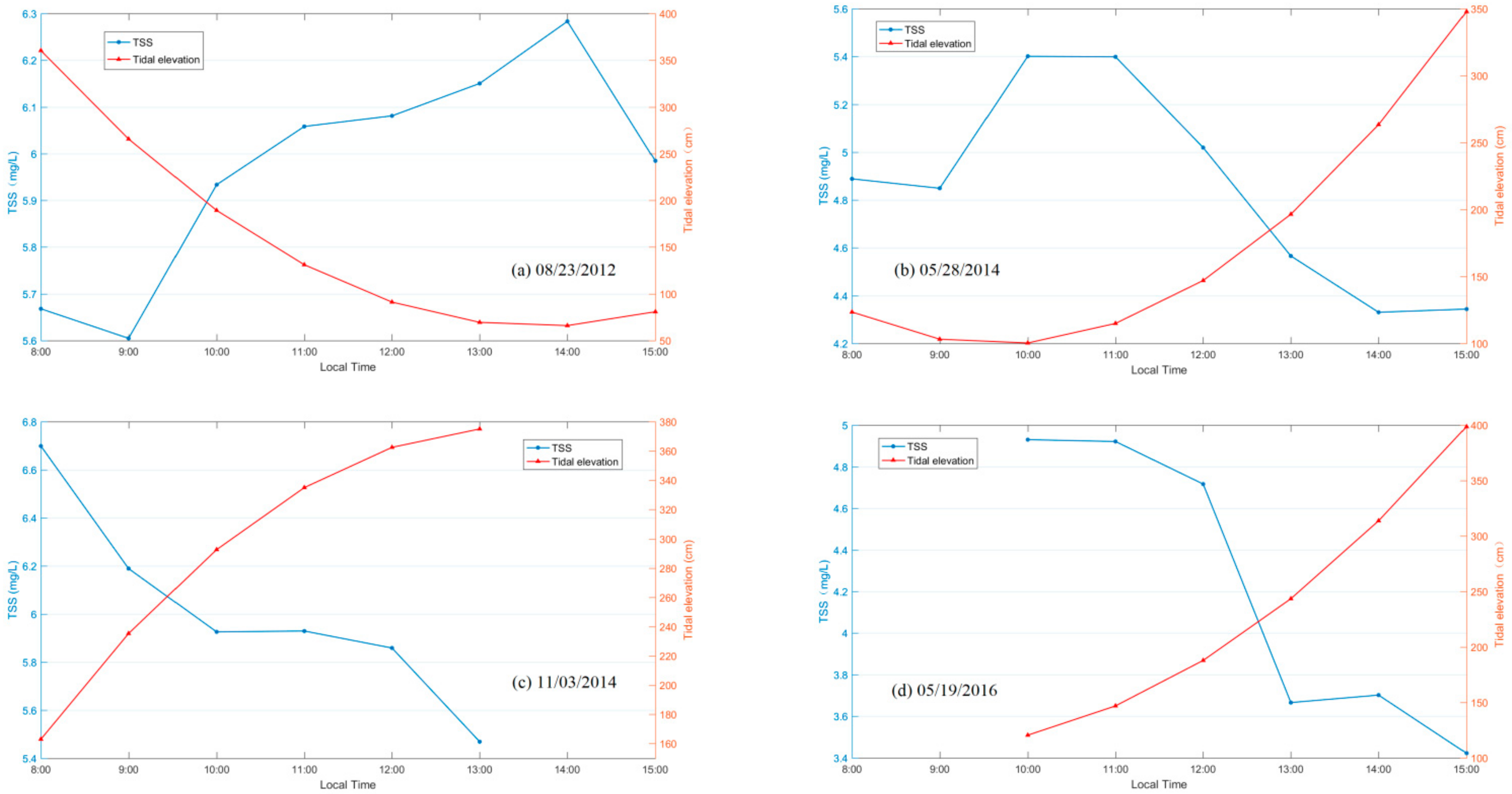
To further analyze the influence of the tide on the TSSs, we analyzed the relationship between Landsat-retrieved TSSs and tidal elevation (Figure 8). Generally speaking, tidal elevation explained approximately 25% of the overall variance of the TSSs, but there was little difference between flood and ebb tide (data no shown). Next, this result was further validated by analyzing the relationship between the variation of the average GOCI TSS data in JZB and the tidal elevation in a day. Taking 23 August 2012, 28 May 2014, 3 November 2014, and 19 May 2016 as examples (Figure 9), it can be seen that the TSSs were negatively correlated with the tidal elevation in a day. The higher the tidal elevation, the smaller the TSS. The TSS usually reached a minimum at high tide, owing to clear seawater in the open sea pouring into the bay. In comparison, the TSS reached its maximum at the ebb tide, on account of the intense resuspension of sediment in shallow water.
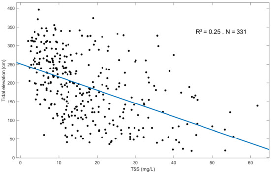
Figure 8.
The relationship between Landsat-retrieved TSSs and tidal elevation.
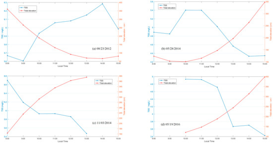
Figure 9.
Relationship between variation of GOCI TSS and tidal elevation during 8:00–15:00 a day (the blue line is the variation of TSS, and the red line is the variation of tidal elevation; (a) is 23 August 2012; (b) is 28 May 2014; (c) is 3 November 2014; (d) is 19 May 2016.
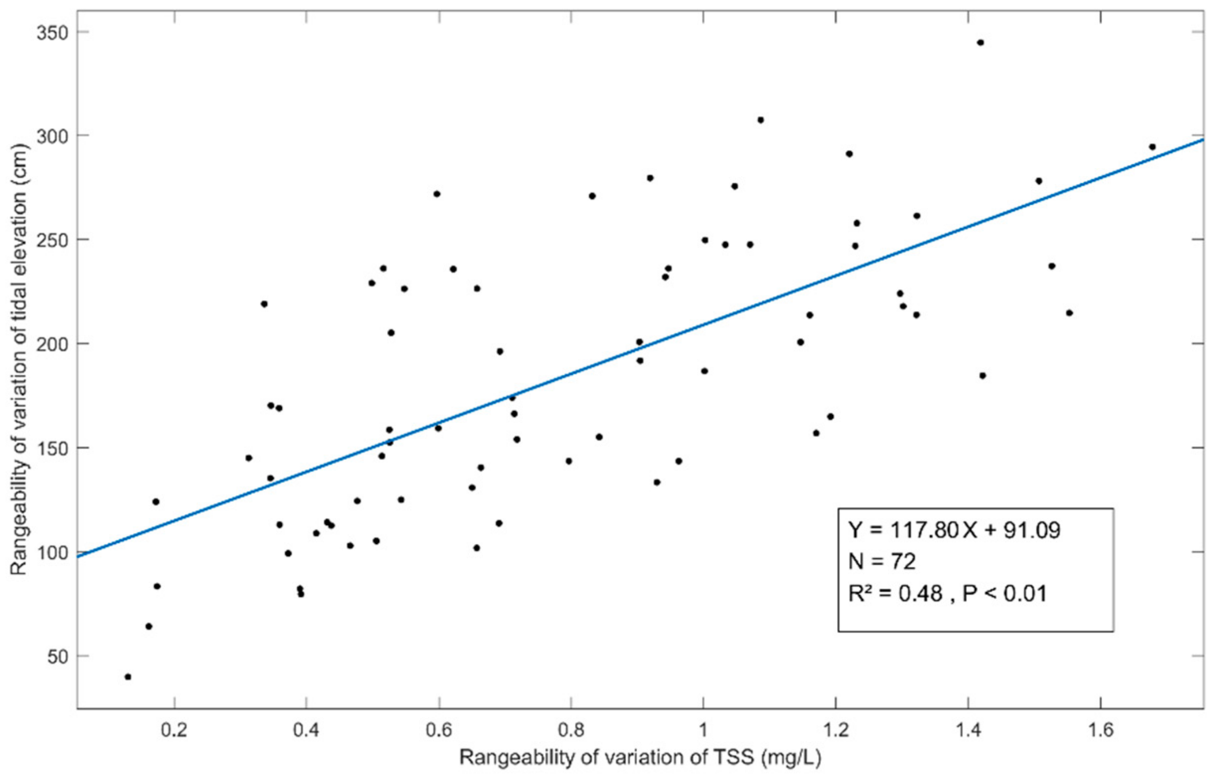
We analyzed the relationship between the rangeability of TSS concentration and the rangeability of tidal elevation in one day. In order to reduce the uncertainties caused by the small number of images, it was necessary to ensure that there were at least four available and integrated GOCI TSS images of JZB in one day, including high-tide or low-tide moments. As a result, only 72 days of GOCI TSS data were selected from all the available data. Next, the average GOCI TSS data were analyzed with corresponding tidal elevations. Figure 10 illustrates that there was a positive correlation between the rangeability of TSS concentration and tidal elevation within one day (R2 = 0.48). Therefore, the rangeability of tidal elevation in JZB affected the rangeability of the TSSs to a large extent.
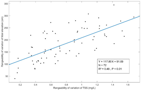
Figure 10.
Relationship between rangeability of variation in TSS concentration and rangeability of variation in tidal elevation in one day.
4.2.2. River Discharge
The influx of the river also creates more sediment [25]. A pixel-by-pixel correlation analysis between the monthly average TSSs and the monthly average discharge of Dagu River is shown in Figure 11. The correlation coefficient in the northwestern part of JZB was relatively high, and was low in the central bay. As the main water source of JZB, the impact of Dagu River discharge on the TSSs weakened quickly toward the central bay. In addition, there were several high-value areas, which are marked as A, B, C, D, and E in Figure 11. The high-value areas A and C were located at the mouth of the Moshui River and Yanghe River, respectively. The high correlation coefficient between the TSSs and the river discharge was due to the impact of the sediment injected by the two rivers. The high-value area B was close to the shore aquaculture area, and aquaculture activity might have caused resuspension and thus a high TSS concentration. The high-value areas D and E were near several logistics companies and Qingdao Bonded Port Logistics Park, respectively. They were influenced by human factors such as cargo ship passage. In addition, the area D was also affected by some aquaculture areas. However, the correlation coefficients near the Dagu River estuary and near-shore area were low. The shallow water near shore may explain these phenomena if the high reflectance of sediments led to continuously high TSSs in spite of obvious seasonal variation of river discharge. Further analysis revealed that the monthly river discharge could only explain 25% of the TSS variation (R2 = 0.25), indicating that when the river discharge was low, other factors controlled the TSS distribution and variation near this area.
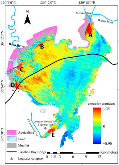
Figure 11.
Pixel-by-pixel correlation analysis between the monthly average TSSs and Dagu River discharge. The color bar indicates the value of Pearson’s correlation coefficient (r). A, B, C, D, and E are five high-value areas.
4.2.3. Wind
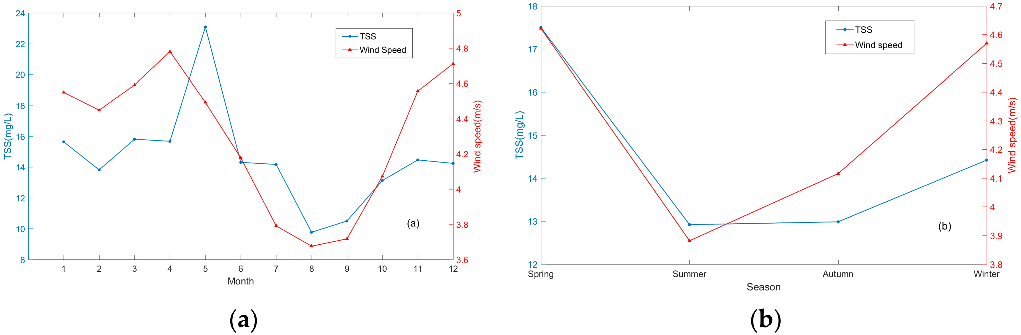
JZB is influenced by a temperate monsoon climate. With a southeastern wind dominating, JZB is windy in spring and winter, and the annual average wind speed is 5.4 m/s [26]. Strong winds cause more waves, and thus cause more sediment to resuspend [27]. The monthly and seasonal average wind speeds in JZB were calculated and compared with the monthly and seasonal average TSSs retrieved from the Landsat data (Figure 12). Wind speed showed obvious seasonality throughout the year. It increased first and reached a maximum value in April (4.78 m/s), then decreased and reached a minimum value (3.68 m/s) in August, and then increased until the end of the year. There was a significant positive correlation between the TSSs and wind speed, and the correlation coefficients for the monthly and seasonal trends were 0.59 and 0.82, respectively.
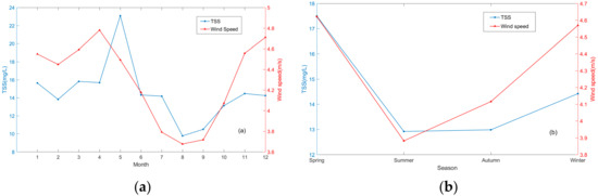
Figure 12.
Comparison of monthly and seasonal average wind speed and TSSs: (a) is monthly result and (b) is seasonal result).
To further explore the relationship between wind speed and TSSs, the correlation between the daily average TSSs and wind speed in the springs of 1984–2017 was analyzed (R2 = 0.20, n = 75). The hysteresis effect of wind speed on TSSs was also considered (R2 < 0.1, n = 75). Unfortunately, no satisfactory results were obtained.
In summary, tidal elevation, river discharge, and wind speed were major influence factors for TSSs’ variation in JZB. The construction of the Jiaozhou Bay bridge had a further impact on the variation of the TSSs as it influenced the hydrodynamic environment in the sea area surrounding the bridge [24,28]. However, the overall current field in Jiaozhou Bay changed little, and the scope of influence was limited within 1.5 km to the north and south of the bridge site [29,30]. Other uncontrollable factors, such as sediment resuspension caused by shipping and the high reflectance of the bottom at the river estuary, might also have played their parts in the variation of TSSs.
5. Conclusions
In this study, based on the field-measured TSSs and Landsat images of JZB between 1984 and 2020, a “leave-one-out cross-validation” method was used to establish a quantitative retrieval model of the JZB TSSs. Next, the temporal and spatial distribution characteristics of the JZB TSSs were analyzed, along with the main influencing factors.
This paper verifies the ability of the remote sensing algorithm to monitor TSS variations in JZB. The TSS retrieval model proposed in this paper demonstrated a satisfying performance, with R2 = 0.77 and RMSE = 1.82 mg/L. The annual average TSSs in JZB showed a downward trend as a whole, reaching their highest value in 1993 and their lowest value in 2016. Affected by the strong winds in JZB in spring and winter, the TSSs varied significantly with the seasons. The TSS concentration was high in spring and winter and low in summer and autumn. Correspondingly, the monthly average TSSs peaked in May and the lowest values appeared in August. The spatial distribution of the TSSs in JZB was similar at different timepoints, with high values appearing in the northwest of JZB and gradually decreasing to the southwest. The TSSs during the spring tide were higher than those during the neap tide, and the TSSs during the flood tide were higher than those during the ebb tide. High TSSs occurred when the tidal elevation was low, and the range of variation of the tidal elevation within a day played an important part in the range of variation of TSSs. The discharge of the Dagu River only affected the estuary and near-shore area; increased discharge brought in more sediment, although the high reflectance of the bottom caused the results to be insignificant at the river estuary. Both the wind direction and speed affected the distribution of TSSs in JZB. The wind speed had a significant effect on the seasonal variation of TSSs in JZB.
Our results showed that this empirical model based on Landsat satellite data could effectively monitor the long-term variation of TSSs in JZB. This not only provides new ideas for subsequent research but also provides a scientific basis for water quality monitoring and the rational management of JZB. In the future, the latest generation of ocean color sensors (Sentinel-2/MSI and Sentinel-3/OLCI) might provide better spatiotemporal resolutions for TSS observations in JZB.
Author Contributions
Conceptualization, J.H.; methodology, J.H., X.Z., Y.S. and J.C.; software, X.Z.; validation, J.H., X.Z.; formal analysis, J.H.; data curation, X.Z.; writing—original draft preparation, X.Z.; writing—review and editing, J.H.; visualization, X.Z.; supervision, J.H.; project administration, J.H.; funding acquisition, J.H. All authors have read and agreed to the published version of the manuscript.
Funding
This study is funded by the National Natural Science Foundation of China (Nos. 42076185 and 41706194) and SDUST Research Fund (2019TDJH103).
Conflicts of Interest
The authors declare no conflict of interest.
References
- Yang, G.; Jiang, T.; Zhao, Y.; Huang, J. Study on variation in chlorophyll-a concentration and its influencing factors of Jiaozhou Bay based on long term remote sensing images. Haiyang Xuebao 2019, 41, 183–190, (In Chinese with English Abstract). [Google Scholar]
- Yuan, Y.; Jalón-Rojas, I.; Wang, X.; Song, D. Design, construction and application of a regional ocean database: A case study in Jiaozhou Bay, China. Limnol. Oceanogr. Meth. 2019, 17, 210–222. [Google Scholar] [CrossRef]
- Zhang, Y.; Wu, Z.; Liu, M.; He, J.; Wang, M.; Yu, Z. Thermal structure and response to long-term climatic changes in Lake Qiandaohu, a deep subtropical reservoir in China. Limnol. Oceanogr. 2014, 59, 1193–1202. [Google Scholar] [CrossRef]
- Zhang, M. Distribution and seasonal variation of suspended matter in sea water of Jiaozhou Bay. Studia Mar. Sin. 2000, 2000, 49–54. (In Chinese) [Google Scholar]
- Bi, L.; Bai, J.; Zhao, Z.; Li, Y.; Yuan, Z. Characteristic of suspended particles in summer in Jiaozhou Bay. Mar. Environ. Sci. 2007, 6, 518–522, (In Chinese with English Abstract). [Google Scholar]
- Yu, S.; Mantravadi, V.S. Study on Distribution Characteristics of Suspended Sediment in Yellow River Estuary Based on Remote Sensing. J. Indian Soc. Remote Sens. 2019, 47, 1507–1513. [Google Scholar] [CrossRef]
- Zhang, M.; Tang, J.; Dong, Q.; Song, Q.; Ding, J. Retrieval of total suspended matter concentration in the Yellow and East China Seas from MODIS imagery. Remote Sens. Environ. 2009, 114, 114,392–403. [Google Scholar] [CrossRef]
- Hou, L.; Ma, A.; Hu, J.; Shan, G.; Deng, J.; Han, J.; Ding, Z. Study on remote sensing retrieval model optimization of suspended sediment concentration in Jiaozhou Bay. Period. Ocean Univ. China 2018, 48, 98–108, (In Chinese with English Abstract). [Google Scholar]
- Han, X.; Chen, X.; Feng, L. Four decades of winter wetland changes in Poyang Lake based on Landsat observations between 1973 and 2013. Remote Sens. Environ. 2015, 156, 426–437. [Google Scholar] [CrossRef]
- Benjamin, B.; Jochem, V.; Jean-Philippe, G. Assessment of Workflow Feature Selection on Forest LAI Prediction with Sentinel-2A MSI, Landsat 7 ETM+ and Landsat 8 OLI. Remote Sens. 2020, 12, 915. [Google Scholar]
- Yu, X.; Salama, M.S.; Shen, F.; Verhoef, W. Retrieval of the diffuse attenuation coefficient from GOCI images using the 2SeaColor model: A case study in the Yangtze Estuary. Remote Sens. Environ. 2016, 175, 109–119. [Google Scholar] [CrossRef] [Green Version]
- Xu, J.; Bao, J.; Yu, C.; Yang, F. Ocean Tides and Water Level Control; Wuhan University Press: Wuhan, China, 2020. (In Chinese) [Google Scholar]
- Li, M.; Kong, F.; Li, Y.; Zhang, J.; Xi, M. Ecological indication based on source, content, and structure characteristics of dissolved organic matter in surface sediment from Dagu River estuary, China. Environ. Sci. Pollut. Res. 2020, 27, 45499–45512. [Google Scholar] [CrossRef] [PubMed]
- Gao, Z.; Song, C.; Cai, Y.; Wang, M.; Feng, J.; Zhang, C. Construction and Practice of Hydrological Elements Monitoring System in Dagu River Basin; Water Resources and Hydropower Press: Beijing, China, 2017. (In Chinese) [Google Scholar]
- Feng, L.; Hu, C.; Chen, X. Influence of the Three Gorges Dam on total suspended matters in the Yangtze Estuary and its adjacent coastal waters: Observations from MODIS. Remote Sens. Environ. 2014, 140, 779–788. [Google Scholar] [CrossRef]
- Kuang, R.; Zhao, Y.; Luo, W.; Zhang, G.; Chen, Y. Study on inversion model of suspended sediment concentration based on optical classification of water body in Poyang Lake. J. China Hydrol. 2017, 37, 23–28. [Google Scholar]
- Yao, R.; Cai, L.; Liu, J.; Zhou, M. GF-1 Satellite Observations of Suspended Sediment Injection of Yellow River Estuary, China. Remote Sens. 2020, 12, 3126. [Google Scholar] [CrossRef]
- Huang, J.; Wu, M.; Cui, T.; Yang, F. Quantifying DOC and its controlling factors in major Arctic Rivers during ice-free conditions using Sentinel-2 data. Remote Sens. 2019, 11, 2904. [Google Scholar] [CrossRef] [Green Version]
- Gao, G.; Wang, X.; Bao, X.; Song, D.; Lin, X.; Qiao, L. The impacts of land reclamation on suspended-sediment dynamics in Jiaozhou Bay, Qingdao, China. Estuar. Coast. Shelf Sci. 2018, 206, 61–75. [Google Scholar] [CrossRef]
- Li, Y.; Wang, X. Tracking the multidecadal variability of the surface turbidity maximum zone in Hangzhou Bay, China. Int. J. Remote Sens. 2019, 40, 9519–9540. [Google Scholar] [CrossRef]
- He, X.; Bai, Y.; Pan, D.; Huang, N.; Dong, X.; Chen, J. Using geostationary satellite ocean color data to map the diurnal dynamics of suspended particulate matter in coastal waters. Remote Sens. Environ. 2013, 133, 225–239. [Google Scholar] [CrossRef]
- Wang, C.; Liu, Z.; Harris, C.K.; Wu, X.; Wang, H.; Bian, C.; Bi, N.; Duan, H.; Xu, J. The Impact of Winter Storms on Sediment Transport Through a Narrow Strait, Bohai, China. J. Geophys. Res. Ocean. 2020, 125, e2020JC016069. [Google Scholar] [CrossRef]
- Zhang, X.; Fichot, C.; Baracco, C.; Guo, R.; Neugebauer, S.; Bengtsson, Z.; Ganju, N.; Fagherazzi, S. Determining the drivers of suspended sediment dynamics in tidal marsh-influenced estuaries using high-resolution ocean color remote sensing. Remote Sens. Environ. 2020, 240, 111682. [Google Scholar] [CrossRef]
- Zhao, K.; Qiao, L.; Shi, J.; He, S.; Li, G.; Yin, P. Evolution of sedimentary dynamic environment in the western Jiaozhou Bay, Qingdao, China in the last 30 years. Estuar. Coast. Shelf Sci. 2015, 163, 244–253. [Google Scholar] [CrossRef]
- Ou, S.; Yang, Q.; Luo, X.; Zhu, F.; Luo, K.; Yang, H. The influence of runoff and wind on the dispersion patterns of suspended sediment in the Zhujiang(Pearl) River Estuary based on MODIS data. Acta Oceanol. Sin. 2019, 38, 26–35. [Google Scholar] [CrossRef]
- Anthony, R.; James, C.G.; Phillippe, E.T. Estuarine Suspended Sediment Dynamics: Observations Derived from over a Decade of Satellite Data. Front. Mar. Sci. 2017, 4, 233. [Google Scholar]
- Colosimo, I.; de Vet, P.L.M.; van Maren, D.S.; Reniers, A.J.H.M.; Winter, J.C.; van Prooijen, B.C. The Impact of Wind on Flow and Sediment Transport over Intertidal Flats. J. Mar. Sci. Eng. 2020, 8, 910. [Google Scholar] [CrossRef]
- Zarzuelo, C.; Lopez-Ruiz, A.; D’Alpaos, A.; Carniello, L.; Ortega-Sanchez, M. Assessing the morphodynamic response of human-altered tidal embayments. Geomorphology 2018, 320, 127–141. [Google Scholar] [CrossRef]
- Zhang, W.; Chi, W.; Hu, Z.; Liu, J.; Zhang, Y. Numerical study on the effect of the Jiaozhou Bay Bridge construction on the Hydrodynamic conditions in the surrounding sea area. Coast. Eng. 2015, 34, 40–50, (In Chinese with English Abstract). [Google Scholar]
- Yuan, Y.; Jalón-Rojas, I.; Wang, X. Impact of Coastal Infrastructure on Ocean Colour Remote Sensing: A Case Study in Jiaozhou Bay, China. Remote Sens. 2019, 11, 946. [Google Scholar] [CrossRef] [Green Version]


Publisher’s Note: MDPI stays neutral with regard to jurisdictional claims in published maps and institutional affiliations. |
© 2021 by the authors. Licensee MDPI, Basel, Switzerland. This article is an open access article distributed under the terms and conditions of the Creative Commons Attribution (CC BY) license (https://creativecommons.org/licenses/by/4.0/).